

1 Abstract
Cancers are composed of multiple genetically distinct subpopulations of cancer cells. By performing genome sequencing on tissue samples from a cancer, we can infer the existence of these subpopulations, which mutations render them genetically unique, and the evolutionary relationships between subpopulations. This can reveal critical points in disease development and inform treatment.
Here we present Pairtree, a new algorithm for constructing evolutionary trees that reveal relationships between genetically distinct cell subpopulations composing a patient’s cancer. Pairtree focuses on performing these reconstructions using dozens of cancerous tissue samples per patient, which can be taken from different points in space (e.g., primary tumour and metastasis) or in time (e.g., at diagnosis and at relapse). In concert, these can reveal thirty or more distinct subpopulations, and show how their composition changed between tissue samples.
Each additional tissue sample from a patient provides additional constraints on possible evolutionary histories, and so should aid construction of more accurate and precise results. Counterintuitively, we demonstrate using both simulated and real data that existing algorithms actually perform worse as additional tissue samples are provided, often failing to produce any result. Pairtree, conversely, efficiently leverages the information from additional samples to perform progressively better as samples are added. The algorithm’s ability to function in these settings enables new biological and clinical applications, which we demonstrate using data from 14 acute lymphoblastic leukemia cancers, with dozens of tissue samples per cancer. Pairtree also produces a useful visual representation of the degree of support underlying evolutionary relationships present in the user’s data, allowing users to make accurate inferences from its results.
2 Introduction
Individual cancers are not homogeneous entities, but are instead composed of genetically distinct cell subpopulations [1]. A cancer’s founding population typically exhibits genomic mutations acquired through time that help it overcome the controls making it cooperate as part of a larger organism [2]. As a cancer continues to grow, dividing cells inherit the mutations of their forebears while also acquiring novel mutations. Evolutionary forces such as selection and genetic drift that act on these cancer cells typically result in the emergence of genetically distinct cell subpopulations [3] (Fig. 1a).

Pairtree constructs the evolutionary tree representing the genetically distinct subclones that compose a patient’s cancer and the evolutionary relationships between them. a. A single cancer is composed of multiple genetically distinct cell subclones, represented as coloured masses. Pairtree uses one or more tissue samples taken from a patient at different points in time (e.g., diagnosis and relapse) or space (e.g., primary and metastasis). b. Each tissue sample is composed of a mixture of multiple genetically distinct cell subclones. Genomic sequencing data provides noisy estimates of each subclone’s lineage frequency in each sample—i.e., what proportion of cells in that tissue sample correspond to that subclone and its descendants. c. Pairtree uses relationships between the observed subclone lineage frequencies to infer the evolutionary tree that gave rise to the subclones, with each tree node representing a subclone. A single tree describes the complete evolutionary history of the cancer across samples. Alongside the tree, Pairtree infers the population frequency of each subclone in each tissue sample, representing the proportion of each tissue sample corresponding to that subclone. Together, the tree structure and population frequencies reveal the lineage frequencies for each subclone.

The Pairtree algorithm. Pairwise relations implied by observed lineage frequencies are compared to pairwise relations imposed by a candidate tree, with disagreement between them indicating what parts of the candidate tree are most wrong, and how that tree should be modified to improve it. Proposed tree modifications are accepted or rejected based on whether the lineage frequencies they permit are more concordant with the data than the frequencies allowed by the previous tree. The set of accepted trees collectively compose the algorithm’s posterior estimate of tree structures and lineage frequencies.
Bulk DNA sequencing data from one or more tissue samples obtained from a cancer can be used to determine the mutations that have occurred across all cell subpopulations composing the cancer. We can, in turn, use these mutations to infer the distinct cell subpopulations composing the cancer, the mutations specific to each, and the evolutionary relationships between these subpopulations [4]. A subclone is composed of a subpopulation and all descendant subpopulations that arose from it. Thus, we define a clone tree as the tree delineating the distinct cell subpopulations in a cancer, the mutations specific to each, and the proportions of cells in each sample that correspond to each subpopulation. We can computationally infer clone trees from DNA sequencing data through the process of subclonal reconstruction. Clone trees can identify important genomic mutations that occur in cancer development [3], help understand how the disease changes through time [5], and infer the selective pressures acting on the cancer [6]. Moreover, they have promising clinical applications, with the potential to predict prognosis [7, 8] and monitor how a cancer responds to treatment [9–11], with successive treatment rounds tailored to the changing composition of subpopulations [12].
Clone trees are most useful when based on multiple tissue samples taken from the same cancer, each of which is sequenced independently. Drawing on multiple tissue samples allows us to characterize more distinct cell subpopulations within the cancer, and to better infer the evolutionary relationships between them. These multiple samples may be obtained simultaneously from different spatial points in the cancer, from either the same tumour [13] or from multiple tumours (e.g., primary and metastasis) [14]. Clone trees built using these data can demonstrate how heterogeneous the cancer is within a single tumour, or how it changed between primary tumour and metastasis. Alternatively, tissue samples can be taken from the cancer at different points in time [15] (e.g., at initial diagnosis and later relapse), demonstrating, for instance, the genetic changes that drove therapy resistance to enable relapse. Cancer samples can even be used to create patient-derived xenografts or organoids that are later sequenced as distinct samples alongside the original patient samples, yielding a more detailed profile of the cancer. Using multiple patient-derived xenografts seeded from similar initial conditions, subclonal reconstructions can confer insights into the stochasticity of cancer evolution by comparing evolutionary trajectories taken by each xenograft [9].
To build clone trees, algorithms use the subclonal frequency of each observed mutation in each cancer sample, which indicates what proportion of cells carry the mutation in a given sample (fig. 1b). Algorithms estimate a mutation’s subclonal frequency based on the proportion of sequencing reads covering the mutation’s genomic locus that bear the mutation, correcting for the inferred allele-specific copy number at that locus [4]. Mutations with similar subclonal frequencies across all samples are deemed to have arisen in the same subpopulation. As each subpopulation inherits the mutations of its ancestors, increasing the subclonal frequency of those mutations, we can use the frequencies to infer evolutionary relationships between subclones and the subpopulations that compose them. The unique mutations assigned to a subpopulation are assumed to have occurred on the evolutionary path between that subpopulation and its parent. Critically, multiple tissue samples from the same cancer share a single evolutionary history, and so can be used to construct a single clone tree (Fig. 1c). The tree taken alongside the subclonal frequencies reveal the population frequencies of each subpopulation in each tissue sample, indicating what proportion of cancer cells correspond to each subpopulation.
As each cell division in cancer typically results in a parent’s progeny acquiring multiple new mutations [16], in principle a complete clone tree would render every cancer cell as an individual subpopulation. In practice, however, the limited resolution of genomic sequencing collapses many cells into each subpopulation, such that we can typically resolve between two and tens of subpopulations per cancer [1, 9]. Our ability to resolve these subpopulations is improved both by increasing sequencing depth and adding tissue samples. Both factors can help separate subpopulations that would otherwise be conflated. Greater sequencing depth imparts more precision to our estimates of subclonal frequencies, improving our ability to discern that two mutations exhibit different subclonal frequencies in at least one cancer sample, such that we can assign them to different subpopulations [17]. Likewise, increasing sequencing depth can also reveal mutations belonging to subpopulations that would otherwise lie below the detection limit of genomic sequencing. Sequencing additional tissue samples also improves subclonal reconstructions, as doing so can reveal mutations unique to the added samples that we can assign to new subpopulations. Additionally, each tissue sample grants a separate observation of each mutation’s subclonal frequency. As two mutations can be declared to belong to separate subpopulations if their subclonal frequencies differ in even one sample, additional samples thus give us the opportunity to separate subpopulations that would otherwise be merged.
Beyond resolving more subpopulations, improving data’s sequencing depth or sequencing additional samples from the same cancer also help determine the evolutionary relationships between subpopulations. Possible evolutionary relationships between subpopulations are informed by differences in their subclonal frequencies. Increasing sequencing depth improves the precision of subclonal frequency estimates, granting more certainty to our inferences about possible evolutionary relationships between subpopulations. Likewise, because each additional tissue sample grants more observations of subclonal frequencies, we can use relationships between the observed frequencies in that tissue sample and all other tissue samples to constrain possible evolutionary histories.
Clone tree reconstruction algorithms use one of two approaches: exhaustive enumeration or stochastic search. Exhaustive enumeration algorithms explicitly score all possible trees within a large pre-defined set according to how well they explain the observed data [18, 19]. With recent algorithmic advances, all trees with up to ten subpopulations can be explicitly scored in less than two hours on modern hardware [20], once mutations have been assigned to subclones. However, the number of possible trees grows exponentially with the number of subclones [21], and so this enumeration quickly becomes infeasible with more than ten subpopulations, as we demonstrate here. In general, the problem of subclonal reconstruction is NP-complete [22]. Stochastic search algorithms, conversely, use stochastic hill climbing or probabilistic sampling methods to locate high-scoring trees without requiring exhaustive enumeration [23]. Such algorithms also falter when faced with complex trees composed of many subpopulations, as we also demonstrate in this study. This may occur because the search space becomes too complex to navigate efficiently. For both enumeration and search algorithms, subclonal reconstruction should become easier with more tissue samples, since each sample confers more information about the evolutionary relationships between subpopulations. Paradoxically, we demonstrate that existing algorithms often do not benefit from adding samples, and in fact often produce progressively worse results as the number of samples increases.
Here we introduce Pairtree, a novel cancer evolutionary history reconstruction algorithm that over-comes the limitations of existing methods. Pairtree’s critical contribution is to recognize that evolutionary relationships between pairs of subpopulations can be inferred from data, and that these pairwise relationships tightly constrain the space of trees that explain the data well. With each additional tissue sample obtained from a cancer, regardless of whether the samples come from different points in space (e.g., from primary and metastasis) or in time (e.g., at diagnosis and relapse), the true pairwise relationships between subpopulations become clearer, and the correct tree becomes easier to infer. By examining subclonal frequencies of mutations, Pairtree constructs a tensor denoting the probability of each possible evolutionary relationship between subpopulations, then uses that tensor to guide a stochastic tree search. This tree search corresponds to Markov Chain Monte Carlo (MCMC) under an approximate posterior, there by allowing the algorithm to make Bayesian estimates of tree-space features, such as tree structure and subpopulation frequencies. Since Pairtree builds the pairwise relationship tensor and uses it to assist tree search, the algorithm can utilize complex datasets on which existing approaches falter—each tissue sample improves the confidence of pairwise relationship inferences, while the subsequent tree search is largely insulated from the complexity imposed by having to satisfy constraints across many samples. We demonstrate that this approach allows Pairtree to reconstruct the evolutionary history of acute lymphoblastic leukemias with up to 90 distinct subpopulations per cancer, while other algorithms often fail to produce any result.
Pairtree is available at https://www.github.com/morrislab/pairtree.
3 Methods and results
3.1 Pairtree inputs and outputs
Pairtree takes as input a set of point mutations (e.g., single-base substitutions or short indels) observed in one or more tissue samples taken from a cancer, grouping the mutations into subpopulations and constructing clone trees that describes possible evolutionary histories that gave rise to the cancer. While Pairtree can be used with only a single tissue sample, many possible solutions are often equally consistent with the data in such cases. Adding more tissue samples imposes additional constraints on evolutionary histories, such that the correct solution becomes progressively clearer.
The Pairtree algorithm uses the number of variant and reference reads observed for each mutation in each sample, with read counts originating from whole-genome sequencing (WGS), whole-exome sequencing (WES), or other sources. Pairtree uses the read counts for each mutation to compute its variant allele frequency (VAF), which is the proportion of reads spanning the mutation’s genomic locus that have the variant allele. After correcting for the effect of copy-number aberrations (CNAs), the VAF serves as a noisy estimate of each mutation’s subclonal frequency [4]. The tree search algorithm assumes that mutations have been clustered into subpopulations, such that each cluster’s mutations originated from the same subpopulation. Pairtree provides two MCMC-based algorithms for clustering mutations based on their observed subclonal frequencies, with one using the relationship tensor denoting pairwise relationships between mutations, and the other working directly from the observed mutation subclonal frequencies. Other clustering algorithms can also be used [17, 24, 25].
Pairtree produces as output a set of clone trees for a single cancer, each of which is scored by a likelihood representing how well it fits the observed data. Each tree node represents a genetically distinct cell subpopulation, associated with which is a cluster of one or more genomic mutations rendering the subpopulation genetically distinct from every other. Other mutations may exist within the cancer—subclonal reconstructions reflect only mutations whose prevalence was sufficiently high for genomic sequencing to distinguish from background noise. Together, a subpopulation and all its descendants compose an evolutionary clade, referred to as a subclone.
Edges in a clone tree reflect evolutionary descent, with an edge from node A to node B indicating that subpopulation B evolved from A. All mutations assigned to B occurred on the evolutionary path from A to B, with all of B’s descendants inheriting them. In addition, each subclone is assigned a tree-constrained subclonal frequency in each tissue sample, indicating what proportion of cells correspond to the subclone. Together, the subclonal frequencies and tree structure yield the population frequencies, indicating what proportion of cells in a cancer sample originated from a specific subpopulation.
Every clone tree has a root node corresponding to the non-cancerous population that gave rise to the cancer. By definition, this root is assigned no mutations, and has a cellular frequency of 100% in every sample. Usually, there will be only a single primary cancerous population descending from this root, representing the founding cancer cell population that gave rise to all subpopulations. However, when supported by the data, Pairtree permits poly-primary cancers composed of multiple independent cancers from the same patient.
Alternatively, Pairtree may be run on the mutations directly without first clustering them into sub-clones, yielding a mutation tree instead of a clone tree. A mutation tree is equivalent to a clone tree in which each clone bears only a single distinct mutation, such that every tree node corresponds to a unique mutation.
3.2 Computing pairwise mutation relationships
All mutations associated with a subpopulation are assumed to share the subpopulation’s subclonal frequency, representing the proportion of cells that originated from that subpopulation or its descendants. Equivalently, a subpopulation’s subclonal frequency indicates what proportion of cells carry the population’s associated mutations in a given tissue sample. By the infinite sites assumption (ISA), we assume that each genomic site is mutated at most once through the cancer’s history, meaning that descendant subpopulations inherit all their ancestors’ mutations. While violations of the ISA are possible [26], they have sufficiently little effect on evolutionary history reconstruction that methods can produce accurate results even when they occur [27]. ISA violations can in some situations be detected, as we describe subsequently. Under the ISA, a subclone’s frequency cannot be greater than its parent’s. By exploiting this constraint across all observed tissue samples, we can infer evolutionary relationships between all pairs of subpopulations. Given the ISA, four possible evolutionary relationships exist between two mutations A and B.
A and B are co-occurring. That is, A and B occur in precisely the same cell subpopulations, such that A is never present without B and vice versa. This reflects that A and B occurred proximal to each other in evolutionary time, such that we cannot distinguish an intermediate subpopulation that occurred between them.
A is ancestral to B. That is, A occurred in a population ancestral to B, such that some cells possess A without B, but no cell has B without A. This reflects that A preceded B.
B is ancestral to A, mirroring relationship 2, reflecting B preceded A.
A and B occurred on different branches of the clone tree, such that they never occur in the same set of cells. This relationship confers no information about the respective timing of A and B.
For each mutation pair, Pairtree compares the VAFs of the two mutations across every tissue sample to compute a probability distribution over these relationships for that pair. Occasionally, different samples provide strong support for conflicting relationship types, often reflecting failures of the four-gamete test [28] that stem from violations of the ISA. To account for these cases, we add a fifth possible relation, termed the garbage relation. Beyond ISA violations, high garbage probability for a mutation pair may result from technical noise that corrupts the VAF observations, or unreported CNAs that skew the relationship between VAF and cellular frequency.
In addition to mutation read counts, Pairtree takes as input mutation clusters, with each cluster representing a genetically distinct subpopulation. As all mutations within a subpopulation share the same evolutionary relationships to all other subpopulations’ mutations, we can consider pairwise relations solely between clusters rather than between individual mutations, reducing the algorithm’s computational burden. Using the mutation read counts and clusters, we thus compute a probability distribution over pairwise relations for every pair of subpopulations, yielding a data structure termed the “pairs tensor.”
3.3 Searching for trees using pairwise relations
Pairtree samples from the posterior distribution over clone trees using the Metropolis-Hastings MCMC algorithm [29]. The likelihood is defined by how well a tree’s subclonal frequencies fit the observed mutation read counts under a binomial observation model, using separate subclonal frequencies for each tissue sample. Subclonal frequencies are constrained by their tree—the root subpopulation, corresponding to the normal tissue with no mutations that gave rise to the cancer, must have a subclonal frequency of 1 in every sample. Furthermore, every subpopulation must have a frequency at least as great as the summed frequencies of its children. These subclonal frequencies are computed using one of two schemes, yielding an approximation of the maximum likelihood estimate (MLE) of tree-constrained subclonal frequencies, which in turn produces a Laplace approximation of the tree’s marginal likelihood.
New proposal trees for Metropolis-Hastings are generated using the pairs tensor, which helps in two ways. Firstly, by comparing the pairwise relations imposed by the existing tree to those implied by the data, we can identify which subclones within the tree should be modified because they are least consistent with the data. Secondly, after identifying high-error subclones, the pair tensor informs where those subclones should be moved within the tree to reduce error. While other algorithms also modify trees by moving subclones within them, they blindly choose both the subclone to move and its destination [30, 31]. Pairtree, conversely, uses its pairs tensor as a guide to rapidly move through tree space toward high-likelihood trees.
Using only pairwise relations to propose new trees can lead to the algorithm becoming stuck in local minima. These minima arise because pairwise relations do not capture higher-order relationships between three or more subpopulations. Consequently, the tree-proposal algorithm may repeatedly propose tree modifications that improve consistency with pairwise relationships while worsening the overall tree, leading to many successive proposals being rejected. To escape such minima, the algorithm stochastically proposes random tree modifications that ignore the pairs tensor. Additionally, Pairtree runs multiple independent MCMC chains in parallel, each of which uses different initial trees and takes different paths through tree space, further reducing the chance of becoming trapped in local minima.
3.4 Choosing methods to compare against Pairtree
We elected to compare Pairtree, a stochastic search method, against three exhaustive enumeration methods (PASTRI [21], CITUP [19], and LICHeE [18]) and one stochastic search method (PhyloWGS [32]).
PASTRI [21] attempts to make tree enumeration feasible by using mutation VAFs as noisy estimates of the true subclonal frequencies. The algorithm samples subclonal frequencies for every subpopulation in every tissue sample from an approximate posterior informed by mutation VAFs, then enumerates all trees consistent with the sampled frequencies. This approach falters when the VAF-informed proposal distribution for the subclonal frequencies is a poor approximation to the true posterior, as the method may never recover a set of subclonal frequencies whose consistent phylogenies include the true tree.
CITUP [19] enumerates all trees possessing a given range of subpopulations. For each possible tree topology, CITUP attempts to determine the optimal assignment of subpopulations to tree nodes that permits subclonal frequencies matching the mutation data as well as possible. As this enumeration is unconstrained, CITUP can struggle to deal with many subpopulations, which presumably permit too many possible tree topologies.
LICHeE [18] uses mutation VAFs to construct a graph containing possible parent-child relationships between subpopulations, then enumerates all spanning trees of this graph that obey tree constraints. Thus, its tree enumeration need not consider nearly as many trees as CITUP, allowing it to scale better.
PhyloWGS [32] uses MCMC to search for trees, sampling trees with Metropolis-Hastings and fitting subclonal frequencies to each tree. As a search-based algorithm, PhyloWGS scales more easily to many-subpopulation trees than most enumeration-based methods.
3.5 Metrics for evaluating methods
To compare subclonal reconstruction algorithms, we developed two metrics. While past method comparisons have developed metrics for evaluating methods [33], we required new measures that are well-suited to the multi-sample domain.
The first, termed VAF reconstruction loss (henceforth “VAF loss”), measures how well a tree’s subclonal frequencies match the cellular frequency for each mutation implied by its VAF. Each tree structure permits a range of subclonal frequencies, with the best subclonal frequencies matching the data as well as possible while also satisfying the tree constraints. Thus, the VAF loss evaluates a tree by determining how closely its subclonal frequencies match the observed data. VAF loss is reported in in bits per mutation per tissue sample, representing the number of bits required to describe the data using the tree, normalized to the number of mutations and tissue samples. Lower values reflect better trees. As LICHeE could not compute subclonal frequencies itself, producing only tree structures, we used Pairtree to compute the MLE subclonal frequencies for its trees.
All evaluated methods report multiple solutions for each dataset, scored by a method-specific likelihood or error measure. To determine a single VAF loss for each method on each dataset, we used the method-specific solution scores to compute the expectation over VAF loss (equivalent to the weighted-mean VAF loss). VAF loss is always reported relative to a baseline. For simulated data, the baseline is the VAF loss achieved using the true subclonal frequencies that generated the data. For real data, the baseline is expert-constructed, manually-built trees that were subjected to extensive refinement, with Pairtree used to compute the MLE subclonal frequencies. Thus, VAF loss indicates the average extra number of bits necessary to describe the data using a method’s solutions rather than the baseline solution. Methods can find solutions that fit the data better than the baseline, yielding a negative VAF loss.
The second evaluation metric we developed, termed relationship reconstruction error (henceforth “relationship error”), recognizes that a clone tree defines pairwise relations between its constituent mutations, placing every pair in one of the four relationships discussed earlier. Using the set of trees reported by a method for a given dataset, we computed the empirical categorical distributions over pairwise mutation relations, with each tree’s relationships weighted by the likelihood or error measure reported by the method. We then compared these distributions to the distributions imposed by all tree structures permitted by the true subclonal frequencies, computing the Jensen-Shannon divergence (JSD) between distributions for each pair. This yields a relationship error ranging between 0 bits and 1 bit. Using these, we report the joint JSD across all mutation pairs to summarize the quality of the solution set, normalized to the number of pairs. Thus, the relationship error for a given dataset ranges between 0 bits and 1 bit, with smaller values indicating that a method better recovered the full set of trees consistent with the data. We did not use this metric with real data, whose true subclonal frequencies, and thus true possible tree structures, are unknowable.
3.6 Existing algorithms often fail on simulated data
We validated algorithm performance on 576 simulated datasets across a range of parameters. These included trees with three, ten, 30, or 100 subpopulations. Three subpopulations are often the maximum one can resolve using single tissue samples with thousands of mutations at typical WGS read depths of 50x [1]. Ten subpopulations are possible when given multiple tissue samples [34], while thirty were the approximate maximum we could resolve in the high-depth, many-sample acute lymphoblastic leukemia data that motivated Pairtree’s creation. We also included datasets with 100 subpopulations to push the algorithms’ limits. The number of simulated tissue samples ranged from one to 100, while we also varied the numbers of mutations per population and read depth per mutation. For the 30- and 100-subpopulation settings, we did not include one- or three-sample datasets, as resolving so many subpopulations from so few samples would be unrealistic.
We generated each dataset through a three-step process: we sampled the tree structure, then sampled subclonal frequencies for each tree subpopulation in each tissue sample, then assigned mutations to the subpopulations and sampled their read counts based on their subpopulation’s frequencies. Each subclonal reconstruction method was given the true mutation clusters, allowing us to evaluate how well methods can construct trees after mutations have already been grouped into subpopulations. CITUP and LICHeE can cluster mutations themselves or can take pre-computed clusters as input, while Pairtree and PASTRI require pre-computed clusters. PhyloWGS insists on clustering mutations itself, which complicated method comparisons. All methods were allowed up to 24 hours of compute time, but often crashed or failed to produce a result within this period.
All comparisons algorithms struggled to deal with simulated data possessing many tissue samples, many subpopulations, or both (Fig. 3a). CITUP failed to produce results on any dataset with ten or more subpopulations. PASTRI could not produce a tree for 83% of three-subpopulation datasets and 96% of ten-subpopulation datasets, and does not support running with more than fifteen subpopulations [35]. LICHeE and PhyloWGS fared better, with both algorithms producing results on all three-, ten-, and thirty-subpopulation simulations. LICHeE failed, however, on 92% of 100-subpopulation datasets, while PhyloWGS failed on 38% of them. Pairtree successfully produced results on all 108 datasets with 100 subpopulations.

Algorithm success rates, lineage frequency errors, and pairwise relation errors on 576 simulated datasets. Mid-lines in box plots indicate medians. a. Comparison algorithms often either crashed or failed to finish within 24 hours. Only Pairtree ran successfully on all 576 datasets. For datasets with ten or more subclones, CITUP and PASTRI failed on all but a small minority. LICHeE and PhyloWGS ran successfully on all datasets with 30 or fewer subclones, failing only in the 100-subclone setting. b. Lineage frequency error indicates how discordant the lineage frequencies computed by an algorithm are relative to the true frequencies used to generate the data, with high error reflecting poor-quality trees. Each method’s result includes only datasets on which it ran successfully. Error is reported for each dataset in terms of negative log likelihood, normalized to the number of mutations and tissue samples in the dataset. For trees with 30 or fewer subclones, Pairtree often exhibits negative error, indicating it found the true tree structure or equally good candidates. Other methods generally exhibit progressively higher error as the number of subclones increases. c. Pairwise relation error represents the average error in pairwise relations implied by the tree structures reported by each method, relative to the pairwise relations implied by the range of tree structures consistent with the true lineage frequencies. Each score indicates the Jensen-Shannon divergence between the true distributions over pairwise relations and proposed distributions normalized to the number of pairs, such that errors necessarily range between zero bits and one bit. As with lineage frequency error, Pairtree exhibits lower error than comparison methods until the 100-subclone setting. The pairs tensor Pairtree uses to generate proposed trees exhibits lower average error than other methods, and only slightly higher error than the full Pairtree algorithm, while using only a fraction of the computation.
3.7 Pairtree exhibits lower error than other algorithms on simulated data with thirty or fewer subpopulations
As Pairtree was the sole method that produced results for all 576 simulations, its results reflect its performance on all datasets, while results for other methods reflect their performance on only the subset for which they succeeded.
Pairtree fared better than any comparison algorithm on trees with three, ten, or thirty subpopulations, succeeding on all datasets while achieving negative median VAF losses in all three settings (Fig. 3b). Pairtree also performed better than the comparison algorithms with respect to relationship error (Fig. 3c). In general, for these settings, relationship error was almost zero when the number of tissue samples exceeded the number of subpopulations. For such cases, only one possible tree occurred, with Pairtree finding that tree (or a close approximation thereof) and placing high confidence in it. The pairs tensor that Pairtree computes as a guide for tree search also delineates pairwise relationships accurately (Fig. 3c), requiring only a fraction of the computational resources of the full Pairtree algorithm. Though it does slightly worse than full Pairtree, as it cannot exploit information about higher-order relationships that become apparent during tree search, it nevertheless achieves less relationship error than any algorithm except full Pairtree.
LICHeE was the next-best performing algorithm, also succeeding on all datasets with three, ten, or thirty subpopulations and achieving low VAF losses in these settings (Fig. 3b). With respect to relationship errors, LICHeE performed moderately well (Fig. 3c), except for cases with thirty subpopulations.
PASTRI performed well when it produced a result, reaching negative median VAF losses for three and ten subpopulations, and relatively low relationship errors (Fig. 3b and Fig. 3c). However, these reflect its performance on only the 17% of three-subpopulation and 4% of ten-subpopulation cases where it succeeded. Additionally, PASTRI occasionally produced poor results, with a maximum lineage frequency error of 492 bits on one three-subpopulation dataset.
CITUP produced mediocre results for three-subpopulation cases, suffering high VAF losses (Fig. 3b). However, its relationship errors were lower than for other comparison methods (Fig. 3c), suggesting that the tree structures it recovered were reasonably accurate, even if it struggled to fit good subclonal frequencies to these structures. Notably, CITUP produced results for only 68% of these datasets (Fig. 3a), while failing on all ten-, thirty-, and 100-subpopulation cases.
PhyloWGS succeeded on all datasets with thirty subpopulations or fewer (Fig. 3a), but achieved worse VAF losses than Pairtree and LICHeE (Fig. 3b). These comparisons, however, were biased against PhyloWGS, which was the sole method that could not take a pre-computed mutation clustering as input. We provided as much clustering information to PhyloWGS as possible, preventing the method from splitting clusters such that mutations from the same cluster would be assigned to different subpopulations. Nevertheless, PhyloWGS could still merge clusters such that multiple clusters’ variants would be assigned to the same subpopulation. This behaviour was responsible for most of PhyloWGS’ poor results.
Given that non-Pairtree methods may have been particularly prone to failing on the most challenging simulations, summary statistics reported for these methods may be unfairly biased in their favour, as they would only reflect performance on less-challenging datasets. Nevertheless, when we compare Pairtree to each method on only the subset of datasets for which the comparison method succeeded (Fig. 4), we see that Pairtree almost always produces better VAF losses, with the only exception being several 100-subpopulation datasets where PhyloWGS beat Pairtree.

Lineage frequency error of each algorithm relative to Pairtree. Each point represents a method’s lineage frequency error on a simulated dataset relative to Pairtree, with positive values indicating worse error. As each method failed on different simulations (Fig. 3a), values are reported only on datasets where a method produced a result. Across the 576 simulations, Pairtree always produced lower error than every other method, excepting 15% of the 100-subclone datasets (16 of 108) where PhyloWGS performed better.
3.8 All algorithms struggle on 100-subpopulation cases
None of the algorthms performed well on 100-subpopulation datasets, illustrating the difficulty of phylogeny construction at this scale. Pairtree produced results for all 108 datasets with 100 subpopulations, but exhibited higher VAF losses than on smaller trees (Fig. 3b). Likewise, its relationship errors on 100-subpopulation trees were also worse. The pairs tensor was better able to delineate pairwise relationships between mutations than the full Pairtree algorithm, serving as a marked contrast to settings with fewer subpopulations where the full Pairtree algorithm did better. This illustrates the challenges of navigating tree space for such large trees.
Both PhyloWGS and LICHeE also struggled with 100-subpopulation trees. PhyloWGS failed on 14% of simulations with 30 samples and all of the 100-sample instances. LICHeE exhibited similar behaviour, failing on 75% of 10-sample cases, and all 30- and 100-sample cases. On the different simulation subsets where they succeeded, both algorithms demonstrated VAF losses on par with Pairtree.
3.9 Both error and failure rate increase for other algorithms as the number of tissue samples increases
Non-Pairtree methods struggled to deal many simulated tissue samples. The failure rate of the two worse-performing comparison methods, CITUP and PASTRI, increased with the number of tissue samples for both three- and ten-subpopulation trees (Fig. 5a). Similarly, the two better-performing methods, LICHeE and PhyloWGS, exhibited increasing VAF losses as the number of samples increased (Fig. 5b). Pairtree, by contrast, exhibited no failures and effectively zero median VAF loss regardless of the number of simulated tissue samples. With respect to relationship errors, the performance of both full Pairtree and the pairs tensor improved with more samples (Fig. 5c). LICHeE, conversely, exhibited rapidly increasing error with more samples, while PhyloWGS’ performance fluctuated.

Examining algorithm performance in greater depth suggests why comparison algorithms faltered. a. Success rate varied according to the number of subclones and number of tissue samples for the two worst-performing comparison algorithms, CITUP and PASTRI. They failed on an increasing proportion of datasets as the number of simulated tissue samples increased in both the three- and ten-subclone settings. Pairtree succeeded on all such datasets. b. Median lineage frequency error varied according to the number of subclones and tissue samples for the two better-performing comparison algorithms, LICHeE and PhyloWGS. Error bars represent the first and third quartiles. All three algorithms succeeded on all datasets in these settings. LICHeE and PhyloWGS, however, generally exhibited higher error as the number of tissue samples increased, while Pairtree’s error remained near-zero across these settings. c. As with lineage frequency error, median pairwise relation error varied according to the number of subclones and tissue samples. In general, LICHeE suffered higher error as the number of tissue samples increased, while PhyloWGS, Pairtree, and the pairs tensor Pairtree uses for tree search achieved lower error with more tissue samples.
As each tissue sample provides additional information about evolutionary relationships between sub-populations, subclonal reconstruction should become easier with more samples. Pairtree takes advantage of this, exploiting the information provided by additional samples to more accurately infer pairwise evolutionary relationships and produce more accurate reconstructions. Other algorithms, however, did not manage this, instead performing worse as the number of samples increased. In general, this may be because they struggled to satisfy the full set of tree constraints across many samples.
3.10 Pairtree exhibits lower error than other algorithms on 14 acute lymphoblastic leukemias
We applied Pairtree to genomic data from 14 acute lymphoblastic leukemia patients [9]. There were 16 to 509 mutations called per patient (median 40), clustered into 5 to 26 subpopulations per patient (median 8), across 13 to 90 tissue samples per patient (median 42). Tissue samples included one or more samples taken at diagnosis and at relapse from each patient and subjected to WES. Each sample was then used to seed multiple patient-derived xenografts (PDXs) in mice, which were later subjected to targeted sequencing with target loci determined by what variants were discovered in the patient WES samples. The median read depth across cancers was 212 reads, while the mean was 220 reads.
We applied Pairtree, CITUP, LICHeE, PASTRI, and PhyloWGS to these data. CITUP and PASTRI failed on 13 of the 14 cancers, and so we excluded them from the comparison. In comparing the algorithms’ performance using VAF loss, our baseline could not be the true subclonal frequencies, like in the simulated data, as the true frequencies are unknowable. Instead, we built high-quality clone trees for each dataset manually, subjecting them to extensive review and refinement. We then fit MLE subclonal frequencies to these using Pairtree, yielding the expert-derived baseline. As in simulation, methods could improve upon this baseline to yield negative error.
Pairtree found effectively equivalent trees to the baseline for 12 of 14 cancers (Fig. 6), resulting in VAF losses between 0 and −0.05 bits. On two cancers, Pairtree found better-than-baseline trees, resulting in losses of −0.32 bits and −1.42 bits. LICHeE beat the baseline for one cancer, reaching a loss of −0.86 bits; matched the baseline for four other patients, incurring between 0 and 0.11 bits of loss; and had substantially worse losses for the remaining nine patients. PhyloWGS suffered at least 0.35 bits of loss on all patients, reaching a median VAF loss of 4.42 bits. As in simulated data, PhyloWGS’ performance was impaired by its inability to strictly adhere to the provided clustering, causing it to frequently merge clusters.

Lineage frequency error for 14 acute lymyphoblastic leukemia datasets, with 13 to 90 tissue samples per patient. Mid-lines in box plots indicate medians. CITUP and PASTRI each failed on 13 of 14 datasets and so are not shown. Lineage frequency errors are reported as a negative log likelihood normalized to the number of mutations and tissue samples, relative to the likelihhood realized by the lineage frequencies permitted by manually constructed trees built by experts. Across all 14 cancers, Pairtree matched or improved upon the lineage frequency errors achieved in the manually constructed baseline, which no other method managed.
Relationship errors are not considered for this dataset, as computing them requires knowing the set of trees consistent with the (unknowable) true subclonal frequencies.
3.11 Pairtree can intuitively illustrate uncertainty in cancer phylogenies
Pairtree creates visualizations that make explicit how uncertain its results are. All trees the algorithm sampled for a dataset are combined into a single graph whose edges are weighted by the trees’ posterior probabilities, yielding a visualization termed the consensus graph. This is critical for interpreting Pairtree’s results, as users typically want a single tree representing the evolutionary history of their dataset. When methods report multiple possible solutions, as do all methods considered here, users will often select the single tree with the highest likelihood or score. This single solution, however, will not reflect other credible tree candidates that support the user’s data nearly as well as the highest-scoring one, potentially leading to incorrect inferences about tree features. Moreover, that single solution typically presents all evolutionary relationships between subpopulations as equally certain. Pairtree’s consensus graph, conversely, characterizes the uncertainty present in its results, representing all credible possibilities and the uncertainty underlying each. This allows users to make informed conclusions about biological and clinical questions.
For instance, given a 17-subpopulation tree we built for one of the fourteen acute lymphoblastic leukemias on which we ran Pairtree (Fig. 7), a tree built with only a single tissue sample will, in isolation, appear no less certain than a tree built using all 90 available tissue samples. However, by examining the consensus graph representing all plausible trees for the data, the user will see that there’s enormous uncertainty in the single-sample trees, which is all but eliminated when using dozens of samples. For instance, Pairtree is confident that population 17’s parent is population 13, but most other populations have many possible parents, such that the subpopulation with the least-certain placement can resolve its parent with only 7% certainty. As Pairtree is provided with more samples, it can resolve evolutionary relationships with greater certainty. With 30 samples, most evolutionary relationships become clear, and all relationships are resolved with at least 45% certainty. Providing yet more samples increases certainty, with 90 samples allowing all parent-child relationships to be determined with at least 91% certainty, and can correct erroneous inferences—for example, with 30 samples, population 8 appeared to be the likely parent of population 15, but with 90 samples, it became clear that population 15’s parent is population 6.

Pairtree can visualize the uncertainty in its posterior tree distribution, helping the user understand how certain each evolutionary relationship is. Depicted here are consensus graph visualizations for one of the 14 acute lymphoblastic lekuemia patients analyzed with Pairtree, using a variable number of tissue samples ranging from a single sample to all 90 samples available for the patient. With only a single tissue sample, most relationships are uncertain. Once Pairtree is given 30 samples, most relationships can be resolved with certainty, with the tree becoming more certain yet when given 90 samples. All edges with 5% or greater posterior certainty are shown. The minimum spanning tree certainty indicates, if the graph is fully connected such that every population has at least one possible parent, how certain the least-certain single parent is.
4 Discussion
Before developing Pairtree, we attempted to build phylogenies for the ALL patients presented here using existing algorithms. As we had dozens of tissue samples per patient, we could resolve dozens of cancer cell subpopulations for each. All existing subclonal reconstruction algorithms failed to build clone trees for these subpopulations, presumably because most existing algorithms were not designed for settings with so many subpopulations.
When building trees with few subpopulations, exhaustive enumeration algorithms are attractive, as they promise to find the single best tree by considering all possibilities. As our simulations demonstrated, however, enumeration algorithms cannot cope with more than ten subpopulations, as the number of possible trees becomes too great, even when constraints are employed to reduce possible tree configurations. Stochastic search algorithms are a superior approach when faced with numerous subpopulations, provided they can locate high-likelihood regions of tree space and limit their search to those areas. When this space is searched blindly, however, it remains difficult to navigate, given the massive number of possible clone trees formed from having many subpopulations.
Pairtree is the first algorithms designed to work with tens of subpopulations and tens of tissue samples. The algorithm’s key advance is to recognize that evolutionary relationships between pairs of subpopulations can be inferred from data, and these serve as an effective guide to navigating tree space. By computing probability distributions over pairwise relations before tree search begins, Pairee ensures that, unlike other algorithms, the difficulty of this search does not increase with more tissue samples that impose further solution constraints that must be satisfied. Crucially, more samples provide more precise information about what the correct evolutionary relationships are between subpopulations, allowing Pairtree to find better trees. Thus, Pairtree can leverage the rich constraints imposed by many tissue samples to efficiently navigate tree space, yielding accurate phylogenies even when given dozens of subpopulations. By combining these advances with consensus graph visualizations that concisely illustrate the degree of certainty present in each tree feature it produces, Pairtree can imbue cancer evolutionary history reconstructions with the accuracy and robustness necessary for novel research and clinical applications.
6 Online Methods
6.1 Computing pairwise relations
6.1.1 Establishing a probabilistic likelihood for pairwise relations
Let A and B represent two distinct mutations. We denote their observed read counts, encompassing both variant and reference reads, as xA and xB. Assuming both mutations obey the ISA, the pair (A, B) must fall in one of four pairwise relationships, denoted by MAB.
MAB = coincident, meaning A and B are co-occurring. That is, A and B occur in precisely the same cell subpopulations, such that A is never present without B and vice versa. This reflects that A and B occurred proximal to each other in evolutionary time, such that we cannot distinguish an intermediate subpopulation that occurred between them.
MAB = ancestor, meaning A is ancestral to B. That is, A occurred in a population ancestral to B, such that some cells possess A without B, but no cell has B without A. This reflects that A preceded B.
MAB = descendent, meaning B is ancestral to A. This mirrors relationship 2, reflecting B preceded A.
MAB = branched, meaning A and B occurred on different branches of the clone tree, such that they never occur in the same set of cells. This relationship confers no information about the respective timing of A and B.
To the four possible relationships above, we add a fifth, termed the garbage relation and denoted by MAB = garbage. This represents mutation pairs with conflicting evidence for different relationships amongst the four already defined, providing a baseline against which the other four relationships can be compared.
The likelihood of the pair’s relationship is written as p(xA, xB|MAB). First, we note that every tissue sample s can be considered independently of others, allowing us to factor the likelihood.

To compute the pairwise relationship likelihood for one tissue sample s, we integrate over the possible subclonal frequencies associated with the subclones that gave rise to mutations A and B, representing the proportions of cells in the tissue sample carrying the mutations. We indicate these subclonal frequencies as ϕAs and ϕBs.

As each mutation’s likelihood is a function solely of its subclonal frequency, and is independent of both the other mutation and the pairwise relationship, we can simplify the integral.

6.1.2 Defining a binomial observation model for read count data
We can now begin providing concrete definitions for each factor in the integral given in Eq. (1). For mutation j ∈ {A, B} from tissue sample s, whose observed read count data are represented by xjs, we define p(xjs|ϕjs) using the following notation:
ϕjs: subclonal frequency of subclone where j originated
Vjs: number of genomic reads of the j locus where the variant allele was observed
Rjs: number of genomic reads of the j locus where the reference allele was observed
ωjs: probability of observing the variant allele in a subclone containing j. Equivalently, this can be thought of as the probability of observing the variant allele in a cell bearing the j mutation. Thus, in a diploid cell,
 .
.

Observe that ωjs can be used to indicate changes in ploidy. For instance, a variant lying on either of the sex chromosomes in human males would have ωjs = 1, since males possess only one copy of the X and Y chromosomes, so no wildtype allele would be present. Alternatively, ωjs can indicate clonal copy number changes, such that all cancer samples in a sample bore the same CNA. If, for instance, the founding cancerous subclone bearing a mutation underwent a duplication of the wildtype allele, then, once the mutation arose in a descendent subclone, every cell within that subclone would contribute two wildtype alleles and one variant allele. Thus, in this instance, we would have  . While this representation requires that the CNA be clonal, any SNVs affected by the CNA can be subclonal, and can in fact belong to different subclones.
Though this scheme can represent clonal CNAs, it cannot do so for subclonal CNAs. Fundamentally, the tree-building algorithm requires converting the observed  values into estimates of subclonal frequencies
  . If a subclonal CNA overlapping the mutation j occurs, different subclones will contribute different numbers of alleles to the tissue sample, implying this relationship is no longer valid. While the model could be extended to place subclonal CNA events on the clone tree and estimate how they change
  , our experience in the Pan-Cancer Analysis of Whole Genomes project suggested widespread disagreement between subclonal CNA-calling algorithms [1], such that we could construct accurate clone trees only by discarding variants in subclonally CN-aberrated regions.
Using this notation, let the likelihood of observing Vjs variant reads for mutation j in sample s, given a subclonal frequency ϕjs, be defined by the binomial. We have Vjs + Rjs observations of j’s genomic locus, and probability ωjsϕjs of observing a variant read, representing the proportion of alleles in the sample carrying the variant.

6.1.3 Defining constraints on subclonal frequencies imposed by pairwise relationships
To be fully realized, the likelihood Eq. (1) now requires only p(ϕAs, ϕBs|MAB) to be defined. We use this factor to represent whether ϕAs and ϕBs are consistent with the relationship MAB. For the ancestor, descendent, and branched relationships, the subclonal frequencies ϕAs and ϕBs dictate whether a relationship is possible.

The subclonal frequencies ϕAs and ϕBs may each take values on the [0,1] interval. Thus, p(ϕAs, ϕBs|MAB) for MAB ∈ {ancestor, descendent, branched} are each non-zero only inside a right triangle lying within the unit square on the Cartesian plane with corners at (ϕAs, ϕBs) ∈ {(0, 0), (0, 1), (1, 0), (1, 1)}. The location of the triangle within the unit square differs for each of the three MAB relationships, but all have an area of  . Consequently, to ensure ∬dϕAsdϕBsp(ϕAs, ϕBs|MAB) = 1, we set
  . Thus, p(ϕAs, ϕBs|MAB) = C = 2 when ϕAs and ϕBs are consistent with MAB, and zero otherwise.
We must still define the remaining two relationships MAB ∈ {coincident, garbage}. The garbage relationship permits all combinations of ϕAs and ϕBs lying within the unit square, such that p(ϕAs, ϕBs|MAB = garbage) = 1. Consequently, unlike the previous three relationships, the garbage relationship imposes no constraints on ϕAs and ϕBs relative to each other.

The garbage relationship serves to establish a baseline against which evidence for the non-garbage relationships can be evaluated. Observe that, in Eq. (1), p(xAs|ϕAs)p(xBs|ϕBs) is integrated over the unit square when MAB = garbage. Conversely, when MAB ∈ {ancestor, descendent, branched}, we integrate p(xAs|ϕAs)p(xBs|ϕBs) over a triangle covering half the square. Consequently, 
 . This arises because p(ϕAs, ϕBs|MAB) = 2 for subclonal frequencies consistent with MAB ∈ {ancestor, descendent, branched}, while p(ϕAs, ϕBs|MAB) = 1 for subclonal frequencies consistent with MAB = garbage. When the read counts for the mutations A and B clearly permit one of the three non-garbage relationships, most of the probability mass of the two associated binomials will reside within the simplex permitted by the relationship, and so the evidence for the non-garbage relationship will be nearly double that of the evidence for garbage. Conversely, when the read counts push most of the binomial mass outside the permitted simplex, the non-garbage evidence will be substantially lower than the baseline provided by garbage.
By considering accumulated evidence across many tissue samples, the garbage model’s utility becomes clear. If, across many tissue samples for a mutation pair, the evidence for one non-garbage relationship is consistently favoured over others, then that relationship will emerge as the most likely when the evidence is considered collectively across samples. However, if different tissue samples favour different relationship types, the steady accumulation of the baseline garbage evidence could, in concert, be more than the evidence for any of the other three relations, meaning garbage would be declared as the most likely relationship for the mutation pair. Mutations that make up many pairs with high garbage evidence are best excluded from clone tree construction, as such mutations likely suffered from uncalled CNAs, violations of the ISA, or erroneous read count data.
The only undefined relationship remaining is MAB = coincident. As the coincident relationship dictates that two mutations arose from the same subclone, and so share the same subclonal frequency, the corresponding constraint is defined thusly:

6.1.4 Efficiently computing evidence for ancestral, descendent, and branched pairwise relationships
We now consider how to compute the pairwise likelihood given in Eq. (1) for MAB ∈ {ancestor, descendent, branched}.

Observe that we can rearrange the integral to move the factor corresponding to the mutation A observations outside the inner integral.

Now, because p(ϕAs, ϕBs|MAB) is piecewise-constant when MAB ∈ {ancestor, descendent, branched}, we can, for these relationships, impose this factor’s effect by changing the integration limits. Let L(ϕAs, MAB) and U(ϕAs, MAB)) represent functions whose outputs are the lower and upper integration limits, respectively, for the inner integral whose differential is dϕBs, as a function of ϕAs and the relationship MAB. These functions are defined thusly:

By writing the inner integral using these integration limits, and limiting the outer integral to the [0, 1] interval permitted for ϕAs, the factor p(ϕAs, ϕBs|MAB) can be replaced by 2, as it is constant over the interval of integration.

To render the inner integral more computationally convenient, rather than integrate over ϕBs, we would prefer to integrate over qBs ≡ ωBsϕBs. Thus, we will integrate by substitution, using  .
.

Observe that the inner integral is now simply integrating the binomial PMF over its parameter qBs. To compute this integral, we rely on the following equivalence between this integral and the incomplete beta function β:

Now we can compute the integral over an arbitrary limit by the fundamental theorem of calculus.

Finally, we combine the above results, allowing us to compute the pairwise relationship likelihood when MAB ∈ {ancestor, descendent, branched} as a one-dimensional integral.

To compute this, we use the one-dimensional quadrature algorithm from scipy.integrate.quad.
6.1.5 Efficiently computing evidence for garbage and coincident pairwise relationships
We now examine how to compute the pairwise relationship likelihood for MAB = garbage using the general likelihood given in Eq. (1). First, observe that we are integrating over ϕAs ∈ [0, 1] and ϕBs ∈ [0, 1], meaning there is no constraint placed on ϕBs by ϕAs. By removing the dependence of ϕBs on ϕAs, the likelihood can be broken into the product of two one-dimensional integrals, each taken over the interval [0, 1]. Then, by drawing on results Eq. (2) and Eq. (3), we can compute an analytic solution to each integral.

Finally, we compute the likelihood for MAB = coincident. As our coincident constraint requires ϕAs = ϕBs, we are integrating along the diagonal line ϕAs = ϕBs that cuts through the unit square formed by ϕAs ∈ [0, 1] and ϕBs ∈ [0, 1]. This can be evalu√ated as a line integral along the curve r(ϕ) ≡ 〈ϕ, ϕ〉 for ϕ ∈ [0, 1], with the Euclidean norm  .
.

As with the ancestral, descendent, and branched relationships, we use the one-dimensional quadrature algorithm from scipy.integrate.quad to compute this.
6.1.6 Computing the posterior probability for pairwise relationships
In Eq. (4), Eq. (5), and Eq. (6), we established how to compute the evidence for each of the five possible relations between mutation pairs, which takes the general form p(xA, xB MAB).. By combining these evidences with a prior probability p(MAB) over relationships for mutation pair (A, B), we can compute the posterior probability p(MAB|xA, xB) of each relationship.

As we discuss in Section 6.2.8, we assume that, when Pairtree is run, mutations have already been clustered into subpopulations and “garbage” mutations have already been discarded. Consequently, we are computing pairwise relations between groups of mutations comprising subclones, and so we assign zero prior mass to the coincident and garbage relationships, ensuring these relationships also have zero posterior mass. The other three relationships are assigned the same prior probability, as we have no reason to believe one is more likely than the others.

6.2 Performing tree search
6.2.1 Representing cancer evolutionary histories with trees
When provided with K mutation clusters as input, each consisting of one or more mutations, Pairtree will produce a distribution over trees with K + 1 nodes. Node 0 corresponds to the non-cancerous cell lineage that gave rise to the cancer, while node k ∈ {1, 2, …, K} corresponds to the subclone associated with mutation cluster k. Node 0 always serves as the tree root, representing that the patient’s cancer developed from non-cancerous cells. An edge from node A to node B indicates that subclone B evolved from subclone A, acquiring the mutations associated with cluster B while also inheriting all mutations present in A and A’s ancestral nodes. The children of node 0 are termed the clonal cancer populations. Typically, there is only one clonal cancer population, but the algorithm allows multiple such populations when the data imply them. Multiple clonal cancer populations indicate that multiple cancers developed independently in the patient, such that they shared no common cancerous ancestor.
An edge from node A to node B means that, at the resolution permitted by the data, we cannot discern any intermediate cell subpopulations that occurred between these two evolutionary points. Nevertheless, such subpopulations may well have existed in the cancer. If multiple (unobserved) intermediate subpopulations occurred between A and B, then, assuming genetic selection occurred in the cancer’s evolution, we expect the last of the unobserved intermediates acquired a driver mutation conferring a selective advantage [4], resulting in the corresponding cells increasing in frequency within the cancer. This event causes the frequencies of all mutations that occurred on the evolutionary path between subclones A and B also increasing in frequency, allowing us to distinguish the B mutation cluster as a distinct group from the A cluster. Such selection need only have occurred in a single tissue sample, as that will render the mutation frequencies within that sample sufficiently different to separate the A and B clusters.
6.2.2 Tree likelihood
To describe the tree likelihood, we develop the following notation:
K: number of cancerous subpopulations (and mutation clusters), with individual populations indexed as k ∈ {1, 2, …, K}
S: number of tissue samples, with individual samples indexed as s ∈ {1, 2, …, S}
Mk: set of mutations associated with subclone k. Note this is distinct from the MAB notation used in Section 6.1 to denote the pairwise relationship between mutations.
Vms: observed variant read count for mutation m in tissue sample s
Rms: observed reference read count for mutation m in tissue sample s
ωms: probability of observing a variant read at mutation m’s locus within a subclone possessing m, in tissue sample s
ϕks: subclonal frequency of subclone k in tissue sample s
Φ: set of ϕks values for all K and S
The data x consists of the set of all Vms, Rms, and ωms mutation values, as well as the Mk clustering of those mutations into subclones. Given the tree t, consisting of a tree structure and associated subclonal frequencies Φ = {ϕks}, Pairtree uses the likelihood p(x|t, Φ) to score the tree. We describe how to compute the subclonal frequencies in Section 6.3. Below we use xks to represent all data in sample s for the mutations associated with subclone k, while xms refers to the data for an individual mutation m.

The likelihood Eq. (8) demonstrates that tree structure is not explicitly considered in the tree likelihood. Instead, we assess tree likelihood by how well the observed mutation data are fit by the tree-constrained subclonal frequencies accompanying the tree. Typically, we obtain a tree’s subclonal frequencies by making a maximum likelihood estimate, as described in Section 6.3.
Though Eq. (8) is ultimately the likelihood used by Pairtree for tree search, examining another perspective can help us understand what this likelihood represents. If we wished to directly assess the quality of a tree structure independent of its subclonal frequencies, thereby obtaining the likelihood p(x|t) rather than p(x|t, Φ), we would integrate over the range of tree-constrained subclonal frequencies permitted by the tree structure.


In Eq. (9), the factor p(Φ|t) is an indicator function representing whether the set of subclonal frequencies Φ obeys the constraints imposed by the the tree structure t:
All subclonal frequencies exist within the unit interval, such that ϕks ∈ [0, 1] for all k and s.
The non-cancerous node 0 is an ancestor of all subpopulations, such that ϕks = 1 for all k and s.
Let C(k) represent the children of population k in the tree. The subclonal frequency for k must be at least as great as the sum of its childrens’ frequencies, such that ϕks ≥ ∑c∈C(k) ϕcs.
To obtain Eq. (9), we assume that only a narrow range of subclonal frequencies are permitted by the tree structure, and so we can perform a Laplace approximation of the integral to obtain Eq. (10), which is the likelihood function that Pairtree uses, as per Eq. (8). Consequently, we consider Pairtree’s likelihood p(x|t, Φ) of the tree t and subclonal frequencies Φ, to be a reasonable approximation of the p(x|t) likelihood of the tree alone.
As an aside, note that a set of subclonal frequencies Φ obeying the three constraints enumerated above may be consistent with multiple tree structures—i.e., we may have p(Φ|t) ≠ 0 for a fixed Φ and different tree structures t. This shows how ambiguity may exist: a tree’s subclonal frequencies may permit multiple possible tree structures, all of which would be assigned the same likelihood. Each tissue sample’s subclonal frequencies typically impose additional constraints on possible tree structures, reducing this ambiguity.
6.2.3 Using Metropolis-Hastings to search for trees
Pairtree uses the Metropolis-Hastings algorithm [29], a Markov Chain Monte Carlo method, to search for trees that best fit the observed read count data x. For notational convenience, our references to a tree t should be understood to implicitly include a set of lineage frequencies Φ that have been computed for t, such that the likelihood denoted p(x|t) actually represents the the likelihood p(x|t, Φ) described in Section 6.2.2.
According to the Metropolis-Hastings algorithm, to obtain samples from the posterior distribution over trees p(t|x), we must modify an existing tree t to create a new proposal tree t′. The t′ tree is accepted or rejected as a valid sample from the posterior according to how its likelihood p(x|t′) compares to the existing tree’s p(x|t), as well as the probabilities p(t ⟶ t′) of transitioning from the t tree to the t′ tree, and p(t′ ⟶ t) of returning from t′ to t. By Metropolis-Hastings, we assume that, given enough samples generated in this manner, we are eventually obtaining samples from the posterior distribution over trees  . To establish our tree prior p(t), we denote the number of possible tree topologies for K subclones as T(K), which is a large but finite number that is exponential as a function of K [21]. Thus, we define our tree prior as a uniform distribution
  , as we have no reason to prefer one tree structure to another a priori. Consequently, in computing the posterior ratio
  required for Metropolis-Hastings, all factors except the likelihoods p(x|t) and p(x|t′) cancel.
Pairtree can run multiple MCMC chains in parallel, with each starting from a different initialization (Section 6.2.7). By default, Pairtree runs a total of C chains, with C set to the number of CPU cores present on the system by default, and P = C executing in parallel. Both P and C can be customized by the user. From each chain, S = 3000 samples are drawn by default, with the first B = 1000 discarded as burn-in samples that poorly reflect the true posterior. To reduce correlation between successive samples, Pairtree supports thinning, by which only a fraction T ∈ [0, 1] of non-burn-in samples are retained. Pairtree uses T to calculate a parameter  , such that the algorithm records every Nth sample. Thus, the actual number of trees recorded from a chain is
  . Only after thinning the chain are the first B burn-in samples discarded. The C, P, S, B, and T parameters can all be changed by the user.
Once all chains finish sampling, Pairtree combines their results to provide an estimate of the posterior tree distribution. Given the uniform tree prior p(t), the posterior tree probability simplifies to 
 . If the same tree t appears multiple times in this multiset—as it will, for instance, if proposal trees are rejected in Metropolis-Hastings and the last accepted tree is sampled again—each instance will appear as a separate term in the sum over t′, reflecting that each is a distinct sample from the posterior estimate.
6.2.4 Modifying trees via tree proposals
To generate a new proposal tree t′ from an existing tree t, Pairtree relies on tree updates similar to those established in [30, 31]. The algorithm modifies t by moving an entire sub-tree under a new parent, or by swapping the position of two nodes. Specifically, Pairtree generates a pair (A, B), where B denotes a tree node to be moved, and A represents its destination. This pair is subject to the constraints {A, B} ⊂ {0, 1, …, K}, such that A ≠ B, A is not the current parent of B, and B is not the root node 0. Two possible cases result. If A is a descendant of B, then the positions of A and B are swapped, without modifying any other tree nodes. Otherwise, A is not a descendant of B (i.e., A is an ancestor of B, or A is on a different tree branch), and so the sub-tree with B at its head is moved so that A becomes its parent. Observe that both moves can be reversed, which is a necessary condition for the Markov chain to satisfy detailed balance. In the first case, if A was descendent of B in t, then the pair (B, A) applied to the tree t′ will restore t. In the second case, if A was not descendent of B in t, and B’s parent in t was node P, then the pair (P, B) applied to tree t′ will restore t.
Pairtree provides two means of choosing the pair (A, B). The first mode uses the pairs tensor to inform tree proposals (Section 6.2.5). The second mode proposes tree updates blindly without reference to the data (Section 6.2.6), and is helpful for escaping pathologies associated with the first mode. Pairtree randomly selects between these modes for each update (Section 6.2.6).
6.2.5 Using the pairs tensor to generate tree proposals
One of Pairtree’s key contributions is to recognize that the pairs tensor provides an effective guide for tree search, conferring insight into what portions of an existing tree suffer from the most error, and how those portions should be modified to reduce error. To create the proposal (A, B) for modifying the tree t, as described in Section 6.2.3, Pairtree generates discrete probability distributions W(A,B) and W(B), corresponding to distributions over 0, 1, …, K that are used to sample A and B, respectively. The choice of B depends only on the current tree state t, and so we denote the corresponding probability distribution as W(B). The choice of A, conversely, depends both on the current tree state t and whatever choice we made for B, and so we denote the corresponding probability distribution as W(A,B). Every W(A,B) and W(B) depends solely on the tree state, such that the Markov chain used for Metropolis-Hastings is time-invariant.
The algorithm generates the probability distribution W(B) such that the most probability mass is placed on elements corresponding to tree nodes with the highest pairwise error. First, observe that a tree induces a pairwise relationship between every pair of mutations—i.e., a tree places every mutation pair in a coincident, ancestral, descendent, or branched relationship. In Section 6.1, we described how to use mutation read counts to compute a probability distribution over these four relationships for every pair. For a given mutation B, we can thus compute the joint probability of the pairwise relationships between B and every other mutation induced by the tree t to determine how well-placed B is within the tree. Consider the mutation pair (k, B). If p(MkB|xk, xB) represents the probability of the pair taking pairwise relation MkB, then the probability of the pair taking one of the three other possible relationships is p(¬MkB|xk, xB) = 1 − p(MkB|xk, xB), which we can think of as the pairwise relationship error. Then, the joint pairwise relationship I1error for all K − 1 pairs that include B is 
We compute the probability distribution W (B), whose elements represent the probability of selecting the node B to be moved within the tree, in accordance with the pairwise relationship error E(B). To accomplish this, we treat log E(B) as the logarithms of elements in an unnormalized probability distribution. To normalize the tuple (E(1), E(2), …, E(K)) to create a probability distribution, we use the scaled softmax function ssmax(x) ≡ softmax(Sx), where the S scalar is chosen such that 
 . Specifically, the S scalar is set to 1 if
  , or otherwise to whatever value greater than 1 is necessary to make
  . The scaled softmax can be understood as a “softer softmax,” ensuring no element in W(B) ≡ ssmax((log E(1), log E(2), …, log E(K))) has more than 100 times the probability mass of any other. In practice, this results in every tree node having a non-trivial probability of being selected for modification.
With the probability distribution W(B) established, we sample B ∼ W(B). We now need to establish how to compute the probability distribution W(A,B), whose elements represent the probability of selecting the destination A for the node B. Critically, pairwise relations provide a computationally efficient means of evaluating hypothetical trees that modify B’s position—we can, in fact, test every possible proposal for A ∈ {0, 1, …, K} − {B, PB}, where PB denotes the current parent of B. With the choice of B already made, let DB(A) ≡ ∏(j,k)p(Mjk|xj, xk) represent the joint probability of choosing A as the destination for B. By this formulation, (j, k) ranges over all  pairs within the set {1, 2, …, K}, and DB(A) represents the joint probability of all pairwise relations induced by the tree t(A,B), which results from making the modification to tree t denoted by (A, B). Similar to W(B), we apply the scaled softmax to the log DB(A) elements to create W(A,B), with W(A,B) ≡ ssmax((log DB(1), log DB(2), …, log DB(K))). We then sample A ∼ W(A,B).
We now have a concrete realization of the (A, B) pair that we can apply to tree t, yielding a modified tree t′. By using the pairwise relations as a guide, we selected a node (or subtree) B to modify, whose selection probability was dictated by the pairwise errors induced by its position in the tree. Then, we selected a destination A, which we swapped with the node B if A was already a descendant of B, or otherwise made the parent of the B subtree. In choosing B, we considered only the joint pairwise error of the K − 1 pairs including B; however, in choosing A, we considered the pairwise probabilities of all  pairs that would result from the modified tree. Considering all pairs is necessary because moving the whole subtree rooted by B changed the position of all B’s descendants, potentially affecting many pairs that did not include A or B.
Thus, we selected a modification (A, B) to t that should, on average, yield a t′ tree with less error in pairwise relations. Ultimately, however, the question of whether to accept t′ as a posterior tree sample is decided by the Metropolis-Hastings decision rule that requires computing new subclonal frequencies Φ′ for t′, then considering the likelihood of the previous tree p(x|t, Φ) relative to the new likelihood p(x|t′, Φ′). Intuitively, once B is chosen, considering the change in pairwise relations induced by every possible choice of A captures substantial information about the quality of the tree that would be created by the (A, B) modification, while incurring only a modest computational cost. To fully evaluate the new tree t′, we must, however, use the full likelihood, which captures more subtle information about higher-order relations beyond pairwise. Though this is a more reliable indicator of the new tree’s quality, it requires the computationally expensive step of computing Φ′, which is why Pairtree does not do this when evaluating potential tree modification proposals.
6.2.6 Escaping local maxima in tree space by allowing uniformly sampled tree proposals
Sampling the (A, B) tree modifications solely using the pairs tensor sometimes results in Pairtree becoming stuck in local maxima that exist in the tree space whose likelihood is defined with respect to the pairs tensor, but that have low likelihood in the tree space defined by the tree likelihood. That is, some tree nodes may have high pairwise error, such that they are often sampled as the B subtree to modify. These nodes may in addition have destinations A within the tree that substantially reduce this pairwise error, resulting in the (A, B) modification being sampled with high probability. When the tree t′ induced by this modification is evaluated using the tree likelihood p(x|t′, Φ′), however, it may have poor likelihood, resulting in the modified tree being rejected by Metropolis-Hastings. This pathology occurs because t′ may appear to be a good candidate when only pairwise relations are considered, but when higher-degree relationships, such as those between mutation triplets, are captured in the subclonal frequency-based likelihood p(x|t́, Φ′), the tree is revealed to be poor.
Were the tree proposals (A, B) generated solely using the pairwise relations, Pairtree would repeatedly propose the same modification only to have it rejected, resulting in the algorithm becoming stuck at a sub-optimal point in tree space. To overcome this, we added two decision points in the tree generation process that permit uniformly sampled modifications. Firstly, when sampling the node B to move within the tree, Pairtree will use the pairwise relation-informed choice only γ = 70% of the time. In the other 1 − γ = 30% of cases, Pairtree will sample B from the discrete uniform distribution over {1, 2, …, K}. Secondly, in ζ = 70% of cases, Pairtree will sample the destination node A from the discrete uniform distribution over {0, 1, …, K} − {B, PB}, where PB denotes the current parent of B. Both decisions are made independently and at random when generating the tree proposal, such that a proposal using pairwise relations for both A and B is generated for only γζ = 49% of tree modifications. Conversely, (1 − γ)(1 − ζ) = 9% of tree modifications are generated without considering the pairwise relations in any capacity. Both γ and ζ can be modified at runtime by the user. Their default values were chosen to ensure that approximately half of tree modification proposals are fully informed by pairwise relations, while the remaining half ignore the pairwise relations for at least part of the proposal generation, allowing the algorithm to explore regions of tree space that might otherwise be rendered difficult to reach.
6.2.7 Tree initialization
To sample trees via Metropolis-Hastings, the MCMC chain must be initialized with a tree structure. Similar to the tree-sampling process, which can generate proposals using the pairs tensor (described in Section 6.2.5) or without it (Section 6.2.6), the initialization algorithm can use the pairs tensor to infer reasonable relationships between subclones, or can ignore the pairs tensor and thereby avoid potential biases that would inhibit tree search.
We first describe tree initialization using the pairs tensor. In this mode, Pairtree constructs the tree in a top-down fashion, selecting subclones to add to the tree with a sampling probability based on which appear to have the most ancestral relationships relative to subclones not yet added. Once the algorithm determines which subclone to add, it considers all possible parents from amongst the nodes already added, sampling a choice based on which induces the least pairwise relation error for all subclones. This algorithm uses the scaled softmax described in Section 6.2.5.

Tree initialization algorithm using pairs tensor.
In the second mode, Pairtree initializes a tree without reference to the pairwise relations, by placing every subclone as an immediate child of the root. This initialization is unbiased insofar as it imposes no ancestral or descendent relationships amongst subclones, assuming instead that the Metropolis-Hastings update scheme can rapidly alter this initial tree to produce a reasonable solution.
When initializing an MCMC chain, Pairtree selects between the two initialization modes at random, with probability ι = 70% of selecting the pairwise-relation-based mode, and 1 − ι = 30% probability of the unbiased mode. The ι parameter can be specified by the user, with the default value chosen under the assumption that Pairtree will typically be used in multi-chain mode, such that different chains will benefit from different initializations that allow the algorithm to more fully explore tree space.
6.2.8 Reducing Pairtree’s computational burden using supervariants
Pairtree assumes that mutations have been clustered into subpopulations, with “garbage” variants discarded, before the tree-construction algorithm begins. As a result, all mutations within a subpopulation are rendered coincident relative to one another. Mutations within a subclone also share the same evolutionary relationships to all mutations outside the subclone. Thus, to reduce the computational burden imposed by the method, rather than working with individual mutations, we can instead represent each subpopulation with a single supervariant, then compute pairwise relations between these rather than their constituent mutations.
Conceptually, relative to the individual mutations that compose it, a supervariant should provide a more precise estimate of the subclonal frequency of its corresponding subclone. Specifically, a mutation m in a tissue sample s has Vms variant reads and Rms reference reads, yielding total reads Tms ≡ Vms + Rms and a  . Given a probability of observing the variant allele ωms, we conclude that ωmsTms reads originated from the variant allele, and so we can estimate the corresponding subclone’s subclonal frequency by
  . Each mutation’s
  should thus serve as a noisy estimate of its subclone’s true ϕms.
Let xms represent the data associated with mutation m in sample s, such that xms ≡ {Vms, Rms, ωms}. Under a binomial observation model (Section 6.2.2), given subclonal frequency ϕks for the subclone k harboring mutation m in sample s, we have the mutation likelihood p(xms|ϕks) ≡ Binom(Vms|Vms + Rms, ωmsϕks). Let Mk be the set of mutations associated with subclone k. Then, from all j ∈ Mk, we get the following joint likelihood for tissue sample s:

Assuming ωjs takes the same value ωks for all j ∈ Mk, the joint likelihood takes the following form:

We want the likelihood for the supervariant k representing the variants in Mk to take the same functional form. Thus, we set  and
and  , yielding the following supervariant likelihood.

Observe that Eq. (12) takes the same functional form as Eq. (11), such that they differ only by a constant of proportionality C that does not depend on ϕks.

Consequently, the supervariant’s likelihood accurately reflects the joint likelihood of the subclone’s constituent variants, while reducing the algorithm’s computational burden. In practice, the constant factor C by which the two differ does not matter, as the Metropolis-Hastings scheme (Section 6.2.3) that uses the likelihood (Section 6.2.2) requires only the ratio of two likelihoods to navigate tree space, such that C cancels.
Of course, Eq. (13) holds only when ωks = ωjs for all j ∈ Mk. Most often, we are given diploid variants with  , and so we fix
  for all supervariants. Thus, supervariants are assured to accurately represent their constituent variants when those variants are from diploid genomic regions. For non-diploid variants with
  , we must rescale the provided data xjs to use a fixed
  , allowing us to use an approximation of the correct likelihood. To achieve this, we establish the following:

This representation ensures the corrected variant read count  cannot exceed the corrected total read count
  , which could otherwise occur because of binomial sampling noise inherent to the genomic sequencing process, or an erroneous ωjs value that does not correctly reflect a copy number change. Note that both
  and
and  can take non-integer values. If the original
  , then the corrected read counts are unchanged from their original values. From this point, for all mutations j ∈ Mk associated with subclone k, we compute corrected supervariant read counts
  and
and  :
:

Based on Eq. (13), if the mutations j ∈ Mk all had  , the ϕks value we obtain in maximizing the supervariant likelihood
  is also optimal for the full joint likelihood over the individual mutations
  , since the two likelihoods differ only by a constant of proportionality. If some mutations j had
  , the supervariant likelihood
  approximates the full joint likelihood, and so the obtained ϕks value is only approximately optimal for the latter. To overcome this, Pairtree’s implementation of the rprop optimization algorithm could be easily modified to optimize ϕks with respect to the individual variants j, each with its own ωjs, rather than the combined supervariant representation that requires a single ωks. Equivalently, rprop could use multiple supervariants per subclone, with a single supervariant representing all constituent mutations possessing the same ωjs. The projection algorithm, however, necessitates using a single supervariant, which in turn requires a single ωks. Though the adjusted supervariant read counts yield only an approximation of the likelihood for non-diploid mutations, this is not a critical flaw, as projection is already computing a Gaussian approximation of the likelihood, rather than the exact binomial likelihood used by rprop.
6.3 Fitting subclonal frequencies to trees
Pairtree provides two algorithms for computing subclonal frequencies for a tree structure. Both attempt to maximize the data likelihood (Section 6.2.2), fitting the observed read count data as well as possible while fulfilling all constraints imposed by the tree structure. The first algorithm, named rprop, is based on gradient descent (Section 6.3.2), and directly maximizes the tree’s binomial likelihood. The second algorithm, named projection, uses techniques from convex optimization to compute subclonal frequencies maximizing the likelihood of a Gaussian approximation to the binomial [20]. While rprop typically produces higher-likelihood subclonal frequencies than projection, particularly for subclones where the Gaussian approximation to the binomial is poor, the projection algorithm runs substantially faster with many subclones (e.g., for thirty subclones or more). By default, Pairtree uses the projection algorithm, but the user can select rprop at runtime.
6.3.1 Converting between subclonal frequencies and subpopulation frequencies
To permit a more convenient representation, both rprop and projection work with subpopulation frequencies H = {ηks}, rather than the subclonal frequencies Φ = {ϕks}, where k and s are indices over subclones and cancer samples, respectively. Given a tree structure t, we can readily convert from one representation to the other. Let D(k) represent the set of descendants of subclone k in tree structure t, and C(k) represent the set of direct children of subclone k. Then, in cancer sample s, we have

Equivalently, we obtain

From the subclonal frequency constraints described in Section 6.2.2, we see that, because the root node takes ϕ0s = 1, we must have the constraint
 across all K subclones, and that each individual ηjs ∈ [0, 1]. As each cancer sample s is independent from every other, both rprop and projection optimize the set {ηks} separately for each fixed s.
6.3.2 Fitting subclonal frequencies using rprop
The rprop algorithm is a simpler version of RMSprop [36], intended for use with full data batches rather than mini-batches. To perform unconstrained optimization on the parameters Hs = {ηks} for a fixed cancer sample s, the algorithm first reparameterizes to Hs = softmax({ψks}), so that we need not enforce constraints on {ψks} but can ensure Hs ⊂ [0,1] and ∑kηks = 1.
On each iteration, given a tree structure t and existing subclonal frequencies Φ, rprop converts Φ to population frequencies H, then computes the derivatives
 for all subclone combinations j and k, using the tree likelihood (Section 6.2.2). The algorithm then uses the sign of the gradient to update the ψks values, ignoring the gradient’s magnitude. For each value of k, rprop maintains a step-size parameter λk, which is limited to lie within the interval [10−6, 50], preventing excessively small or large step sizes. The algorithm also maintains a step-size multiplier Mki for subclone k on iteration i, with Mki = 1.2 if
  agrees with the sign from the previous iteration i − 1, and
  otherwise. Using these values, rprop performs the gradient update

The rprop algorithm continues this process until none of the  values exceed 10−5 in a particular iteration, or until I = 10000 iterations elapse, with I being customizable by the user.
To initialize the Hs = {ηks} values, we generate initial values  with the following algorithm. C(k) represents the set of direct children of k in the tree.

Observe that the constraint  is satisfied. To ensure
  , we finally set
  . This initialization reflects that, if the provided tree structure t is consistent with the data and there is minimal noise in the data, the
  subclonal frequencies should be close to the maximum likelihood estimate for Φ in p(x|t, Φ).
6.3.3 Fitting subclonal frequencies using projection
The projection algorithm draws on the approach provided in. The authors describe a method to efficiently enumerate mutation trees, in which individual nodes correspond to genomic mutations. To make this enumeration feasible, they developed an algorithm to rapidly compute tree-constrained subclonal frequencies. Using our supervariant representation, we can apply their approach to computing subclonal frequencies for clone trees by representing our binomial likelihood with a Gaussian approximation. First, we review the authors’ notation and map it to the equivalent notation in Pairtree.
: q: number of mutations, equivalent to our number of subclones K
: p: number of cancer samples, equivalent to our S
: F ∈ ℝq×p: equivalent to our subclonal frequencies Φ, with Fvs equivalent to our ϕks
: U ∈ {0, 1}q×q: ancestry matrix created from tree structure t, such that Uj,k = 1 iff subclone j is an ancestor of subclone k or j = k
: M ∈ ℝq×p: equivalent to our population frequencies H = {ηks}, with Mvs equivalent to our ηks
With  representing the set of all ancestral matrices consistent with the perfect phylogeny problem (Section 6.9), the authors solve the optimization problem
  , such that

Here, ||·|| is the Frobenius norm, and  is the noisy estimate of the subclonal frequencies obtained from the data. Observe there is a one-to-one correspondence between U and t, as changing the structure of t will necessarily change ancestral relations described in U, and vice versa. Thus, the authors attempt to find the optimal ancestry matrix U, corresponding to an optimal tree t, that allows tree-constrained subclonal frequencies F best matching the noisy subclonal frequencies
  observed in the data. Ultimately, the authors solve this problem through enumeration. While this scales better than previous enumerative approaches because of the authors’ efficient computation of the optimal M for a given ancestry matrix U, the approach is still rendered infeasible for the large trees that Pairtree works with using a search-based method.
Useful for Pairtree is the the authors’ extremely efficient means of projecting the observed frequencies  on to the space of valid perfect-phylogeny models using Moreau’s decomposition for proximal operators and a tree reduction scheme. We utilize this to quickly compute subclonal frequencies Φ for a given tree t that corresponds to an ancestry matrix U. To allow us to use a Gaussian estimate of our binomial likelihood, the authors developed an extended version of their algorithm, in which they additionally take as input a scaling matrix D ∈ ℝq×p with all Dks > 0. Using the element-wise multiplication operator ⊙, the modified algorithm computes

We will refer to the algorithm as the “projection optimization algorithm,” and to Eq. (14) as the “projection objective.” We now show how to use the projection objective to compute the MLE for a Gaussian approximation of our original binomial likelihood. First, observe that our goal is to maximize the binomial likelihood defined in Section 6.2.2 by finding optimal subclonal frequencies Φ for a given tree t. Thus, we wish to find

Here, t represents the provided tree structure, while Φs refers to a set of scalar ϕks values that obey the tree constraints described in Section 6.2.2, with p(Φs|t) ≠ 0 indicating that the set obeys the constraints. The s index represents the cancer sample, with each sample optimized independently. Our data xs consists of, for subclone k, a count of variant reads Vks and reference reads Rks, yielding total reads Tks = Vks + Rks. We define this as a binomial likelihood, in which we are optimizing the ϕks values.

To approximate this using the Gaussian, we perform the following operations.


We relied on the following operations to achieve the above:
Eq. (17) defined Eq. (16) with respect to the binomial distribution.
Eq. (18) approximated Eq. (17) with the Gaussian distribution. We represent the Gaussian PDF for a random variable x drawn from a Gaussian with mean μ and variance σ2 as
.Eq. (19) divided the Gaussian random variable by the scalar ωksTks, yielding another Gaussian proportional to the preceding. The new Gaussian random variable is
, our MLE of the subclonal frequency ϕks for Binom(Vks|Tks, ωksϕks). As ϕks ∈ [0, 1], we set .To achieve a distribution over the unknown ϕks, Eq. (20) swaps the Gaussian’s random variable
and mean ϕks, yielding the same Gaussian PDF. Additionally, it approximates the variance of the Gaussian in Eq. (19) by replacing ϕks with its MLE in the variance definition.


Let the variance of each Gaussian be represented with  . We set a minimum variance of 10−4 to prevent our ϕks estimates from being too precise to permit effective optimization. To transform Eq. (20) into the form required by the projection objective Eq. (14), observe

Thus, maximizing Eq. (21) is equivalent to optimizing the objective

As both exp x and  are monotonic functions, this is equivalent in turn to

To complete the transformation of Eq. (23) to the projection objective Eq. (14), we establish the following notation.

Now, Eq. (23) can be rewritten using the Frobenius norm:

Thus, we can now call the projection optimization algorithm to compute Fs and Ms, which are K-length vectors representing tree-constrained subclonal frequencies and subpopulation frequencies, respectively. Both obey the constraints inherent to the tree t that are expressed through the ancestry matrix U. The Fs values are the MLE under the Gaussian approximation Eq. (20) of binomial likelihood Eq. (17), ultimately achieving a near-optimal solution to the original optimization objective Eq. (15).
6.4 Creating simulated data
6.4.1 Parameters for simulating data
We first define parameters characterizing the different simulated cancers.
K: number of subpopulations
S: number of cancer samples
M : number of variants
T : number of total reads per variant
We created simulated datasets with the following parameter combinations.
Simulated data parameters. All combinations of these parameter values were used to generate simulated data, excepting cases when K ∈ {30, 100} and S ∈ {1, 3}. This provided 144 parameter combinations, with four datasets generated from each, yielding 576 simulated datasets.
Observe there are 4×5×3×3 = 180 parameter combinations. When K ∈ {30, 100}, we did not simulate datasets with S ∈ {1, 3} samples, as trees with so many subpopulations and so few cancer samples are unrealistic—to resolve a large number of distinct mutation clusters, a large number of cancer samples is typically needed. Simulated datasets with K ≥ 30 and S < 10 would thus correspond to complex trees with few cancer samples to provide constraints, posing an unreasonably difficult computational problem. Thus, as there are 2×2×3×3 = 36 parameter sets yielding under-constrained simulations, we used the remaining 180 − 36 = 144 sets to generate simulations. For each valid parameter set, we generated four distinct datasets, yielding 144 × 4 = 576 simulated datasets.
Above, rather than setting the number of mutations per dataset M directly, we instead specified the average number of mutations per cluster. This reflects that, because each subclone is distinguished by one or more unique mutations, trees with more subclones should have more mutations. Consequently, the number of mutations generated per dataset was M = K(mutations per cluster). Nevertheless, as described in Section 6.4.2, mutations are assigned to subclones in a non-uniform probabilistic fashion, such that the number of mutations in each subclone is only rarely equal to the parameter value for number of mutations per cluster used when generating the data.
6.4.2 Algorithm to generate simulated data
We generated simulated data using the following algorithm. Python code implementing this algorithm is available at https://github.com/morrislab/pearsim.
Generate the tree structure. For each subclone k, with k ∈ {1, 2, …, K − 1}, sample a parent
. We extended the previous subpopulation (i.e., ) with probability μ = 0.75, and otherwise sample from the discrete Uniform(0, k − 1) distribution. This extension probability created “linear chains” of successive subpopulations, with each member of the chain taking only a single child, interrupted sporadicaly by the creation of new tree branches. As the normal tree root, denoted as node 0, exists at the outset, node 1 will always take it as a parent. Note that this scheme allows for the creation of “polyprimary” trees, in which the root 0 takes multiple clonal cancerous children. Such polyprimary cases are created for approximately 1 − μ = 0.25 of datasets.Generate the subpopulation frequencies ηks for each subpopulation k in each cancer sample s, with s ∈ 1, 2, …, S. These values were sampled separately for each s, with
. We use the symmetric Dirichlet distribution with a single α parameter because we have no reason to desire that any population frequency tend to be greater or less than others a priori. The choice of α has important implications for the structure of the simulated data (Section 6.6). As the η vector is drawn from the Dirichlet, we have for each sample s.Compute the subclonal frequencies ϕks for each subclone k in each cancer sample s using the tree structure and ηks values. Let D(k) represent the set of k’s descendants in the tree. Then, we have
Assign the M variants to subclones. To ensure every subclones has at least one variant, set the subclones of the first K SSMs to 1, 2, …, K. To assign the remaining M K SSMs, sample subclone weights from the K-dimensional Dirichlet(1, 1, …, 1), then sample assignments from the K-dimensional categorical distribution using these weights.
Sample read counts for the variants. Let A(m) ∈ {1, 2, …, K} represent the subclone to which variant m was assigned. Let
represent the probability of observing a variant read when sampling reads from the variant’s locus, for all subpopulations contained within m’s subclone, reflecting a diploid variant not subject to any CNAs. Then, for each cancer sample s, given the fixed total read count T used for all variants in a dataset, we sample the number of variant reads Vms ∼ Binomial(T, ωmsϕA(m),s).


6.5 Evaluation metrics for method comparisons
6.5.1 VAF reconstruction loss
The VAF reconstruction loss represents how closely the subclonal frequencies associated with a method’s clone tree solution set match the simulated data’s VAFs (Section 3.5). The constraints imposed by good solution trees should permit subclonal frequencies that closely match the data. In Section 6.2.2, we described the tree likelihood Eq. (8), which we also use to define the VAF reconstruction loss.
Assume the method provides a distribution over different clone trees t, with the posterior probability of t represented as p(t), such that ∑t p(t) = 1. The loss is defined for each tree t over the mutation read count data x, with mutations m and cancer samples s. We use ϕms to indicate the subclonal frequency in t for sample s associated with the subpopulation containing mutation m. For mutation m in sample s, we define the likelihood

To compute the VAF reconstruction loss ϵΦ, we calculate the mean negative log-likelihood across all M mutations and S cancer samples, with

As p(xms|ϕms) ≤ 1 and p(t) ≤ 1, given that both are discrete distributions, we have ϵΦ ≥ 0. We report VAF reconstruction loss relative to a baseline, though this is not necessary—the absolute metric is still useful for quantifying the error in the tree-constrained subclonal frequencies that are part of a solution set. Nevertheless, by reporting error relative to a baseline, we can more easily see how well a method is faring, given that some datasets will necessarily yield higher absolute VAF losses than others. For simulated data, we use as the baseline the true subclonal frequencies that generated the data. For real data, we use as the baseline the subclonal frequencies computed by Pairtree (Section 6.3) for our expert-derived trees. In both cases, we use Eq. (24) to compute the baseline VAF loss  , with the distribution over trees p(t) consisting of a single tree, for which p(t) = 1. This yields the relative VAF loss

These are the values reported in this study for VAF loss. The relative VAF loss  can be negative, indicating that a method has found a better solution than the baseline. On simulated data, for instance, this can occur if there is only one tree consistent with the simulated subclonal frequencies, and the clone-tree-reconstruction method finds only that tree, to which it then fits the MLE subclonal frequencies. These will necessarily fit the observed data better than the true frequencies, yielding a negative relative VAF loss.
6.5.2 Relationship reconstruction error
In determining relationship reconstruction error (Section 3.5), we wish to compare the distribution over pairwise mutation relationships imposed by a method’s set of candidate solutions relative to the simulated truth. Though there was a single true tree structure used to generate the observed data, we cannot simply compare the candidate solutions to the relations imposed by this true tree—the observed VAF data are noisy reflections of the true subclonal frequencies accompanying the true tree structure, and while the true tree will be consistent with the noise-free frequencies (i.e., it will not violate the constraints they impose), there may also be other consistent tree structures. Thus, our baseline must be not the single set of relationships imposed by the true tree, but the distribution over relationships implied by all tree structures consistent with the true subclonal frequencies. Determining this baseline requires that we enumerate all such trees (Section 6.5.3). We can then measure the quality of a set of proposed solution trees by the extent to which the distribution over pairwise relations they imply recapitulates the baseline. To excel according to this metric, methods must be able to recover the full set of trees permitted by the observed VAF data, rather than only a single consistent tree. Moreover, methods must be able to deal with noise inherent to the VAF observations, such that the methods find trees that make small violations of tree constraints if we take the VAFs as exact observations of the subclonal frequencies.
Suppose a dataset consists of M mutations. Every clone tree built for this dataset by a method places each mutation pair (A, B) unambiguously into one of the four pairwise relationships. We use MAB to delineate the pairwise model for the mutation pair induced by a given clone tree. (Provided the method uses a fixed mutation clustering provided as input, the coincident relations are determined by the clustering, and so are fixed before the method is run.) Assume the method provides a distribution over different clone trees t, with the posterior probability of t represented as p(t), such that ∑t p(t) = 1. In this case, we can compute the posterior probability of the MAB relation as p(MAB) = ∑t p(MAB|t)p(t), where

Using the set of true trees (Section 6.5.3), we will define  as the distribution over different relations for all N trees consistent with the true subclonal frequencies. For the true tree set, we will establish a uniform prior
  , since no true tree should be privileged over another. For the mutation pair (A, B), we can now compute the Jensen-Shannon divergence (JSD) between a clone-tree-construction method’s p(MAB) and the true
  , which we denote as
  . We use the base-two logarithm in computing JSD, yielding a measurement in bits.
Given M mutations in a dataset, there are  mutation pairs (A, B). We thus define the relationship reconstruction error ϵR for a solution set as the mean JSD between pairs, such that

Using the mean allows us to compare ϵR values for datasets with different numbers of mutations, so that we can understand which result sets have more or less error. As an aside, though it may be tempting to view ϵR as the joint JSD for all mutation pairs, normalized to the number of mutation pairs, this perspective is wrong. The JSD can be defined with respect to the Kullback-Leibler (KL) divergence. Under our definition of p(MAB|t), every pair is independently distributed, such that the KL divergence of the joint distribution over all pairs is equal to the sum of KL divergences of individual pairs. This property is not, however, true for the JSD, and so our sum over pairs does not equal the JSD of the joint distributions.
6.5.3 Enumerating trees quickly
To enumerate all trees consistent with the true subclonal frequencies for a simulated dataset, henceforth termed “consistent trees,” we first construct a directed graph tau. Given K subclones and S tissue samples, tau consists of a graph of K + 1 nodes, with the ith node corresponding to the ith subclone, and the implicit node 0 that has no incoming edges. We place an edge from node i to node j in tau, such that tauij = 1, if node i is a potential parent of subclone j in a tree consistent with the subclonal frequencies Φ = {ϕks}. The tau graph represents edges that will be present in at least one consistent tree. Thus, the spanning trees of tau compose a superset of the consistent trees—i.e., all consistent trees exist as a spanning tree of tau, but not all spanning trees of tau must be consistent trees.
By definition, ϕ0s = 1 for all cancer samples s. Without loss of generality, assume ϕis ≥ ϕ(i+1)s for i ∈ {1, 2, …, K − 1} for all cancer samples s, as the subclones can be sorted to fulfill this requirement without affecting the problem structure. We then construct τ as follows.

Algorithm to create graph adjacency matrix τ.

Algorithm to enumerate trees based on τ graph.
By implementing this algorithm in Python and exploiting Numba, we can enumerate trees for all 576 simulated datasets quickly—using a single core, the maximum time required for a single enumeration run was xx seconds. The maximum number of trees enumerated for any one dataset was xx, for (name). Improving runtime through parallelization would be trivial, given that the algorithm need make only a single pass through each τ′ graph, without having to backtrack “up” the graph to alter edges corresponding to fully resolved parents. Though the algorithm offers the choice of DFS or BFS when exploring the τ graph, DFS is generally superior. As the tree enumeration algorithm proceeds down the τ graph, DFS allows it to quickly determine whether a parental choice made upstream of the nodes being considered was invalid, making it impossible for a downstream node to find any parent. DFS will quickly find this parent-less downstream node and so discard the partial tree. BFS, conversely, will keep the invalid partial tree in memory as it futilely resolves parents of other nodes before locating the parent-less node, while also storing in memory other variants of the invalid partial tree that retain the erroneous parental choice. The memory demands of the BFS algorithm variant can thus be much higher than DFS, while conferring no benefit.
Additionally, we could alter the make_tau algorithm to remove edges that are clearly invalid before beginning enumeration. Suppose in τ we have a node j whose only possible parent is i, and that there exists another node k who is also a possible child of i, implying ϕis ≥ ϕjs and ϕis ≥ ϕks for all cancer samples s. Furthermore, suppose ϕis − ϕjs < ϕks for at least one s. This implies that, by exploiting the knowledge that i must be the parent of j, we can eliminate i as being a possible parent of k. Moreover, by eliminating the i-to-k edge from τ, we may have determined with certainty the parent of k. Supposing this is true, we label k’s parent as i′, and can eliminate any edges from i′ to other possible children k′ that would now violate the tree constraints. In this manner, we can propagate constraints through τ at the algorithm’s outset to eliminate edges from consideration. We have not implemented this optimization here, as tree enumeration was already sufficiently fast for our purposes.
6.6 Characteristics of simulated data
6.6.1 Trees are dominated by small subclones
Examining statistics of simulated data illustrates factors that affect each clone-tree-reconstruction algorithm’s ability to recover good solutions. The nodes of each clone tree correspond to populations, with subclones consisting of sub-trees made up of a population and all its descendants (Section 3.1). Thus, a tree with K populations defines K subclones. Subclones are nested within trees—a subclone with population i at its head and c total populations is also part of a subclone with i’s parent at its head and c + 1 total populations (excluding the root subclone that corresponds to the entire tree, which has no parental subclone). Characterizing subclone composition within simulated data is helpful, as several properties of the simulated trees depend on how many populations compose each subclone.
A fully linear tree with no branching that contains K populations would yield a uniform distribution over subclones consisting of 1, 2, …, K populations, with exactly one subclone of each size. Branching within trees depletes the contribution of larger subclones, replacing them with smaller ones. Because of how we constructed simulated tree structures (Section 6.4.2), we see that small subclones dominate regardless of the number of populations within a tree (Fig. 9), with most subclones consisting of ten or fewer populations in the thirty- or one-hundred-subclone trees. In the tree generation algorithm, we choose parents for each population in turn, selecting the preceding population as parent with 75% probability, and otherwise choosing a parent uniformly from the other nodes already in the tree. As a result, the length of linear chains of populations within the tree roughly follows a geometric distribution. Linear chain length deviates from the distribution, however, because a node may choose as its parent the end of a different chain, allowing that chain to continue extending under a new geometric process.
6.6.2 Tree construction becomes increasingly difficult with more subclones
Large trees containing many subclones are more difficult to reconstruct than small trees. In part, this is because the number of possible tree structures scales exponentially with the number of populations [21]. We must also consider, however, how relationships between subclones become more difficult to infer as the number of subclones grows, which is a factor independent of tree structure. Given how we generated the simulated data (Section 6.4.2), we can derive statistics of the simulated data, then use them to show how the difficulty of inferring relationships between subclones changes according to the numbers of subclones and cancer samples.
In determining the proper placement of a population within a clone tree, two properties related to population frequencies affect the difficulty of this task. Firstly, if a population k has a near-zero population frequency ηks in a cancer sample s, the VAFs associated with its mutations in that sample will be difficult to distinguish from the VAFs of mutations in k’s parent, which we will denote as population j. That is, if ηks ≈ 0, the VAFs in k and j will be nearly the same, and the subclonal frequencies ϕks and ϕjs will also be nearly equal. Assuming there are no cancer samples other than sample s, we could thus swap the positions of k and j in the tree without affecting tree likelihood—both populations would have nearly the same subclonal frequencies, which would fit the two sets of VAFs equally well. Larger population frequencies avoid this situation, making clearer the proper ordering of parents and children.
Intuitively, as more populations appear in a tree, the ηks frequencies will become smaller on average, as the unit mass apportioned by the Dirichlet distribution from which the frequencies are drawn must be split amongst more entities. Indeed, by the properties of the Dirichlet distribution, for K subppoulations in a sample s with [η0s, η1s, …, ηKs] ∼ Dirichlet(α, α, …, α) (Section 6.4.2), we have  . This is evident when we examine the distribution over ηks frequencies for each population in the simulated trees (Fig. 10A), where the largest frequency observed across cancer samples for each population is typically close to 1 for trees with three subclones, but gets progressively smaller as the number of subclones increases, with populations in 100-subclone trees dominated by small frequencies. To distinguish a population from its parent, it need have a non-negligible ηks frequency in only one sample s, which is part of why adding cancer samples is so helpful in resolving evolutionary relationships between populations, and ultimately reconstructing an accurate clone tree.
The second property related to population frequency that affects the difficulty of clone tree reconstruction is the variance over cancer samples s in a subclone k’s frequencies ϕks. Suppose you are trying to resolve the position of two subclones A and B in a tree, using the frequencies in cancer samples s and s′. To gain the greatest benefit from having two samples rather than only one, we want there to be as much variance as possible in the subclonal frequencies between samples. The power of multiple samples comes from these differences—for instance, if ϕAs > ϕBs, but ϕAs′ < ϕBs′, we conclude that A cannot be the ancestor of B, and B cannot be the ancestor of A, since an ancestral subclone must have a frequency at least as high as its descendants across every cancer sample. This is termed the crossing rule [32], and leads to the conclusion that A and B must occur on separate tree branches. Unfortunately, as we observe only a noisy estimate of the subclonal frequencies through the VAFs, if the subclonal frequencies for A and B are nearly the same in both samples, the noise in VAFs can obscure this relationship. The less variance there is between ϕAs and ϕAs′, and between ϕBs and ϕBs′, the more likely that |ϕAs − ϕBs| = |ϕAs′ − ϕBs′| < ϵ for some near-zero ϵ, and the more difficult it will be to utilize the crossing rule with our noisy observations.
Suppose we have a subclone C composed of |C| ≤ K populations, such that |C| ⊆ {0, 1, …, K}. As before, given cancer sample s, we have population frequencies [η0s, η1s, …, ηKs] ∼ Dirichlet(α, α, …, α) (Section 6.4.2), and  . By the properties of the Dirichlet distribution, we know that the sum of Dirichlet-distributed variables is itself Dirichlet-distributed, such that
 where the first element of the vector represents the subclonal frequency
  , and the final K − |C| elements represent the population frequencies of all populations not in subclone C. From this, we get

From the denominator, we see that variance is reduced either with more populations K, or with a larger Dirichlet parameter α. By plotting both the (theoretical) population standard deviation and (empirical) sample standard deviation (Fig. 10B), we see that the latter conforms to the former, and that variance is maximized for subclones with  populations, conferring the greatest benefit from multiple cancer samples to populations near the root of the tree, such that they have half the populations as descendants. Conversely, subclones with less variance in frequency across samples will either be at the very top of the tree, with almost all populations as descenants, or at the bottom of the tree, with few populations as descendants. Note that, in Fig. 10, the sample standard deviation appears less than the population standard deviation, particularly in the three- and ten-subclone cases. This effect is exaggerated for those settings because they include single-sample datasets with zero sample standard deviation, whereas the thirty- and one-hundred-subclone datasets do not.
6.6.3 Simulated data often include subclones that are impossible to resolve
If a population k has a near-zero population frequency ηks across all cancer samples s, its position in a clone tree trelative to its parent j is difficult or impossible to resolve. Since k’s subclonal frequency ϕks is equal to the sum of the population frequencies of all populations in the subclone, when ηks ≈ 0, we have ϕks ≈ ϕjs. When this occurs, we will have two candidate trees that fit the data equally well—one in which k is the parent of j, and one in which j is the parent of k. Both tree structures would permit tree-constrained subclonal frequencies that fit the observed VAF data almost equally well. Well-behaved algorithms should find both tree structures. Thus, populations whose frequencies are negligible across all cancer samples lead to their subclonal frequencies being nearly equal across all cancer samples, which leads to ambiguity. In real data, we are unlikely to be faced with this situation. The observed VAFs for two variants serve as noisy estimates of their subclones’ subclonal frequencies. When the observation noise exceeds the negligible differences in the subclonal frequencies, we will deem the two variants as having originated from the same subclone, such that the variants are placed in a single cluster.
Nevertheless, examining how often this situation occurs in simulated data is worthwhile, as it grants insight into how well algorithms deal with ambiguity. Note that noisy observations of near-zero population frequencies are not the only source of ambiguity—ambiguity can exist even given noise-free frequencies, or with large population frequencies. All cases where tree enumeration using the noise-free subclonal frequencies found multiple trees (Section 6.5.3) are demonstrations of this alternative ambiguity. Tree-reconstruction algorithms should be able to deal with both sources of ambiguity by finding the full range of solutions permitted for a dataset. With respect to our evaluation metrics, VAF loss (Section 3.5) does not capture algorithms’ performance in this respect, since it penalizes discrepancies between VAFs and tree-constrained subclonal frequencies, and so algorithms can do well regardless of whether they find a single good solution or multiple equivalent solutions. Relationship reconstruction error (Section 3.5), however, properly reflects algorithms’ performance in the face of ambiguity—in the example above in which subclones j and k had nearly equal subclonal frequencies across all cancer samples, the solutions recovered by a tree-reconstruction algorithm should show both that k could be an ancestor of j, and j could be an ancestor of k.
To understand the role near-zero population frequencies play in introducing ambiguity, we must first define a threshold ϵ on population frequencies, such that we will say a population frequency η is near-zero if η < ϵ. This ϵ should ideally be defined as a function of read depth, since depth determines how precisely the observed VAFs reflect the underlying subclonal frequencies, and ultimately how small population frequencies can get before they are swamped by noise. To set this threshold, consider a fixed read depth of D = 200, such that with V variant reads and R reference reads we have D = V + R = 200. By our simulation framework, we have V ∼ Binom(D, ωϕ), yielding [E](V) = ωϕD. We will define a non-negligible population frequency as that which produces a difference of one read in the mean read counts. While this is a subtle difference, we must remember that, in tree search, the read counts for all variants belonging to a cluster will be summed, exaggerating the difference in observations for the two clusters. Thus, for populations j and k, we will assume we have subclonal frequencies ϕj and ϕk with ϕj > ϕk. Moreover, assume j is the parent of k, such that ϕj = ϕk + ηj. This gives us

With  , this results in a non-negligible population frequency of ηj ≥ 0.01 for read depth D = 200. Conversely, we will define a near-zero population frequency as the complement of this, resulting in a threshold ϵ = 0.01. To simplify the analysis, we will use this threshold regardless of read depth. With read depths D ∈ {50, 200, 1000} (Section 6.4.2), this choice of ϵ will yield a greater difference in binomial mean for D = 1000, and a smaller difference for D = 50. Nevertheless, the conclusions we reach for fixed ϵ will be broadly applicable regardless of read depth.
First, we will consider how many populations within each simulated dataset have population frequencies less than ϵ = 0.01 across all cancer samples s. Let ηks denote the population frequency of population k in cancer sample s. For K subpopulations, we have [η0s, η1s, …, ηKs] ∼ Dirichlet(α, α, …, α). By the properties of the Dirichlet distribution, we have

Consequently, we since each cancer sample’s population frequencies are independent of every other, for S cancer samples we get

Here, β(ϵ|α,Kα) refers to the incomplete beta function, and β(α, Kα) refers to the complete beta function. Empirically, the proportion of simulated populations with near-zero population frequencies across samples agrees with the result predicted above (Fig. 11). Datasets with 30 or 100 populations and one or three cancer samples would have at least 38% of populations with near-zero population frequencies in all cancer samples, rendering their positions in the tree difficult to resolve. This would create excessive ambiguity, which is why we did not include such datasets in our simulated data.
The relationship reconstruction error we used to evaluate method performance on simulated data reflected how algorithms dealt with two sources of ambiguity: firstly, the multiple tree structures potentially permitted by the noise-free frequencies (Section 6.10); and, secondly, the additional tree structures permitted by populations with near-zero population frequencies. As we established above, if a population k has near-zero population frequencies across all cancer samples, the subclonal frequencies of k and its true parent j will be almost equal, such that the noisy VAF observations will render difficult the task of determining whether j is the parent of k or vice versa. Observe that 14% of populations in 100-subclone, 10-sample trees have noise-free population frequencies less than ϵ = 0.01 across cancer samples. In the average tree, these would correspond to 14 populations with near-zero frequencies. Since each such population could be swapped with its parent while minimally affecting tree likelihood, these would generate 214 ≈ 16, 000 additional trees. This assumes that none of the populations with near-zero frequencies have edges between them; chains of two or more populations with near-zero frequencies would further increase the number of potential tree configurations. We expect noisy observations to be the dominant source of ambiguity. In the 100-subclone, 10-sample setting, none of the 36 simulated datasets permitted more than 42 trees given the noise-free frequencies (Fig. 8), which is a value far smaller than the 16, 000 trees we expect to be permitted by the noisy observations.
This analysis also helps us understand how many cancer samples we must simulate to remove ambiguity in tree search arising from noisy observations for a given number of subclones. Taking our threshold ϵ = 0.01, we can ask how many cancer samples we need before p(ηk1 < ϵ, …, ηkS < ϵ). By solving for S in Eq. (25), we find that need 24 or more samples before the probability of a population frequency being less than ϵ across all samples falls below 1%. This has implications for variant clustering as well, since a population’s variants become distinguishable from other variants by the clustering algorithm only when one or more cancer samples with non-negligible frequencies for the associated population render the VAFs clearly distinct.

Characteristics of the distributions over possible trees for the 576 simulations. Mid-lines in box plots indicate medians. a. Regardless of the number of subclones, with one tissue sample there are usually multiple trees consistent with the true lineage frequencies. This reaches an extreme with the median number of true trees for 10-subclone, single-datasets being 88.860. Given ten or more samples, the tree becomes highly constrained, such that there is usually only a single consistent tree. b. The entropies of the Pairtree-recovered tree distribution and true tree distribution reflect how many high-confidence trees Pairtree recovers relative to the number of possible trees. In general, Pairtree recognizes when the true tree is highly constrained, and returns only one high-confidence tree. c. For a simulated dataset, a distribution over possible trees induces a distribution over parent choice for every population represented in the tree. We computed the joint Jensen-Shannon divergence between parent distributions for Pairtree relative to truth for each simulated dataset, normalized to the number of subclones in each tree. These values are necessarily constrained between zero and one, with small divergences indicating that parent choices are generally correct. For a given number of subclones, Pairtree generally exhibits lower divergences with more tissue samples, indicating it was able to efficiently exploit the information provided by those samples to find high-quality trees. d. The pairwise relation errors present a more granular view of the results considered in Fig. 3b, representing the Jensen-Shannon divergence between Pairtree-recovered pairwise relations and the pairwise relations induced by the set of trees consistent with the true lineage frequencies. They provide a contrast to the parent divergences, demonstrating that the inferred pairwise relation distributions are generally more accurate than the parent distributions. This is particularly true for the 100-subclone case, where the parents identified for most populations were generally wrong, but the inferred pairwise relations were more accurate.

Prevalence of different subclone sizes within simulated trees. Subclone size indicates the number of populations present within a subclone.

a. Largest population frequency ηks for each population k across cancer samples s in simulated data. b. Standard deviation of subclonal frequencies ϕks for each subclone k across cancer samples s in simulated data, as a function of the number of populations in the subclone. Box plots show the empirical standard deviation measured in (noise-free) simulated data, with solid line indicating the median and dashed line showing the mean. Orange circles show the predicted standard deviation derived from Dirichlet distribution properties.

Proportion of populations k with population frequencies ηks < 1% across all cancer samples s. Box plots show the empirical proportions measured in (noise-free) simulated data, with solid line indicating the median and dashed line showing the mean. Grey circles show the predicted proportions derived from Dirichlet distribution properties.

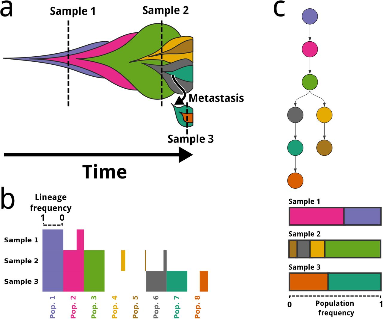
Probability that sub-tree containing given number of populations will have population frequencies ηks < 1% for all populations k in the sub-tree across all cancer samples s, computed using properties of Dirichlet distribution. A sub-tree consists of a subset of nodes from the full-tree and all edges between those nodes. By this definition, all subclones are sub-trees, but a sub-tree need not be a subclone.
To complement the above analysis concerning lone populations, we will also examine the probability of simulated trees containing sub-trees that consist entirely of populations whose frequencies are less than ϵ = 0.01. We define a sub-tree to consist of a subset of the full tree’s nodes, as well as all edges between them, ensuring the sub-tree is connected. Thus, a sub-tree can correspond to a subclone (Section 3.1), but is more general in that may omit parts of the subclone defined by the ancestral population at the root of the sub-tree. For this analysis, we did not conduct an empirical examination of the simulated data, but used only theoretical results derived from the Dirichlet distribution properties. Given a complete tree composed of K populations as well as the root node 0, and a sub-tree composed of populations T ⊆ {0, 1, …, K} with size |T|, we have in cancer sample s the result

Note that if the sub-tree T = {j} ∪ {k|k is descendent of j}, then T is equivalent to the subclone with the previous j at its head, and  . By using the Dirichlet’s marginal beta distribution, as in the previous analysis, we can compute the probability of the arbitrary sub-tree T consisting exclusively of populations whose summed frequencies across cancer samples are small, such that
  for every cancer sample s (Fig. 12). For instance, in the 100-subclone, single-sample case, we have a 6% probability of an arbitrary eleven-population sub-tree having a near-zero population frequency sum. With |T| populations in such a sub-tree, there are (T + 1)! orderings of nodes in the sub-tree that would permit nearly equal tree-constrained subclonal frequencies, and thus nearly equal tree likelihood. In the eleven-population case, there would thus be (11 + 1)! = 4.79e8 solution trees resulting from this single ambiguous sub-tree.
To compute the probability of observing such a case in the simulated trees, we must first consider how many linear chains of J populations exist in a tree with K nodes, as each has an equal chance of being assigned these small frequencies. If a tree is fully linear with no branching, there would be (K + 1)−J + 1 chains of J nodes, such that our chain of 11 populations in a 100-subclone tree would have 101−11+1 = 91 sub-trees, assuming that tree was fully linear. This in turn yields a (100% – 6%)91 = 0.36% chance that we would not observe any near-zero-frequency 11-population chains in our tree—i.e., with near certainty, we would encounter such a chain. Any degree of branching in a tree can reduce the number of node chains of a given length, thereby lessening the chance we would see this scenario. Neverthless, the probability can remain considerable, which is another reason we omitted the many-subclones, few-samples cases from our simulated data. Amongst the settings we included, we see, for instance, that in ten-subclone, single-sample trees, 6% of five-population chains will have small population frequency sums, yielding a 35% chance that we would encounter such a case in a fully linear tree.
6.6.4 Justifying our choice of the Dirichlet parameter α for generating simulated data
In Sections 6.6.1 to 6.6.3, we saw that our choice of the Dirichlet parameter α when generating simulated data (Section 6.4.2) affects multiple aspects of simulated data.
A smaller α leads to more variance in population frequencies between samples, increasing the chance that multiple samples will make clear the proper pairwise relations between subclones.
A smaller α also leads, however, to a greater probability of observing near-zero frequencies for a population across all cancer samples, inhibiting tree-reconstruction algorithms’ attempts to infer the proper place for such populations in the tree. (We do not present results with alternative α values here, but used these analyses to inform our choice of α.)
Our chosen α = 0.1 thus achieved a compromise between three factors.
It led to sufficient variance in population frequencies between cancer samples for algorithms to benefit from having access to multiple cancer samples.
It avoided creating too many populations with near-zero frequencies across samples, which would have created excessive ambiguity.
Yet it created enough such populations so that we could evaluate how algorithms dealt with ambi-guity stemming from this source.
6.7 Clustering mutations into subclones
6.7.1 Clustering overview
Pairtree provides two mutation clustering algorithms. Both use a Dirichlet process mixture model (DPMM) and perform inference via Gibbs sampling, differing in how they define their probabilistic clustering models. Let Π = {π1, π2, …, πM} represent a clustering of M mutations into K clusters, with πi indicating the assignment to a cluster of mutation i, such that πi ∈ {1, 2, …, K}. Each cluster corresponds to a genetically distinct subclone. By virtue of using a DPMM, K is not fixed, but instead inferred from the data.
Let x represent the mutation read count data. From these, we will define the posterior distribution over clusterings

Each clustering model defines its own likelihood p(x|Π), but uses the same clustering prior p(Π). The clustering prior draws on the DPMM concentration hyperparameter α, representing the cost of placing a mutation in a new cluster relative to adding it to an existing cluster. For K clusters over M mutations, with nk mutations in cluster k, we define

Both clustering models use Gibbs sampling, such that each clustering iteration resamples the cluster assignment of each mutation individually, conditioned upon the assignments of all other mutations. Thus, we wish to compute  , where πi indicates the cluster assignment of mutation i, Π is the cluster assignments of all mutations including i, and
  represents the cluster assignments of all mutations excluding i, such that
  .
.
By representing the data associated with all mutations except i with  , we get

In Eq. (28), we use Eq. (27) to establish

To complete Eq. (28), we need only define  . We leave this definition to the clustering models described in Section 6.7.2 and Section 6.7.3. Once this factor is defined, we can compute
  because we have in Eq. (28) a quantity proportional to it.

We use this definition to perform Gibbs sampling, as described in Section 6.7.4.
6.7.2 Clustering mutations using lineage frequencies
For each mutation i in each cancer sample s, we have a variant read count Vis, reference read count Ris, total read count Tis = Vis + Ris, and probability of observing the variant allele ωis. To cluster mutations using lineage frequencies, we first define for each mutation m in each cancer sample s an adjusted total read count  . Thus,
  represents the (potentially fractional) number of reads originating from the variant allele across all cells, regardless of whether the reads include mutation m on that allele. The complete data likelihood is then defined using the following notation:
S: number of cancer samples
K: number of clusters
M : number of mutations
ϕks: subclonal frequency of cluster k in sample s
Ck ⊆ {1, 2, …, M}: set of mutations assigned to cluster k, with Ci ∩ Cj = ∅ for all i and j
This yields the complete data likelihood
 with
with  . Strictly speaking, as
  may take a fractional value, it may not be a valid parameter choice for the binomial. Nevertheless, for computational convenience, we compute the integral over the binomial using the beta function, which allows for continuous
  values. Consequently, we have

By Eq. (30), we need only define  to complete the definitions required for Gibbs sampling. This follows easily from Eq. (31), yielding

This allows us to proceed with Gibbs sampling, as described in Section 6.7.4.
6.7.3 Clustering mutations using pairwise relations
As an alternative to clustering with lineage frequencies, we can cluster mutations using the pairwise relations described in Section 6.1. To do so, we compute the posterior distributions over pairwise relations for every pair of individual variants A and B, rather than the supervariants defined from an established clustering that are used for tree search. Computing the pairwise posterior distributions over relationships MAB necessitates that we first redefine the pairwise prior described in Section 6.1.6 to permit non-zero mass on the coincident relationship. For this, we allow the user to set a constant P representing the prior probability that mutations A and B are coincident, with  cancer samples by default,

We define p(Mab ≠ coincident|x) = 1 − p(Mab = coincident|x). After computing these pairwise relation posteriors for every mutation pair (a, b) ∈ {1, 2, …, M} × {1, 2, …, M} with a > b, we can define the clustering data likelihood as

As we consider every pair (a, b) without also including the pair (b, a), there are  factors in the product for M mutations. This notation relies on the indicator function

From this, we can define  , completing the definitions required for Gibbs sampling.

Thus,  is a product over the S cancer samples and M − 1 pairs that include mutation i. This allows us to proceed with Gibbs sampling, as described in Section 6.7.4.
6.7.4 Performing Gibbs sampling
Pairtree clusters mutations using Gibbs sampling, drawing on the probabilistic framework given in Eq. (30), and the lineage frequency likelihood Eq. (32) or pairwise relationship likelihood Eq. (34). The primary advantage of the lineage frequency model is that, unlike the pairwise model, it does not require the time-intensive computation of the pairs tensor before clustering can begin. The pairwise model, conversely, can be easily applied to data types other than bulk sequencing that can be represented within the pairwise relation framework, such as single-cell sequencing.
By default, the algorithm runs a total of C chains, with C set to the number of CPU cores present on the system by default, and P = C executing in parallel. Both P and C can be customized by the user. Each chain takes 1000 samples by default, which can also be changed by the user. Unlike the tree search algorithm, the clustering algorithm makes no attempt to discard burn-in samples from each chain. As tree search relies on a single clustesring common to all trees, we select the clustering result with the highest posterior probability as the algorithm’s output. Nevertheless, the user could easily adapt the implementation to represent different possible clusterings alongside their posterior probabilities, conferring insight into multiple possible solutions.
The lineage frequency and pairwise relationship clustering models use different clustering initializations, purely as an implementation artifact. The lineage frequency models simply assigns all variants to a single cluster. Conversely, the pairwise relationship model places each variant in a separate cluster. Alternative, the pairwise model also permits the user to specify an initial clustering to use for initialization. In this case, user-specified clusters can be merged, but will never be split, such that the user can force multiple variants to always remain in the same cluster.
Two hyperparameters affect clustering results. The first, α, is used in Eq. (27), with higher values corresponding to an increased number of clusters. Let  be the value provided by the user as input to the algorithm. Given a dataset with S cancer samples, The α value used in Eq. (27) is computed from this as
  , with
  by default. Representing α on a logaritmic scale via
  makes representing especially large or small values of α more convenient for the user, while scaling it with S ensures that the algorithm’s preference for placing data points in new clusters is unaffected by the magnitude of posterior weight contributed by data likelihood factors—i.e., each cancer sample-specific likelihood is effectively weighted by its own
  prior factor in computing the posterior. Finally, to prevent numerical issues, we force α ∈ [exp(−600), exp(600)].
The second clustering hyperparameter is P, the prior probability of two mutations being coincident (Section 6.7.3). Similar to how the α parameter is specified, the algorithm ensures that the number of cancer samples S does not affect the algorithm’s preference for starting new clusters by taking as input  , with
  . By default, we take
  , such that we enforce a uniform distribution over the four possible pairwise relations for each cancer sample.
6.8 Quantifying intratumor heterogeneity of cancer samples
6.8.1 Using subpopulation frequencies to reflect ITH
The subpopulation frequencies (Section 6.3.1) Pairtree fits to each tree provide a convenient means of quantifying intratumor heterogeneity (ITH) using information entropy. Because a cancer sample’s subpopulation frequencies H = {ηks} sum to one, they can be understood as a categorical probability distribution over subpopulations. These subpopulation frequencies only sum to one, however, when the non-cancerous founding population 0 is included, however, such that

As we want to exclude this non-cancerous population when examining ITH, we define re-normalized, cancer-specific subpopulation frequencies

This perspective gives rise to three metrics: the clone diversity index, the clone-mutation diversity index, and the Shannon diversity index.
6.8.2 Defining the clone diversity index
The clone diversity index (CDI)  for a cancer sample s is simply the entropy of the
  subpopulation frequencies in that sample. Thus, for K subclones, we have

Intuitively, the CDI reflects how uncertain an experimenter would be in subpopulation identity if she selected a cancer cell at random from a cancer sample, with higher  values reflecting that a cancer sample is composed of a more diverse mixture of subpopulations. The maximum CDI of log K is reached when all subpopulations are present in a cancer sample in equal proportions.
6.8.3 Defining the clone-mutation diversity index
The clone-mutation diversity index (CMDI)  extends the CDI to capture information not only about ITH, but also the tumour-mutation burden (TMB) borne by the clones in that sample. As established in Section 6.2.1, every subpopulation k has a mutation cluster Ck representing mutations that arose on the evolutionary path between k and its parent. All descendants of k inherit its mutations. Thus, the full set of mutations Mk possessed by a subpopulation k consists of

For each Mk mutation set, we can create a conditional discrete uniform distribution p(m|k), such that
 where |Mk| represents the number of mutations in the associated set.
Using this, we can create a joint distribution over subpopulations and mutations p(k, m), defining

The CMDI is then the entropy of p(k, m), such that

The CMDI reflects how uncertain an experimenter would be in subpopulation and mutation identity, if she selected a cancer cell at random from a cancer sample, then selected a mutation at random from within that subpopulation. Higher CMDI values reflect that a cancer sample is composed of a more diverse mixture of subpopulations, and/or that the subpopulations composing it bear a higher mutation load. This higher mutation load may occur because the subpopulations themselves have many mutations that occurred on the evolutionary path from their parent to them, or because the subpopulations occur deep within the clone tree, such that they have many ancestors whose mutations they inherited.
6.9 Impact of the infinite sites assumption
To simplify subclonal reconstruction, algorithms make the infinite sites assumption (ISA), which posits that each genomic site is mutated at most once during the cancer’s evolution. This implies that the same site can never be mutated twice by separate events, and that it can never return to the wildtype. Though violations of the ISA occur in cancer [26], prompting development of algorithms that permit limited relaxations of the ISA [37–39], it remains broadly valid. Under this assumption, the cancer phylogeny is a perfect phylogeny, such that descendant subclones inherit all the mutations of their ancestors. Critically, the ISA allows us to characterize more subclones than we have tissue samples.
Given complete genomes for each cancer cell, a perfect phylogeny can be constructed in linear time [40], with mutations that deviate from the ISA detected via the four-gamete test [28]. However, the bulk-tissue DNA sequencing data commonly used today do not provide complete genomes. Instead, the samples consist of mixtures of different subclones, rendering NP-complete the construction of a perfect phylogeny consistent with the exact cellular frequencies of mutations across multiple samples [22]. Nevertheless, the ISA implies relationships between mutation frequencies that can assist subclonal reconstruction. Firstly, mutations in ancestral subclones must always have cellular frequencies at least as high as those in descendent subclones, across every observed tissue sample. Secondly, two mutations on different tree branches can never have frequencies that sum to greater than one in any sample.
6.10 Multiple trees are often consistent with observed data, which Pairtree can accurately characterize
When building trees, algorithms draw on the lineage frequencies of constituent subclones across tissue samples and relationships between these frequencies to determine possible tree structures. Thus, to assess method performance on simulated data, we can enumerate all tree structures consistent with the true lineage frequencies used to generate the data, yielding a distribution over trees. This distribution will include the true tree used to generate the data, as well as any other tree structures that are also consistent with the lineage frequencies. A perfect method would be able to recover this distribution exactly, despite being given only noisy estimates of the true lineage frequencies via the observed mutation frequencies. To evaluate a method, we can then determine the extent to which its tree distribution matches the true distribution of all trees consistent with the true lineage frequencies.
Amongst our 576 simulated datasets, if only one tissue sample is provided, there are usually multiple trees consistent with the data (Fig. 8a), regardless of how many subclones are in the tree. This reaches an extreme in our ten-subclone, single-sample simulations, when there are a median of trees consistent with each dataset. This illustrates the importance of understanding uncertainty in these reconstructions, rather than simply producing a single answer (Section 3.11)—the perfect method should represent all of these trees as being equally consistent with the data, such that the user should have no reason to prefer any one structure over the others. Drawing on more tissue samples reduces this uncertainty, with most ten-sample datasets possessing only a single possible tree across the three-, ten-, and 30-subclone settings (Fig. 8a). With 100 subclones, ten samples still permits little uncertainty, with the number of possible trees rarely exceeding ten. Note, however, that in this simulated setting, multiple samples are likely to be more powerful than they would be for real cancers. Here, each sample had its lineage frequencies generated independently from other samples, increasing the chance that the sample induces tree structure constraints because its frequencies are different from all other samples. In reality, samples are likely to have correlated frequencies, given that they may be taken from similar spatial or temporal sites in the cancer that have similar population proportions.
By computing the entropy of tree distributions, we can characterize how many high-confidence trees exist in the distribution. Effectively, the entropy is a posterior-weighted count of the number of trees, with the weights in the true tree distribution being uniform because all solutions are equally consistent with the data. To determine how many high-confidence solutions was Pairtree was finding relative to the number of possible solutions, we compared Pairtree’s tree entropy for each simulated dataset to the entropy of the true tree distribution (Fig. 8b). Pairtree’s entropy generally tracked the true entropy well, suggesting that Pairtree’s uncertainty was usually consistent with the uncertainty in the true tree distribution. Notably, in settings where the number of tissue samples was higher than the number of subclones, there was only ever one true tree (Fig. 8a), while Pairtree’s tree distribution entropy exceeded the true distribution’s entropy by more than 5.9 × 10−6 bits with only one exception across 181 simulations (Fig. 8b). These results demonstrate that, when the data is sufficiently high-resolution as to permit only a single solution, Pairtree finds only a single solution.
Though examining tree distribution entropies reveals the number of high-confidence trees Pairtree finds, it says nothing about the quality of those trees. To gain further insight, we can view a distribution over trees as inducing a distribution over the parents of each subclone. For a given dataset, to compare the Pairtree-computed tree distribution to the distribution of trees consistent with the true lineage frequencies, we can consider the joint Jensen-Shannon divergence between parent distributions induced by these tree distributions, normalized to the number of subclones in the tree such that the divergence will always lie between zero bits and one bit. We refer to this metric as the parent JSD. Even if the tree distributions have no overlap—which could occur, for instance, if there is only a single true tree that Pairtree fails to locate—the parent JSD nevertheless allows the distributions to have a small divergence if they agree on parent choice for most subclones. We see that the parent JSD falls as the number of samples increases for a given number of subclones (Fig. 8c), suggesting that Pairtree can efficiently exploit the constraints provided by additional tissue samples to produce higher-quality trees. Moreover, when the number of samples exceeds the number of subclones such that there is only one tree consistent with the true lineage frequencies (Fig. 8a), the parent JSD is effectively always zero, complementing the tree entropy analysis (Fig. 8b) to show that the one tree Pairtree finds is almost perfectly consistent with the true tree. Additionally, when the pairwise relation error is examined at a more granular level (Fig. 8d), we see that for a given number of subclones and samples it is always less than the parent JSD. This suggests that, even when Pairtree doesn’t perfectly determine the parents of each subclone, the distributions over relationships between subclones (e.g., ancestor-descendant or on-different-branches) are closer to the truth. The quality difference between pairwise relation distributions and parent distributions is stark for the 100-subclone setting. Though Pairtree only rarely finds the correct parents, demonstrated by the parent JSDs that are close to one (Fig. 8c), the pairwise relation errors are much lower (Fig. 8d), indicating that the higher-level relationships between subclones are closer to being correct.
6.11 Failings of existing algorithms
Given that the algorithms we compared against often failed to produce results on our simulated datasets, considering possible reasons for this poor performance is a worthwhile exercise. We hypothesize that CITUP attempted to enumerate all trees with a given number of subpopulations, but faced too many trees to make this approach feasible when provided with more than three subpopulations.
PASTRI attempted to overcome the difficulties of enumeration by first sampling lineage frequencies, then enumerating only trees consistent with those frequencies. The PASTRI implementation is nevertheless limited to 15 subpopulations [35]. Even with ten subpopulations or fewer, because PASTRI samples frequencies without considering tree structure, the frequencies are often inconsistent with any tree when the algorithm is given many tissue samples, as the frequencies collectively impose constraints that rule out all possible trees. A weakness of this approach becomes apparent in real cancer datasets, where new subpopulations often emerge when they acquire driver mutations that confer a strong selective advantage, leading to them displacing their parents such that the lineage frequency of the child is only slightly greater than that of the parent. Indeed, this situation often occurs in the leukemias considered here. As PASTRI samples lineage frequencies before enumerating consistent trees, the frequencies sampled for children in this situation will often by chance be slightly higher than their parent, rendering the correct tree structure impossible to recover.
LICHeE fared better than CITUP and PASTRI, as it first constructed a directed acyclic graph (DAG) containing possible trees permitted by the noisy subclonal frequency estimates provided by the VAFs, then only considered spanning trees of this graph [18]. However, this approach could not scale to most 100-subpopulation trees, presumably because the corresponding DAGs have too many spanning trees. Even in settings with thirty or fewer subpopulations, LICHeE exhibited considerably higher error than Pairtree both with respect to lineage frequencies and pairwise relations, despite us computing lineage frequencies for LICHeE’s tree structures using the same algorithm as Pairtree. This suggests that the DAGs did not include as spanning trees good tree candidates, or that the error scoring function LICHeE used to indicate tree quality did not properly reflect tree quality. Some of LICHeE’s shortcomings may have arisen because it takes as input only VAFs, rather than mutation read counts. Consequently, LICHeE has no knowledge of how precisely the VAFs should reflect underlying subclonal frequencies, unlike methods such as Pairtree that use a binomial observation model.
In general, stochastic search algorithms are a superior approach relative to exhaustive enumeration methods when faced with numerous subpopulations, since they avoid the exponential growth in number of trees as a function of number of subclones [21]. For stochastic search algorithms to work well, they must locate high-probability regions of tree space and limit their search to those areas. However, as data become richer, tree space is rendered more complex, such that existing search algorithms struggle to navigate through it. This was apparent with PhyloWGS, which consistently exhibited higher error for many-tissue-sample simulations than few-tissue-samples ones. By constructing the pairs tensor and using this as a guide to tree search, Pairtree is better able to cope with many tissue samples and the constraints they impose.
Footnotes
References


