

Abstract
Predicting the response of the cortical microcircuit to perturbations is a prerequisite to determine the mechanisms that mediate its response to stimulus; yet, an encompassing perspective that describes the full ensemble of the network’s response in models that accurately recapitulate recorded data is still lacking. Here we develop a class of mathematically tractable models that exactly describe the modulation of the distribution of cell-type-specific calcium-imaging activity with the contrast of a visual stimulus. The inferred parameters recover signatures of the connectivity structure found in mouse visual cortex. Analysis of this structure subsequently reveals parameter-independent relations between the responses of different cell types to perturbations and each interneuron’s role in circuit-stabilization. Leveraging recent theoretical approaches, we derive explicit expressions for the distribution of responses to partial perturbations which reveal a novel, counter intuitive effect in the sign of response functions. Finally applying the theory to inferring feedback to V1 during locomotion, we find that it is predominantly mediated by both SOM and VIP modulation.
Introduction
A defining feature of the operating regime of cortex is strong recurrent excitation that is stabilized and loosely balanced by recurrent inhibition1–6. This understanding was achieved through the discovery of a fundamental link between circuit stabilization and the response to specific perturbations, and was established in minimalistic recurrent network models with only two units, one describing the mean excitatory activity and another describing the mean activity of a single inhibitory type1,7. In these models, when recurrent excitation is sufficiently strong and stabilized by inhibition, an increase in the input drive to the inhibitory population elicits a simultaneous decrease of the excitatory and, paradoxically, of the inhibitory steady-state activity. This link provided a proxy to test inhibition stabilization in in vivo cortical circuits and an understanding of counter-intuitive responses to perturbations1–4. Nevertheless, and despite successful predictions, our understanding of the implications of the circuit’s response to specific perturbations is still at its onset.
First, there is little consensus on how to generalize the fundamental link between stabilization and response to perturbations to the case of multiple inhibitory types8,9. The inhibitory sub-circuit is composed of multiple elements with three types – parvalbumin-(PV), somatostatin-(SOM), and vasoactive-intestinal-peptide (VIP) expressing cells that constitute 80% of GABAergic interneurons in the mouse primary visual cortex (V1)10. Importantly, these interneurons form a microcircuit characterized by a specific connectivity pattern 11–13, but how the stabilization of strong recurrent excitation is implemented by these interneurons and whether the structure in the synaptic connectivity in any way constrains the circuit’s response to perturbations is not understood. Second, viral (but not transgenic) cell-type specific optogenetic perturbation is insufficient to elicit a paradoxical response4,14, demonstrating that minimalistic models are insufficient to account for the response to concrete optogenetic manipulations and highlighting the need to advance the theoretical understanding of the circuit’s response to perturbations in more detailed models of cortical activity in which cell, cell-type, and perturbation diversity play a role. Finally, if new models hope to account for this emerging complexity, they will be rife with parameter degeneracy. Yet, a data-driven framework designed to sub-select from the universe of such models has not been established. As biological realism increases, making parameter-independent predictions or even locating the parameters that situate a biologically insightful model in the correct network state becomes exponentially difficult.
Here we developed a program for inferring high-dimensional cell-type-specific network models from data and a theoretical framework for the quantitative prediction of the circuit’s response to patterned optogenetic perturbations. This framework allowed us to i) find a mechanism for network control based on hidden symmetries in the response matrix ii) link stability and response in high-dimensional multi-cell-type circuits, iii) predict an unexpected effect to partial perturbations and iv) infer which are the inputs that would induce changes in the network activity akin to those induced by behavioral modulations. Specifically, we analyzed calcium-imaging recordings of the activity of each interneuronal type in the visual cortex of the awake mouse, in response to stimuli of increasing contrast while the mouse was in a stationary condition. We identified, via a combination of fitting methods and theoretical tools15–17 a family of mathematically tractable high-dimensional models that exactly describe the distribution of cell-type-specific calcium-imaging activity and its dependence on the stimulus contrast. Using recent results in random matrix theory18, we defined an approximation that allowed us to obtain explicit expressions for the mean and variance of the distributions of responses to patterned optogenetic perturbations of the high-dimensional models. By linking the mean responses of these distributions to the response to perturbations in simpler, more minimalistic models and by evaluating these expressions with the parameters of the models fit we were able to make quantitative predictions. We report that our fitting method, remarkably, provides sets of parameters endowed with key aspects of the structure of the connectivity matrix found in the mouse visual system11,19. By studying mathematically the implications of this structure for the response to population-wide cell-type-specific perturbations, we predict a parameter-independent symmetry between the responses induced by perturbation of VIP or of SOM, two interneuron types involved in a disinhibitory micro-circuit whose competition directly regulates pyramidal cell activity. We find that this hidden symmetry principle is respected with remarkable reliability in the models that fit the data. Furthermore, we establish a mathematical link between cell-type-specific response to perturbation and sub-circuit stability. By implementing those insights in these data-compatible models we provide new evidence, aligned with convergent experimental20 and theoretical9 arguments, that PV interneurons play a major role in circuit stabilization. Furthermore, we find that when effecting cell-type-specific partial perturbations, the fraction of cells that respond paradoxically has a non-monotonic dependence on the fraction of stimulated cells. There is a range in which increasing the number of stimulated cells actually decreases the fraction of paradoxically responding cells, yielding a fractional paradoxical effect that can be linked to the loss of circuit stability in the context of partial perturbations, opening a new avenue for experimental inquiry. Finally, we reveal the mechanism by which locomotion affects V1 by inferring the distribution of inputs that each cell-type population would need to receive for the network response to mimic the effect of locomotion.
Results
The analysis of low-dimensional (LD) models, in which there is one unit per population, revealed that the response to controlled perturbations could be interpreted to characterize the operating regime of cortex1,7. This was established in models that considered only two populations, excitatory and inhibitory. In these models, the circuit’s response to perturbations is linked to its stability (see Eq. (S11)). When recurrent excitation is strong and stabilized by inhibition (an inhibition-stabilized network or ISN), an increase in the external input drive to the inhibitory population results in a paradoxical decrease of its steady-state activity. Conversely, a paradoxical response can only be observed in ISNs, and can therefore be utilized as a proxy to experimentally assess the stabilization properties of the cortical circuit4.
Cortical circuits in vivo are composed of multiple inhibitory types and generate broad distributions of activity. In models that account for these features, the paradoxical response of a given inhibitory cell-type is not a predictor of the ISN condition21 and its implications for circuit stabilization are not understood8. Here, we set out to establish a framework (Fig. 1) that enables quantitative, cell-type specific predictions of the response to perturbations in models that that incorporate the diversity of inhibitory cell-types and are high-dimensional (HD), meaning that there are many units per population that may be heterogeneous in connectivity and in other properties.

Top: Model inference stage. In high-dimensional models with multiple cell types, the response of the circuit to perturbations is strongly dependent on parameters. In order to build models with predictive power, we fit the distribution of activity of each cell-type population (E, PV, SOM and VIP) to cell-type specific calcium imaging data of mouse visual cortex in response to stimuli of different contrasts, in a stationary condition (see also Fig. 2). Given a certain accuracy of the fit, we work with a family of data-constrained models. Middle: Response to perturbations stage. We developed a theoretical framework that allows us to derive explicit expressions for the mean and the variance of each cell-type population response to perturbations, under a suitable approximation. This approximation allows us to map the insights obtained in the perturbations analysis in LD models to HD models (see also Fig. 3). Bottom Left: Hidden response symmetries. We find hidden symmetries in the response to perturbations that lead to two mutually-exclusive mechanisms for network control via the manipulation of SOM and VIP activity (see also Fig. 4). Bottom middle left: Stability and response. Building the mapping between LD and HD models, we link the mean response to full-population perturbations with the stability of the network sub-circuit without the perturbed cell-type population, extending results of LD models with a single inhibitory type (see also Fig. 5). Bottom middle right: Partial perturbations. When the perturbations to the circuit are restricted to a subset of neurons, the responses to perturbations are bimodal. If a full population perturbation induces a paradoxical effect, we show that a partial perturbation exhibits a fractional paradoxical effect (see also Fig. 6). Bottom right: Modulation inference. Finally, we infer the perturbation pattern that would elicit a model response that matches the activity modulation induced by locomotion (see also Fig. 7).
Mean-field theoretical approach to model high dimensional data
We study the response to visual stimuli of varying contrast in neurons of layer 2/3 of primary visual cortex (V1) of awake, head-fixed mice. Specifically, we study the responses of Pyramidal (E) cells and of Parvalbumin (PV), Somatostatin (SOM) and Vasoactive Intestinal Polypeptide (VIP)-expressing interneurons while the animal is shown square patches of drifting grating stimuli of a small size (5 degrees) at varying contrast.
To describe contrast modulations observed within each cell-type population, we build HD models with different proportions of cells in each population as measured experimentally10. To infer the model parameters, we begin by first inferring the parameters of a LD circuit with four units, each representing the mean activity of one cell-type population (Fig. 2a, fitting pipeline). Each unit has a power-law input-output function22. All four cell-types receive a baseline input to account for the spontaneous activity observed, while feed-forward inputs only target the E and PV populations and are taken to be a linear function of contrast. To simultaneously find the synaptic connectivity parameters, the value of the baseline inputs, and the values of the stimulus-related inputs, we construct surrogate contrast-response curves for each cell-type by starting with the measured mean response of each cell type at each contrast, and adding Gaussian noise to each of these data points, with mean zero and standard deviation given by the standard error of the given data point. We fit each LD model by finding the non-negative least squares (NNLS)23,24 solution to each surrogate data set, and select from these, hundreds of data-compatible model parameters for which the network steady-states provide the best fit. Starting from these seed parameters, we search over the parameters of the HD model to find those HD models that match well the experimentally measured distributions of responses of all of the cell types (see below and Fig. 8). In HD models (Fig. 2b), each neuron has a power-law input-output function22,25 and receives heterogeneous baseline inputs and a stimulus-related inputs that have cell-type-specific means and variances (and the means of stimulus-related input depend on the stimulus). The connectivity is heterogeneous with a mean and a variance dependent on both the pre-and post-synaptic cell-type. This class of models reduces to the LD class whenever there is no heterogeneity in the connections or the inputs (homogeneous network).

a) Model inference pipeline. We firstly fit the mean activity of the pyramidal-cell (E, black), PV (turquoise), SOM (orange) and VIP (pink) populations, as measured with two photon calcium imaging (thick line, ± s.e.m.), as a function of stimulus contrast with a LD model of four populations. Inputs to each cell-type are composed of a spontaneous activity baseline hb, and a stimulus related current, hc, to E and PV, modeling the feed-forward inputs from layer 4. Stimulus-related inputs are linear functions of the stimulus contrast. After performing non-negative least squares (see text) to find the 22 parameters of the model (16 weights, 4 baseline inputs and 2 stimulus-related inputs) we find a family of possible models (thin lines, mean and s.e.m. over models; here we show the 300 models) that qualitatively reproduce the mean activity. We aim to find a family of HD models that recapitulate not only the means but the entire distributions of activity of all cell-types at all contrast values. Then, we use the inferred LD model parameters as a seed to build Gaussian priors for the connectivity mean (wαβ) and the input means ( and
and  ), whereas priors for the variance of the connectivity and the inputs are chosen arbitrarily. We generate HD models by sampling from those prior distributions of parameters, and compare the obtained model distributions to the fitted data distributions using an error function. This error, is given by the sum of the Kullback-Leibler divergences of the distributions given by the model (Pmf) and the data (Pc) for all cell-types and contrast values, which can be found explicitly. By only accepting models with error less than a threshold of 0.5 (top 0.005%), we build a family of suitable models. b) HD model has a distribution of external baseline inputs with mean Hb, and a stimulus related current, Hc, to E and PV, which is a linear function of the stimulus contrast. The variance of the input does not depend on contrast. The model has 34 parameters (24 that account for the 16 mean weights and the 8 low-rank weight variance, 4 mean baseline inputs, 2 mean stimulus-related inputs and 4 input variances, independent of contrast). For more details see Figure 8. c) Distribution of KL divergences, indicating the 0.5 threshold. We used models below this threshold for the analysis in the remaining text (see Methods for details). d) Example of a parameter configuration within the threshold. Data (histogram, colored bars) and data fits (solid colored line) are in good agreement. e) Distribution of mean connectivity weights over all possible models is shown. The gray-scale background of each panel is the logarithm of the mean of each distribution. Notice that, as in experiments (see Fig.9), the models lack recurrent SOM and VIP connections, and the connections from VIP to E and PV are small on average.

In order to study perturbations in HD models (top left), in which the heterogeneity in the connections and the inputs induces heterogeneity in the response gain of each neuron, we make an approximation. By linearizing around the homogeneous fixed point (i.e. linearizing around the fixed point of the network without heterogeneity, middle panel), we are able to leverage results from random matrix theory to obtain explicit expressions for the mean and the variance of the response of each cell-type population. The analytical approach reveals that, when perturbing all cells in a given population, the mean response of an HD system in the HFA is equal to the response of the LD system (right panel, which is equivalent to the system without heterogeneity).

a) A parameter-independent relation holds true between the response of pyramidal cells (E), PV interneurons (P), SOM interneurons (S), and VIP interneurons (V) to perturbation of SOM and VIP. These relations or hidden response symmetries (HRS), described by Eq. (1), are derived for LD models under the assumption of VIP projecting only to SOM, and hold for the mean response of HD models under the HFA. The illustration depicts the response of cell-type α to VIP perturbation vs the response to a SOM perturbation multiplied by the coefficient in Eq. (1). Given a perturbation to the VIP population, the constraints imposed by the HRS define the sign and magnitude of the response to SOM, so that possible values lie on a line, as shown. Two regimes can be identified: One in which VIP disinhibits while SOM inhibits the cell-type α (lower right, green) and another one in which the opposite is true (upper right, purple). We hypothesize that this relation could approximately hold at the single cell level. b) Distribution of responses to full-population SOM (left) and VIP (right) perturbations, for maximum stimulus contrast. Green histograms are the result of the simulation of a fully nonlinear HD system, while colored histograms and corresponding lines are the analytical result, only possible under the HFA. c) Opposite and proportional responses to perturbations of SOM and VIP, for E (top left), PV (top right), SOM (bottom left) and VIP (bottom right), for the top 360 of models. Given that the data-compatible connectivities have only small values of connections weights from VIP to E, PV and SOM, this symmetry is evident in the models that fit the data. These results show that the best fit models support a clear disinhibitory motif in which a perturbation to VIP decreases SOM activity and increases both E and PV, and a perturbation to SOM does the opposite. d) Hidden response symmetries at the single neuron level. Responses of single cells of type E (black), PV (turquoise) and SOM (orange) and VIP (pink) cells to a VIP perturbation, vs. the responses of those same cells to a SOM perturbation multiplied by the factor:  . The response symmetries hold at the single cell level in the fully nonlinear HD system. In experiments, it may be necessary to compare the response of one cell to a SOM perturbation and a different cell to a VIP perturbation. The contour lines show the distribution of such responses across pairs of cells, with VIP perturbed for one and SOM perturbed for the other. In this case, the response to VIP and to SOM perturbations are not perfectly correlated, but the two perturbations still elicit responses with opposite sign.

a) Graphic summary of the relation between stability and paradoxical responses. The response of a cell-type α in the LD case, which is the change in activity normalized by the size of the perturbation, is shown as a function of contrast. When the response of the cell-type which is being perturbed is negative, the response is paradoxical. A paradoxical response of a cell-type in an LD model in turn implies that the circuit without that cell-type is unstable (see Eq. 2). This relation holds in the HD system under the HFA if the variance of the weight distribution is sufficiently small. b) Distribution of responses to full-population perturbations for a stimulus of 100% contrast. Green histograms are the result of the simulation of a fully HD nonlinear system (dashed green line is its mean), while colored histograms and colored lines are the analytical curves obtained under the HFP approximation (dashed red line is its mean, corresponding to the LD system response). The responses of E, SOM and VIP cells are not paradoxical, while all cells in the PV population respond paradoxically to PV stimulation. c) Eigenvalue distribution of the Jacobian of the sub-system without the E (top left), without the PV (top right), without the SOM (bottom left) and without the VIP (bottom right) populations. As the outliers of the eigenvalue spectrum of the Jacobian under the HFA are defined by the LD system for sufficiently small variance of the weight distribution, and because  , a mean negative response in the HFA approximation indicated that the sub-circuit without that population is unstable. In the special case in which VIP projects only to SOM, the lack of a paradoxical response in SOM indicated that the E-PV circuit is stable. d) Cumulative distribution of responses (HFA) to full-population perturbation in the presence of a visual stimulus for varying stimulus contrast. e) Mean response of each cell type to a perturbation to that same cell type, vs the real part of the maximum eigenvalue of the sub-circuit without that cell type, for all values of the contrast. f) Mean response of each cell type to a perturbation to that same cell type as a function of contrast, for models in the HFA (E in black, PV in turquoise, SOM in orange, VIP in pink) and for the fully nonlinear network (green). g) Same as f) for the standard deviation of the response. Note the paradoxical response of PV at all contrasts and the non-paradoxical response of SOM in most cases. In the multiple cell-type circuit and unlike in the EI system, excitatory activity can in principle also respond paradoxically. Nevertheless, none of the data-compatible models obtained had an excitatory paradoxical response.

a) Top: distribution of perturbation strengths, when perturbing 25% (left), 75% (middle) and a 100% (right) of the PV population. This can be understood as having an increasingly larger radius of an optogenetic stimulus, as indicated in the top right scheme of a mouse brain. Middle: Partial perturbations result in a bimodal distribution of responses in the HFA, given by a mixture of two Gaussians (turquoise). The rightmost peak (dashed red) corresponds to the response of the sub-population of stimulated PV cells, while the leftmost peak (dashed green) corresponds to the response of non-stimulated PV cells. The distribution of responses is the HFA is in good agreement with simulations of the fully nonlinear system (gray histograms), for this example model at lowest contrast. Note that the mean response of the perturbed population changes sign with increasing number of perturbed PV cells. Bottom: Eigenvalue spectrum of the Jacobian of the non-perturbed sub-circuit for the HFA approximation (purple, orange and yellow) and the fully nonlinear system (green). The maximum eigenvalue of the network subsystem changes sign with increasing number of perturbed PV cells. b) Top left: Mean of the entire (bimodal) distribution of PV cell responses (turquoise), the mean of the perturbed PV cell responses (dashed red) and the non-perturbed PV cell (dashed green) responses as a function of the fraction of PV cells perturbed. Top middle: While all three means monotonically decrease with the fraction of stimulated cells, the variance of both perturbed (dashed red) and non-perturbed (dashed green) monotonically increase, resulting in a non-monotonic variance of the full distribution. Top right: Fraction of negative responses as a function of the fraction of stimulated cells shows a non-monotonic dependence, which we name the fractional paradoxical effect. Bottom: The fractional paradoxical effect is a signature of models that fit the data, and occurs for all values of the contrast. Simulations of the fully nonlinear system (green) are in good agreement with calculations from the HFA (turquoise). c) Linking response and stability across models. A fully nonlinear system can be linked to a HD system of lower complexity via the HFA. The mean response to a partial perturbation in the HFA can be mapped to the response of a PV sub-population in a LD system with two PV populations, a perturbed one (red) and an unperturbed one (green) see, Eq. (S106). d) Top: Mean response of the perturbed PV population as a function of the value of the outlier eigenvalue for different fractions of perturbed PV cells for the fully nonlinear system (green) HFA (blue colors) and the equivalent 5D system (purple orange palette). The mean responses become negative when the maximum eigenvalue crosses zero, indicating instability of the non-perturbed sub-circuit. Bottom: Mean response of the perturbed PV population as a function of the value of the outlier eigenvalue in the equivalent 5D model obtained from different models that fit the data, for different values of the contrast.

a) Distribution of △ activity (difference between each cell’s activity in the locomotion and the stationary condition) for each cell type and different values of the stimulus contrast. Stars in the top right corner indicate when mean is significantly different from zero (p<0.0001, t-test). Dashed lines indicate best Gaussian fits. Solid lines are fits from the explicit expressions (see Eqs. S113 and S111) b) Scheme of how to infer the cell-type specific perturbations (Gaussians of mean gα and standard deviation gα for α = {E,PV,SOM,VIP}) that give rise to the distribution of Δ activity (with mean μα and standard deviation Δα). By fitting these last expressions to data, the inputs can be inferred. c) Mean of Δ activity and standard deviation of Δ activity as a function of contrast. Dashed lines are the data (E in black, PV in blue, SOM in orange and VIP in dark red), with stars in matching colors when the mean is significantly different from zero (p<0.0001, t-test). Full lines indicate fits as described in b, for the family of models that fit the stationary data. The mean (g) and the standard deviation (d) of the inferred perturbation are shown in the left panels.

a) Fitting pipeline: The distribution of activity generated by a model with a power-law non-linearity and recurrent and feed-forward inputs that are Gaussian distributed has an explicit mathematical form17 (Eq. (S44)). We used it to fit that form to each of the distributions of activity for a given cell-type at a particular value of the stimulus contrast. A mean field model, with the appropriate parameters should be able to recapitulate the distributions of activity of all cell-types at all values of contrast. To find them, we generate high-D models by sampling from prior distributions of parameters given by the LD model fit (see Fig. 2), and compare them to the fitted data distributions using an error function, given by the sum of the Kullback-Leibler divergences of the distributions given by the model ( ) and the data (
 ) for all cell-types and contrast values, which can be found explicitly. By only accepting models with error less than a threshold of 0.5 (top 0.005%), we build a family of suitable models. b) Example of a parameter configuration within the threshold. Data (histogram, colored bars) and data fits (solid colored line) are in good agreement with the mean-field theory distributions (dashed gray line) and the simulations of the full high-D model (gray bar histogram).
We emphasize that, due to the nonlinear transfer function, heterogeneity in the values of the synaptic connectivity will change the mean activity compared to the system without heterogeneity. Consequently, it is not sufficient to use the parameters found for the LD model as the mean values of the heterogeneous connectivity and input distributions; the mean and variance of the connections and the inputs have to be found simultaneously for the HD model to fit the data. We expect the HD mean values to be near the LD values, so we focus our search for HD mean values on the vicinity of the LD values.
In order to find HD models, we build on two facts. First, given a power-law input-output function, there is a closed-form expression that maps the distribution of inputs that a given cell-type population receives to the distributions of activity that cell-type population produces17 (see Eq. S44). Given that this expression is explicit, it allows us to infer, from the distributions of activity for each cell-type and each stimulus contrast, the distributions of inputs to each population. Second, given a HD circuit model (for a fixed set of parameters), the distributions of inputs and activities it will produce can be computed self-consistently through mean-field theory15,16 (see Eq. S40). These two facts, taken together, allowed us to obtain an explicit error function that quantifies how different the measured distributions of activity of all cell types at all contrast are from those distributions produced by the mean-field equations with a given set of parameters. To generate candidate models, we sample from prior distributions on the parameters. These prior distributions are Gaussian distributions for the mean and variances of the weights and the external inputs. The priors for the means are centered on the LD seed parameters. We keep the solutions that have a sufficiently small error, to define a family of HD models that fit the data (Fig. 2c,d). This family of models recapitulates the dependence of the distribution of responses of all cell types on contrast, and captures both the spreading out of the distributions with increasing contrast and the heavy tails of the distributions seen in calcium data.
We require that the recurrent excitation is strong, and that the LD system has a paradoxical response in the PV population in the absence of visual stimulation (i.e. at zero contrast), as measured experimentally4. Beyond that, this optimization takes as sole input the response data and uses no other prior information on the synaptic structure, hence it is not obvious that any meaningful synaptic structure should be recoverable from such a procedure. Surprisingly, the structure of the inferred connectivity matrices has a striking resemblance to that reported experimentally (Fig. 2e), see also 9b). In particular, recurrent connections within the SOM population and the VIP population were absent in most models, as observed in mouse V111,13,19 (Fig. 9); and,whenever inputs were chosen to target only E and PV, VIP interneurons had weak or absent connections to all other cell-types except SOM interneurons, also as reported in mouse V111,13,19.
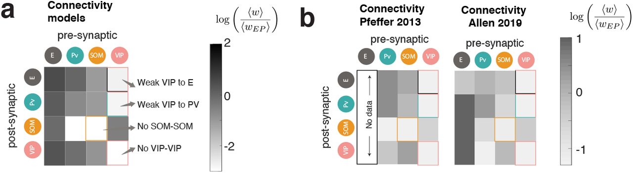
a) Mean of the distributions of weights shown in normalized by the synaptic weight from PV to E, for comparison with the available experimental data (background grayscale in panel 2e)). b) Left: Synaptic weight connectivity as obained in11. Right: Publicly available connectivity data from the Allen institute (https://portal.brain-map.org). The shown matrix is mean synaptic weight of the distribution of connections times the connection probability times the fraction of neurons belonging to the pre-synaptic cell-type, normalized by the synaptic weight from PV to E, as done originally in11. These two matrices are shown here for comparison. There is currently no agreement on the strength of the connection from PV to VIP.
Analytical approach to full and partial perturbations
To develop a theoretical framework for using optogenetic perturbations to probe the circuit, we compute the distribution of responses of the network to perturbations, e.g. optogenetic activation or suppression of sets of cells. For each pair of cells, the change in steady-state response of the cell i (belonging to a population α) per small change in the input to a cell j (belonging to a population β) will be given by the element  of the response matrix χ. We developed a theoretical framework that allows analytic computation of the mean and the variance of the response over each population to (small) perturbations, under the following approximation. We assume that the gain of the neurons in a given population is the same for each cell (equal to the gain of the homogeneous system). Our system then satisfies the assumptions needed to build on recent work on random matrix theory 18 to compute these response distributions. Under this approximation, which we refer to as the homogeneous fixed point approximation (hereinafter HFA, see Eq. S54), we are able to obtain analytical expressions for the behavior of the mean and the variance of the distributions of optogenetic responses in each population to either full or partial, and either homogeneous or heterogeneous, perturbations. Importantly, we find that under the HFA, neurons belonging to a specific cell-type’s population of the HD heterogeneous system, have a mean response to cell-type-specific perturbations given by the response of the homogeneous system without heterogeneity, equivalent to the LD system (Fig. 3, see also Eq. S121), allowing us to directly link the response of the LD and HD models. In the following, we will distinguish analytics using the HFA, from simulations of the fully nonlinear system, in which different cells of a given cell-type can have different gains at the network’s fixed point.
Symmetry principles of optogenetic response
Figure 4 shows the first application of the link between LD and HD systems offered by the HFA. When computing the response distributions to perturbations, we find consistent symmetries in the responses to perturbation of the SOM population vs. a perturbation of the VIP population. In order to understand this, based on our recovery of the structure of the connectivity matrix found in mouse V1 (Fig. 2), we examined the linear response matrix of LD circuits (Eq. S7) for a generic connectivity that satisfies the condition that VIP projects only to SOM, but is otherwise arbitrary. We found that in this case, the linear response matrix has a symmetry between the response of E, PV, SOM and VIP to a VIP perturbation vs. to a SOM perturbation: for each cell type, the two responses will be negatively proportional to one another, with a common proportionality constant across the four cell types (Fig. 4a), see also Eq. S13). In the case of VIP, there will be an additional shift given by its own gain. Specifically, if  is the gain of VIP at a particular steady-state configuration and ωSV is the synaptic weight from VIP to SOM then

We refer to these equalities as Hidden Response Symmetries (HRS) (Fig. 4a-c). Because the mean response of a population to the perturbation of all neurons in another population under the HFA is given by the response of the LD circuit (see Figure 2), these symmetries also apply to the mean of the distributions in the high dimensional system under the HFA. Figure 4b shows the response distributions of an example model from Figure 2, to perturbations of the entire SOM and VIP populations. The distributions obtained under the approximation (colored lines) are in good agreement with the results of simulations of the fully non-linear system (green). 4c quantifies to which extent the HRS hold in the mean response of HD models that fit the data, both in models under the HFA and the fully nonlinear networks. As the data-compatible models naturally exhibit only weak connections from VIP to other interneurons besides SOM, this symmetry in the mean response is revealed in this family of models.
The HRS formalize a clear intuition: Because VIP neurons only project to SOM neurons, a weak perturbation to VIP will only affect the rest of the circuit through SOM, relaying that perturbation with an opposite sign.
The HRS defines two alternative regimes of network configuration: one in which an increase in the input to VIP increases the activity of a given population, and another one in which it decreases it, with SOM causing an opposite response in each case. VIP will be inhibitory if the disinhibitory effect of SOM cells on PV cells outweighs the direct inhibitory effect of SOM cells on E cells; otherwise, it is disinhibitory. In our data-compliant models, activation of VIP has a disinhibitory effect on E, as in experiments26–29, and disinhibits PV while inhibiting SOM. These effects of small VIP perturbations on PV and SOM, and the opposing, proportional effects on E, PV and SOM of small VIP versus SOM perturbations, with the same proportionality constant for all, are conclusive predictions resulting from our our analysis.
Finally we asked to which extent the mathematical understandings offered by the Hidden Response Symmetries hold at the single cell level. We reasoned that the effect of the perturbation that each cell receives, will respect the HRS but now with the average values of the connectivity and the gains. Indeed, Figure 4d shows, for a single example fully nonlinear network, the response of each cell to a perturbation to the full SOM population vs the response to a perturbation to the full VIP population with the appropriate corrections. These responses are perfectly anticorrelated.
Paradoxical effects in circuits with multiple cell types and link to sub-circuit stabilization
We next investigated the relation between paradoxical response of an inhibitory cell-type and the stability of the network sub-circuits. A multi-cell-type circuit is an inhibition-stabilized network (ISN) if and only if an increase in the input drive to any or all of the inhibitory populations paradoxically results, in the new steady state, in a change in the same direction – both increasing, or both decreasing – in both the inhibitory input to the excitatory population and of the excitatory activity.25,30. Therefore, if a perturbation to the entire inhibitory sub-circuit elicits a paradoxical decrease in activity in all GABAergic cells that project to excitatory cells, thereby guaranteeing that the net inhibition received by excitatory cells decreases, and also decreases the excitatory activity, then the circuit is an ISN. The converse, that the ISN condition implies a paradoxical response of the inhibitory activity, is only true in an E/I circuit: in the multi-cell-type case, there are multiple ways in which the total inhibitory input current to the E population can decrease, so no specific cell-type needs to decrease its activity.
To systematically investigate the response of each cell-type to its own stimulation, we start by focusing on the diagonal of the LD linear response matrix (see Eq. S10) χαα, found by linearizing the dynamics in the vicinity of some stable fixed point of activity. These elements, can be written as a function of the Jacobian J of the entire circuit (which drives the linearized dynamics) and the Jacobian Jα of the sub-circuit without cell-type α:

At a stable fixed point, the determinant of the negative Jacobian is positive (because all eigenvalues of the Jacobian have negative real part). As a result, det(–J) > 0, so χαα has the same sign as det(–Jα). Thus, if the response of cell-type α at a given fixed point is paradoxical (χαα < 0), then the sub-circuit without that cell-type is unstable (det(–Jα) < 0, see Eq. (S10)). This insight is a simple generalization of the two-population ISN network, in which the I unit shows a paradoxical response at a given stable fixed point when the circuit without it, i.e. the E unit, is unstable, and links cell-type-specific paradoxical response to sub-circuit stability in a more general setting (Fig. 5a)). In particular, we furthermore find that when VIP projects only to SOM, the response of SOM to its own perturbation is directly linked to the stability of the sub-circuit E-PV: a paradoxical response in the SOM population indicates that the E-PV sub-circuit is unstable (see Eq. S12).
To link the LD insights to the HD models, we notice that if the connectivity is dominated by its random component (see Eq. S33), the eigenvalues of the Jacobian of the HFA will follow a circular law, except for a set of outliers corresponding to the eigenvalues of the LD system (as proven in31 for the case of an i.i.d. random matrix, see also Methods; this seems to well describe our results, but a more precise treatment of our case, in which the variances of different cell types are different, is in18). Therefore, in the HD systems, whenever the mean of the LD system is paradoxical, then for sufficiently large variance of the connectivity, the system without that population will, under the HFA, retain the unstable eigenvalue of the LD system and thus be unstable (Fig. 5a)). This phenomenon is illustrated for an example model at 100 % contrast in Figure 5b-c. Notice that the mean response is only paradoxical for PV cells, and that therefore the eigenvalue distribution of the system without PV, has a positive outlier (top left panel). For comparison, simulations of the fully nonlinear system are also shown. Although there is no theoretical guarantee that the outlier eigenvalues of the fully nonlinear system will be organized as the ones in the HFA, we observe good agreement.
To fit the HD models, we required that the LD seed used for the model priors (see Fig. 2 and Methods) had a paradoxical response in PV in the absence of visual stimulus, to match experiment4, but we did not apply any constraints to the response of the HD system, which therefore could have lacked a paradoxical response in PV. Nevertheless we observe that the mean response of PV to its own stimulation is paradoxical in almost all HD models that fit the data (Fig. 5e-f)), and that the outlier eigenvalue of the sub-circuit without PV is positive, suggesting a fundamental role of PV in circuit stabilization in our family of models (Fig. 5e-f), top left panel). Furthermore, we find that no other interneuron has a mean paradoxical response, and that the real parts of the eigenvalues of the sub-circuits without them are always negative (Fig. 5e-f)).
In summary, and consistent with previous work showing that strong perturbations to PV destabilize the dynamics in V1 20, we find that in most models that fit the data i) SOM does not respond paradoxically, consistent with the E-PV circuit being stable, and ii) PV responds paradoxically, meaning that the circuit without it is unstable (Fig. 4b,c).
Fractional paradoxical effect
Optogenetic perturbations of cortical circuits do not affect all cells equally. In most animal species, the accessible toolbox for opsin expression is via local viral injection, infecting only a fraction of the cells in the relevant local circuit. Optogenetic activation in this case will result in a partial perturbation. Within the perturbed population, diversity in the opsin expression affects the responsiveness of each cell to light differently and introduces another source of heterogeneity, which we model as a heterogeneous perturbation.
Figure 6a) shows the distribution of PV responses to perturbing 25%, 75% and 100% of the PV population. We find mathematically, that under the HFA, the distribution of responses of the entire population is bi-modal, given by a mixture of Gaussians (turquoise) composed of a Gaussian distribution corresponding to the perturbed cells (red dashed line) and another one corresponding to the unperturbed population (green dashed line, see Eq. S94). The distributions of responses under the HFA are in good agreement with simulations of the fully nonlinear system (gray). When the number of perturbed PV cells is small, the mean of the Gaussian response distribution corresponding to the perturbed cells is positive (see also Fig. 6b)) and all the eigenvalues of the Jacobian of the sub-circuit without those perturbed cells have negative real part (Fig. 6a), bottom left). As the fraction of perturbed PV cells increases, the mean response of the perturbed population moves towards negative values, ultimately changing sign, as does the maximum eigenvalue of the sub-circuit without the perturbed cells (Fig. 6a), bottom right). The negative movement of the responses of the perturbed population mean gives rise to a curious phenomenon: with increasing fraction of PV cells perturbed, the fraction of PV cells responding negatively (paradoxically) can show non-monotonic behavior (Fig. 6b), top right). Over some range, increasing the fraction of stimulated PV cells decreases the probability that we will measure a PV cell showing negative response, because it adds more cells to the perturbed population, which still shows positive responses. With further increase in the fraction perturbed, the responses of an increasing fraction of the perturbed population become negative, ultimately increasing the probability that a PV cell has a negative response. When 100% of PV cells are stimulated, all show a negative response. We name this the fractional paradoxical effect. This result extends the concept of critical fraction developed in Ref. 32 to the case in which the neurons have heterogeneous connectivity.
The lower panels of Figure 6b) show the dependence of the fraction of PV negative responses on the fraction of perturbed PV cells for different values of the stimulus contrast in the models obtained in Figure 2. Intriguingly, in the models that fit the data, PV has a fractional paradoxical response at all contrasts. Recent experiments (Ref. 4) have revealed that an optogenetic perturbation of PV interneurons with transgenic opsin expression (affecting essentially all PV cells) elicits a paradoxical effect in most cells, whereas if the expression is viral (and therefore affecting only a fraction of PV cells), a much smaller portion (about 50%) of cells show negative responses. Our models are consistent with that observation, and predict that that property is independent of the stimulus contrast.
To understand the relationship between fractional paradoxical response and stability, we built a LD, 5-dimensional (5D) network (Fig. 6c), top right), with two PV populations, a perturbed one (red) and an unperturbed one (green). The connectivity of this network is chosen such that its response to perturbations is mathematically equivalent to the mean population response to a partial perturbation in the HD system under the HFA. As predicted by Eq. 2, whenever the response of the perturbed PV population in the 5D system becomes negative (paradoxical), the sub-system composed of all of the non-perturbed populations loses stability.
On the one hand, this tailored 5D network links response to partial perturbations in a high dimensional system with response to perturbations in a LD system. On the other hand, by similar arguments than those given in Figure 5, the eigenvalues of the Jacobian of the non-perturbed HFA HD system will have outlier eigenvalues close to those given by the non-perturbed populations in the 5D system. These two facts taken together, imply that when the mean response of the perturbed PV population in the HFA becomes negative, the sub-system without those perturbed neurons will become unstable. The top panel of figure 6d), illustrates this fact by showing the mean response of the perturbed PV population (both in the HFA and the fully nonlinear system) as a function of the outlier eigenvalue for different fractions of perturbed PV neurons. Also shown is the response of the equivalent 5D system to a perturbation of the red PV population. For this example, perturbing more than 60% of the PV population will make the circuit without the perturbed population unstable. This understanding links stability of the non-perturbed circuit to the fractional paradoxical effect: whenever the system exhibits a fractional paradoxical effect, the unperturbed neurons will form a stable circuit, which will lose stability only after a critical fraction of cells are stimulated. We observe that, at high contrast, there are networks for which the sub-system loses stability but for which the mean perturbed population does not change sign. The link between perturbation and stability is not bi-directional; the system can lose stability without changing the sign of the determinant of the Jacobian (see21 for a full clarification).
Inferring circuit modulations
We derived explicit expressions for the mean and the variance of the response to heterogeneous perturbations, in which each cell is perturbed differently (see Eq. S119). This expression, which implicitly depends on the contrast via the population’s gain, allows us to mathematically map the parameters (mean and variance) of the perturbations to the mean and variance of the response distributions, under Gaussian assumption, which can be measured experimentally. We then asked, if we assume that locomotion is an heterogeneous perturbation that affects each cell-type population differently, can we infer the nature of this perturbation from data? In order to do so, we computed the difference between each cell’s activity in the locomotion and the stationary condition (Fig. 7 a), and found the best Gaussian fit for each case (dashed line). Next, we used the derived expressions to fit the distributions of locomotion modulations, and infer the perturbations which would result in activity changes that mimic the effect of locomotion (Fig. 7 b). Specifically, assuming that the effect of locomotion was a cell-type specific, Gaussian-distributed perturbation whose mean and variance depends linearly on the stimulus contrast, we fit the mean and variance of locomotion-induced modulations with the explicit expressions (Fig. 7 c, left panels). This fit allowed us to infer, for each model in the family of models that fit the stationary data (see Fig. 2) which is the cell-type specific mean and variance of the inputs that would mimic the effect that locomotion has in the activity (Fig. 7 c, right panels).
We found that, consistent with previous findings28, in the absence of visual stimulation, the mean change in activity is only significantly positive for VIP and PV cells (stars in Fig. 7 a and c) whereas that of E and SOM cells is not. Interestingly, we find that the perturbations that would account for the observed locomotion effects have a large mean and variance in VIP and surprisingly, also in SOM, but less so in E and PV. This method allows us to infer modulations to the population’s activity that are not apparent form the data and that would be unattainable without explicit expressions.
Discussion
Contemporary optogenetic perturbation protocols allow for precise manipulations of cell-type specific neuronal activity down to the single neuronal level, but it remains an open problem how best to read out circuit properties from such experiments.
In order to inform future perturbation experiments, we developed a framework that allows us to accurately describe the activity as a function of the stimulus, make experimentally testable predictions, and shed light on mechanisms underlying the control of neuronal activity and the influence of behavioral modulations. Specifically, we built a family of mathematically tractable high-dimensional models that can reproduce the distributions of activity of each cell-type’s population in response to multiple stimulus contrasts. Building on recent developments on random matrix theory, we devised a theoretical approach that allowed us to derive closed expressions for the mean and variance of the distributions of responses to heterogeneous and partial optogenetic perturbations that are evaluated with the parameters inferred from the data.
We report four main findings. First, we found that there are hidden symmetries in the response matrix which enforce the responses to a SOM and a VIP perturbation to be of opposite sign and proportional, with the same proportionality constant across cell types. Second, we showed that a paradoxical response of any-given cell-type – its negative steady-state response to positive stimulation, or vice versa – implies that the circuit would be unstable without that cell-type, i.e. if that cell-type’s activity were frozen. In the low-dimensional case, this finding generalizes the well-established concept of inhibition stabilized networks, and extends it to high-dimensional (HD) models. When VIP interneurons project only to SOM neurons, as appears approximately true empirically11,13,19, we found that a paradoxical response of SOM interneurons implies instability of the E-PV sub-circuit. Given that in all our models the only cell-type that shows a paradoxical response is PV, we conclude that our family of models is PV-stabilized. Thirdly, we found that responses to partial perturbations are described by mixtures of Gaussian distributions whose mean and variance we were able to compute exactly. When the models have a paradoxical response to a full population perturbation, then these models will exhibit a fractional paradoxical effect to partial perturbations; namely, the fraction of PV cells showing a paradoxical response will be a non-monotonic function of the fraction of perturbed PV cells. We predict that all models that fit the data display a fractional paradoxical effect of PV for all values of stimulus contrast., and we predict that the effect can be detected through holographic optogenetic experiments. We find furthermore that whenever the mean value of the perturbed population’s response becomes negative, the sub-circuit without the perturbed cells loses stability. Finally our theoretical framework allowed us to compute the inputs to V1 that would elicit a response akin to that generated by locomotion. We predict that, intriguingly, strong inputs to both SOM and VIP but not PV mediate locomotion-dependent changes in V1 activity.
To our knowledge this is the first time that a dynamical system model has accounted for the entire distribution of responses to stimuli of multiple cell types. Our approach depends on two things. First, the use of recurrent neuronal models15,16,33 for which mean-field equations allow us to compute, for a given set of network parameters, the mean and variance of the activities and the mean and variance of the inputs (Eqs. S38, S40). Second, an explicit expression for the distribution of activities in these models17 that can be fit to the data, allowing an explicit expression for the goodness of fit of the model to the data activity distributions. With suitable simplifications, analogous methods could be used to fit models of multi-cell-type spiking networks, or to extend the model to account for other prominent cell-type-specific biological features, such as cell-type-specific gap-junctions or dynamic synapses as found in the mouse cortex19.
By fitting the activity of each interneuron type in response to contrast manipulations, we uncovered key features of the synaptic connectivity observed in mouse V111,13,19 (Figs. 2, compare Fig. 9): the lack of recurrence within the VIP and SOM populations, and the small values of the projections from VIP to E and PV. We found that when recurrent excitation is sufficiently strong these features are independent of all other fitting choices, and thus demonstrate that features of the dynamics implicitly carry information about the connectivity. We focused on small stimulus sizes in order to avoid the treatment of longer-range circuits evoked by larger stimulus sizes5,20,34, which would presumably require models with spatial structure35. Such models could in principle offer further constraints to the synaptic structure found here.
Our mathematical analysis resulted in a number of insights on the response to weak, cell-type-specific perturbations. In HD models in which VIP only projects to SOM, using the homogeneous fixed-point approximation (HFA), the mean response of all cell-types to small perturbations to SOM or to VIP are perfectly anti-correlated, independent of stimulus configuration or parameter choice. The mean responses of E, PV, or SOM cells to perturbation of SOM are proportional (with the same negative proportionality constant) to their responses to perturbation of VIP (Eqs. 1, S13). This mathematical prediction of Hidden Response Symmetries therefore held, using the HFA, in the mean responses of the models that fit the data with remarkable fidelity (Fig. 4), and we found it to hold approximately for fully nonlinear systems (without the HFA). Furthermore, we conjectured and confirmed that given the nature of the circuit, these symmetries would hold at the single cell level in HD models (Fig. 4d), so we would expect them to hold in in vivo optogenetic experiments. This prediction, showing with great generality that the independent manipulation of the activity of these interneurons elicits opposite effects on the network state, is in close accord with observations of SOM-VIP competition as has been observed in responses to multiple stimuli, or to behavioral or artificial manipulations26,27,36, and establishes that tailored, simultaneous perturbations to SOM and VIP could largely cancel external inputs.
Inhibition stabilization is well-defined in circuits with multiple interneuron types25,30, but how each interneuron type contributes to circuit stabilization, and the link between stabilization and response to perturbations, has not been entirely understood8 (see also9). In this work, we offer a perspective that links the response of a perturbed population to the stability of the sub-circuit without that population, generalizing the notion of inhibition stabilization.In particular, if the sub-circuit without any given population is stable, then that population will not respond paradoxically to a perturbation. Conversely, if the population’s response is paradoxical, the sub-circuit without it is unstable. Because the distribution of eigenvalues of the Jacobian of the HD network in the HFA has outliers given by the LD system (as expected theoretically31), we can generalize any theoretical finding of the LD system to the mean of the HD system under the HFA.
In our family of models, we find evidence in support of PV being the main circuit stabilizer (Fig. 5): its mean shows a paradoxical response (as in experiments,4,8), indicating that the circuit without the PV population is unstable. This instability is consistent with experimental observations20 and theoretical considerations9. The majority of models we analyzed did not show a SOM paradoxical response, consistent with the E-PV subcircuit being stable (Eq. S12). Nevertheless, we don’t necessarily expect this insight to hold for all experimental configurations: in situations in which lateral recurrence through somatostatin interneurons plays a major role5,20,34, it remains to be investigated how stabilization is performed across cortical space.
We find that an inhibitory cell type for which most or all cells respond negatively to a full perturbation (a paradoxical response) will show a fractional paradoxical effect in its responses to partial perturbations: With increasing fraction of stimulated cells of the given type, the fraction of cells of that type that respond negatively changes non-monotonically, first decreasing and then increasing. This is a very robust effect, independent of model details and evident in the many thousands of HD models that fit the data. It depends only on the facts that, when only a small fraction of cells are stimulated, the stimulated cells respond positively and the unstimulated negatively, so that most of the cells respond negatively; as the fraction stimulated increases, more cells become the positive-responding stimulated cells, causing the fraction responding negatively to shrink; but also, the responses of stimulated cells decrease and ultimately become largely or entirely negative, causing the fraction responding negatively to increase again.
Finally, we investigate the effect of locomotion on V1 activity. We consider the change in activity induced by locomotion, and regard those distributions as the response to an unknown perturbation (Fig. 7). Because we can access explicit expressions for the response to perturbations, we are able to fit these distributions and infer the inputs to the network that would mimic this behavioral change in activity. Surprisingly, we find that the effect of locomotion is not only mediated by VIP28 but that equally strong and equally wide inputs to SOM are needed to account for this effect. Remarkably, in the absence of visual stimulation, the inputs to E and PV are small, meaning that the inputs to SOM and VIP have canceling effects in pyramidal cells, whose mean change in activity with locomotion is non-significant in the absence of visual stimulation (Fig. 7a and 37).
One weakness of our current approach is that heterogeneity in the opsin expression and the heterogeneity in responses that contributes to heterogeneity of the linearized weights are not distinguished (Eq. S119), precluding an understanding of their interaction. In our system, because the variance of the response to perturbations is linear in the variance of the heterogeneity (Eq. S111), increased heterogeneity in the expression will tend to smear out the distribution of responses in this system. Future experiments that are able to control the number of perturbed cells, possibly through holographic manipulations of local circuits, will be able to determine the validity of this prediction.
Finally, all the work presented here is concerned with steady-state responses and perturbations. It is conceivable that temporal driving of the models developed here will have particular spectral signatures and dependencies on visual stimulation38,39. Similar methods to the ones utilized here may be useful to explore temporal fluctuations around the fixed points. This work has thus laid foundations upon which a number of wider issues may be addressed, such as the reproducibility of contrast modulations of the population’s spectral signatures found in the monkey40 and the mouse41 visual cortex and the corresponding predictions for cell-type-specific temporal and spectral responses.
Author Contributions
A.P. F.F. and K.M. conceived the study. A.P. and N.K. designed the low-dimensional fit approach. A.P. designed the high-dimensional fit approach and performed the numerical simulations and the analytical calculations with recommendations of F.F. and supervision from K.M. D.M. recorded and analyzed all the experimental data under the supervision of H.A. A.P., F.F and K.M. wrote the paper. All authors discussed the results and contributed to the final stage of this manuscript.
Supplementary Figures
Methods
1 Methods summary

a-b) LD circuit: Multi cell-type circuit describing the population activity of E, PV, SOM, and VIP cells when presented with stimuli of different contrasts. By using non-negative least squares (NNLS) we find the parameters to describe the circuit’s contrast response. Results in Fig. 2. c) Assuming that VIP only projects to SOM and SOM does not project to itself, we find relations between stability and responses to optogenetic perturbations and find hidden structure in the response matrix. These findings are applied to the models that fit the data. Results in Fig. 4 d-e) high-dimensional model: When all the cells of one population connect to the cells of the other population with the same strength (no disorder), the high-dimensional circuit describes the same dynamics as the circuit described in (a) given that the parameters are chosen appropriately. Inclusion of disorder changes that mean activity. f) We use approximate bayesian inference (ABC) to fit the high-dimensional system. Firstly, given that the models we use have an analytical expression for the distribution of activity, we use it to separately fit the distribution of activity of each cell-type and each stimulus condition. Secondly, we build MF models with parameters sampled from a distributions with priors obtained from the NNLS analysis. By minimizing the Kullback-Leibler divergence42 between these two sets of distributions (the one obtained from the data and the one obtained from the MF family), we find the models that best approximate the distribution of all cell-types at all contrasts with a single parameter set. g-h) Analytical expressions for the distribution of responses to optogenetic perturbations are available for linear systems. Through an approximation, we linearize the high-dimensional system around the HFP and use existing mathematical expressions to compute the entire distribution of responses to an arbitrary pattern of optogenetic stimulation.
We develop a three-stage program for the prediction of responses to weak optogenetic perturbations of circuits with multiple inhibitory types (Fig. S1). In a first stage, we use non-negative least squares (NNLS)23,26,43,44 (see Eq. S5)to fit a Low-dimensional (LD) dynamical system to the mean responses observed experimentally in all four cell types (excitatory(E), PV, SOM, VIP) in mouse layer 2/3 to stimulation by a small (5 degree diameter) visual stimulus of varying contrast. These fits make predictions about the mean connection strengths between neurons of any two given cell types, (Fig. S1b), which allows a mathematical understanding of the response to perturbations to different cell-types (Fig. S1c). In a second stage, we build a family of HD models, with different numbers of cells per population. For that, we work with a HD rate model15 (Fig. S1d-e, see Eq.S40). In this model, the distribution of activity has a tractable analytical form17 (see Eq. S44) that depends on the mean and variance of the input currents to each population. We can obtain that mean and variance for each by fitting that distribution to the data via maximum likelihood, but that is not sufficient to build a model: we need a way to find model parameters (e.g., means and variances of connection strengths) that will generate the mean and variance of the input currents and the firing rates self-consistently for all stimulus conditions and all cell-types. Working from the other direction, given a HD model and its parameters, we can use MF theory15 to self-consistently find the activity distributions that result for a given stimulus. Finally, in order to find the parameters of HD models that fit the experimental data, we use a the distance between the fit to the data distribution and the distribution obtained by the MF solutions of a given model (Fig. S1f, and see Eq. S46). By choosing a suitable threshold on this distance (0.45)45, we find HD models whose distribution of activity and dependence on stimulus contrast reproduce those observed experimentally. In the final stage, we use theoretical results on random matrices18 which allow us to analytically compute the distribution of neuronal responses to patterned optogenetic perturbations under a suitable approximation (Fig. S1h) and determine its relation to the predictions in the LD circuit (Fig. S1g).
2 Data Collection and Analysis
All the data presented here was collected by Daniel Mossing and forms the subject of another publication. Details on the data collection will be provided elsewhere.
3 Low-dimensional circuit models
We consider a network of 4 units, each describing the activity rα of a particular cell-type population α, with α = {E, PV, SOM, VIP} in layer 2/3 of the visual cortex of the mouse. The network integrates input currents zα in the following way
 where τα is the relaxation time scale, ωαβ is the connectivity matrix, and
  is the activation function with ξ = 2 unless otherwise specified. The inputs hα(c) are composed of a baseline input hb, a sensory-related input hs(c). This last input is chosen to be proportional to the contrast c, for which hs(c) = hcc, with hc a contrast independent variable to be fitted

3.1 Data fitting
To simultaneously fit the rates of all four interneurons at all contrast values (six in total c = {0,6,12,25,50,100}), we consider the steady-state equations corresponding to (S3). Since the recorded firing rates are positive and non-vanishing, the inverse is well defined  and the nonlinear steady-state equation corresponding to (S3) becomes a linear equation with respect to the connectivity parameters:

Eq. (S5) represents a system of linear equations Ax = y, where x is an unknown vector containing the flattened connectivity matrix entries ωαβ and the input constants  , and
, and  . The entries of the matrix A and the vector y are the functions of the recorded firing rates at six contrast values. The matrix A has 24 rows: for each of the six contrast values a set of four rows corresponds to the steady-state equations in (S5). The number of columns of the matrix A is equal to the number of unknown connectivity and input constants. In the most general case, when each four populations receive background and sensory related input, there are 24 unknowns and the matrix A has 24 columns. This case in which the number of equations (rows of A) and the number of parameters (all chosen weights and inputs) are equal, the system Ax = y can be solved exactly. To be concrete, taking as an example the case presented in the main text in which sensory inputs are linear in c and target only E and PV cells, we will have:
To the solve the system in this case, values of parameters that approximately solve the Eq. (S5) can be found by computing the non-negative least squares (NNLS)46 solution.
The NNLS solution of Eq. (S5) constructed from mean firing rates, gives one set of connectivity and input parameters x. To obtain distributions of connectivity and input parameters instead, we created surrogate contrast responses sets by sampling from a multivariate Gaussian distribution with mean  and standard error of the mean
  . For each input configuration, we sampled 2500000 seeds to create these surrogate contrast response curves. For each sample contrast response k, NNLS gave one connectivity and input parameter set. Using each parameter set and the steady-state equations in (S5) we computed the fit
  of the kth sample contrast response. Keeping the stable solutions (negative eigenvalues, all time constants were chosen to be equal to 1), the likelihood of that parameter set k
 defined a hierarchy for the contrast response samples. From the family of LD models that fit the data, we only considered those that were ISN, and had a paradoxical response in PV interneurons. We did not enforce any connectivity weights to be zero. Some of our models had also absent connections from SOM to VIP, we disregarded those. Models shown in 2 a are the top 200 of the 700 models that later were used as prior seeds.
3.2 Linear response and paradoxical effects
The linear response matrix is defined as the steady state change in rate of a population α given by a change in the input current h to population β

Where  is the gain of population α at the considered steady state, f′ is the n = 4 diagonal matrix with elements
  , δαβ is a Kroenecker delta which is 1 only if α = β. Defining the diagonal matrix of time constants Tαβ = δαβτα, Eq. (S7) can be written as a function of the the Jacobian J = T-1 (−I + f′ω)
 where Mαβ is the corresponding minor of the Jacobian. In particular, the diagonal entries of χ are

Given that Mαα corresponds to the determinant of the Jacobian of the sub-circuit without the cell-type α, which we call Jα, we find that:

For a system with n populations, stability of the full system requires that sign(det J) = (−1)n. Stability of the sub-circuit without α requires that sign(detJα) = (−1)n−1. Given that the gain  is always positive, if both the entire circuit and the subcircuit are stable, then χαα > 0. Alternatively, if χαα < 0, and the cell-type α has a paradoxical response, then the sub-circuit without it will be unstable. This does not depend on the dimension of the system.
3.3 EI networks
Evaluating Eq. (S10) in the EI case we obtain the result from7
 which makes the parameter independent prediction that when recurrent excitation strong, the response of inhibition is paradoxical, χII < 0.
3.4 E-PV stability and SOM paradoxical response when VIP projects only to SOM
In the particular case in which VIP projects only to SOM, the Eq. S10 reduces to

Given that in a 2D system, the conditions for stability are the trace to be positive and the determinant to be positive, and that the trace can be generally made positive by choosing a suitable large excitatory time constant, we say not only that measuring the paradoxical response of SOM translates in E-PV being unstable, but that observing a non-paradoxical response of SOM means that E-PV is stable given a suitable time constant.
3.5 Hidden response symmetries (VIP projects only to SOM)
The values χαβ for the particular case in which the connections from the VIP population to the rest is exactly zero can be found to satisfy the following relations, Hidden response symmetries.


This can be easily seen by explicitly writing the response matrix as

Where det(−J) is the determinant of the negative Jacobian of the full system, defined above Eq. (S8). Given that the eigenvalues of J have to be negative for linear stability, det(−J) is always positive, and the above relations can be instead written as a function of kαβ with


3.6 Transformation to firing rate effect on the linear response
To understand how the conclusions derived here would be modified by considering firing rates instead of deconvolved calcium imaging data we follow47, where it is reported that calcium activity  and firing rates can be related via a linear relationship. In general, given a power law input-output function
  , we can define a class of equivalent models by redefining activity together with weights and inputs


Where A is the diagonal transformation matrix from calcium activity r to firing rates rtextnew. The Jacobian and the linear response matrix of this new system are related by:

In particular given that the new and old Jacobian are related by a similarity transformation, this change of variables (or the equivalence class) will not change the stability. The the linear response can have re-scaled values but will preserve sign, and the Hidden response symmetries equations will be re-scaled.
4 High-dimensional circuit models
In this section we describe the high-dimensional network models. The network has n = 4 populations with Nα neurons in each population α = {E, PV, S, V}. We denote the fraction of neurons in each population by qα = Nα/N, where N is the total amount of neurons in the network. We took this fraction to be q = [0.8,0.1,0.05,0.05] as is approximately in biology10. The steady-state activity  of the unit i in the population α is given by:

Whereby  with ξ = 2 represents the transfer function of the neuronal populations. The connectivity elements
  are Gaussian distributed with mean and variance defined by:

The inputs to each unit  are also Gaussian distributed with mean
  and variance
  . The steady state Eq. (S32) can be re written as a function of the input to each cell:

4.1 Set-up and mean field equations
In order to compute the mean and variance of the activity in each population self-consistently, we follow the approach in Kadmon and Sompolinsky15. The input  to a cell can be described as fluctuations around a mean:
  . We define:


By taking the mean and the variance of Eq. (S34) and incorporating the definitions above, we re-obtain the self-consistent equations for the mean and the variance of  , given by uα and Δα

 where
where


We observe that if there is no disorder, Eqs. (S38) and (S40) reduce to the Low-dimensional model from Eq. (S3) with ωαβ = wαβ qβ and mα = rα.
4.2 Mean field perturbation
If L is a homogeneous optogenetic perturbation to the entire population α, the change in response of each cell is given by

Taking the average and using Eq. (S40), we find that the mean of the response distribution to laser perturbation is given by the change in the mean activity of the population:

This equation relates how the mean of the distribution of responses to perturbation relates to the response of the mean activity.
4.3 Data Fitting
To fit the system defined by Eqs. (S38, S40), we used that the distribution of activity of a population α with the transfer function of the form  can be written (when assuming that inputs are Gaussian distributed) as a function of the mean total input uα and its variance Δα17:


Here, Θ and δ denote the Heaviside and delta functions, respectively.
To find the parameters that approximate the distribution of the experimentally recorded activity we use Eq. S44 with ξ = 2 and proceed as follows (Fig. 2a, see also Fig. 8): For each cell-type α and each contrast c, we fit the analytical distribution of rates from Eq. (S44) to the distribution of experimentally recorded activity. We denote the fit distribution by  (dashed lines in Fig. 8). The fitted distribution
  provides us with an estimate of the mean
  and variance
  of the total input to each cell-type α and each contrast c. We assume that the external input to the population α has the form
  . To find which parameters wαβ, σαβ, hα and λα best fit the data we proceed as follows: we do ABC search from prior distributions for the mean and variance of the weights and inputs to this network to build multiple instances of
  . The priors for wαβ and
  and
and  were Gaussian distributions with mean given by the parameters of the LD fits and a 5% std. The priors for σα;β and λα were chosen arbitrarily. The only dependence on contrast is through the mean activity, the variance in the inputs was independent of contrast. We define an error that depends uniquely on
  . Specifically, we define the total error as the sum of the squared norm of the matrix of the Kullback-Leibler divergences between these two distributions:
 where, and dropping temporarily the dependence on the contrast for ease of notation we have:
 with
with


Instead of following the gradient to find an optimal solution we keep the solutions that have a sufficiently small error from the random sampling. Randomly sampling from these priors we obtained 500000 models whose total KL divergence was 0.7. From those, we take the first 300 for most figures. This defines a family of high-dimensional models (Fig. 2) with skewed distributions that are in good agreement with the calcium activity, and capture not only the nonlinear dependence of the activity mean but also spreading out with increasing contrast.
5 Analytical approach to linear response of disordered networks
5.1 Set up
We call the steady state solution of Eq. (S32)  and the steady state input
  . The time evolution of the response to a perturbation
  , can be described by the dynamics of
  :
:

Switching from now onwards to matrix notation, we define:  , the diagonal matrix of derivatives, where δ is the Kronecker delta, and
  is the gain of neuron i in population α. The connectivity matrix W has elements
  . The steady state response to an arbitrary increase in the input given by δh will be:

Which defines the high-dimensional linear response matrix R = (F1 – W)-1. If we constrain the cell-type-specific variance to be low rank, meaning that the block-wise variance of W (defined in Eq. (S33)) is written as (σαβ)2/N = νακβ/N, we can write W as the sum of a homogeneous component W0, with  and a random component ΠLJΠR, where J is a matrix with Gaussian distributed random numbers with zero mean and unit variance, and ΠL and ΠR are non-random diagonal matrices:

5.2 Homogeneous fixed point approximation (HFA)
The mathematical treatment we are going to outline later is only possible in linear system in which the disorder does not affect the gain of each neuron. All the linear response calculations of the following sections will assume that the linearized system can be written as

What this means, is that, we solve the non-disordered system to compute f′α and look at a linear disordered system around the HFP.
5.3 Eigenvalue Spectrum of the Jacobian in the HFA
In31, it is shown that given a matrix with iid entries to which is added a low rank matrix, under conditions that are satisfied in our models, the distribution of eigenvalues of the Jacobian in the HFA is going to follow the circular law, except for a set of outlier eigenvalues. These eigenvalues are placed asymptotically in the same location as the eigenvalues of the low rank added matrix. In our case, the Jacobian of the HD in the HFA will be

Where in this case  is the gain of the LD circuit, and
  as before. The non-trivial eigenvalues of the low rank component of the Jacobian JLR = −I + FW0, are exactly the same as the eigenvalues of the LD circuit Jacobian. This can be seen when considering the basis composed of n eigenvectors of the form
  and N – n orthogonal eigenvectors. In this basis, the non-zero entries of the JLR are given by the Jacobian of the LD system.
5.4 General framework to compute the linear response in networks in the HFA
Using results from18 we find that in the special case of the HFA,  described above, the mean linear response matrix over different instantiations of the disorder is the linear response of the non-disordered case:

This fundamental relation links the mean of the distribution of responses to the response of the non-disordered system, its general in linear networks and works as a useful approximation in this case of study. Generally, in experiments, we have a perturbation pattern δh describing the proportion of stimulation each neuron receive, and a measuring vector δb, describing which are the neurons contributing (linearly) to the signal that we are going to be monitoring  . We compute the mean and variance of the signal s across different instantiations of the disorder. By defining:

 we can write the second moment of that measured signal s18:
 where
where

Where we used the definitions in Eq. (S53). We observe that in the absence of disorder, in which W = W0,  and the recorded signal is given only by s = δbR0δhT.
In the case in which we are interested in looking at single neuron statistics, we have δb = ei with ei = {0,…, 1,…, 0}

Eq. (S61) means that for each neuron, the distribution of linear responses over different instantiations of the connectivity has a mean given by the linear response in the absence of disorder (due to Eq. (S56)) and the variance Λj given by

Equations (S56), (S59) and (S60) are general formulas of how to compute the mean and the variance of the linear response distributions as a function of the optogenetic perturbation Σ and the observation matrix B. In the following sections we will explicitly compute the mean response matrix R0 for both full and low rank connectivity and the variance in different optogenetic perturbation configurations.
5.5 Computation of the response matrix R0 without disorder
For computing R0 (given by Eq. (S56)) we write the block-structured matrix W0 as a function of the Low-dimensional system connectivity ωαβ = wαβ qβ. We choose the matrices U and V with columns given by vectors  and vα = δi∈α, meaning that
  and similarly for v and obtain

Where wαβ and qα were introduced in Eqs (S33) and (S37), respectively. To obtain R0 defined in Eq. (S56) we are going to exploit the fact that this is a low rank matrix. Depending on whether ω is also low rank or not, we will need to consider different strategies.
1) case of invertible ω
If ω is invertible, we can use the Woodsbury lemma to find a succinct expression for R0:

Introducing the notation αi as the population to which the neuron i belongs to, the entries of the response function can be written as
 f′ was defined in Eq. (S7). We note that for this expression to be valid, ω needs to be invertible and in particular full rank. We also note that this expression is given by two terms: the first one, private to each neuron, is only non-zero if we are observing the same neuron that we are stimulating, while the second term, depends on which population the stimulated neuron belongs to and which population the observed neuron belongs to, but is independent on whether the perturbed neuron is the observed one.
We define Sαiαj, the sum of the linear response of a single neuron in population αi to a homogeneous input to the neurons in population αj

Substituting Eq. (S66) into (S65), we obtain an expression for the linear response which will be useful in later sections:

We point out that the Eq. (S66) is independent of N, and is finite in the limit of large N.
2) case of rank-one ω
In the case of rank-one ω, we cannot invert ω in Eq. (S64). Instead we write:


Using Sherman-Morrison formula we find that

Where the denominator is always positive given that  . We obtain

Again defining Sαiαj as the sum of the linear response of a single neuron in population α to a homogeneous input to the neurons in population αj

We note that the above expression is also finite in the large N limit. Using (S71) and (S72) we conclude that the linear response  satisfies Eq. (S67) also in this case.
5.6 Response distribution to partial (homogeneous) perturbations: Mean term
In this section we consider fractional perturbations of neural populations, i.e. perturbations applied only to a subset of neurons in each population. We derive a formula for the sum of the linear response of a single neuron in a population αi to perturbations applied to fractions γαj of neurons in populations αj. Within each perturbed population αj, we denote the set of perturbed neurons by  . If we perturb γαj neurons in a population αj then we find that the response of the neurons in population αj that were stimulated have a mean response that depends on whether they were directly stimulated or not (see below).
1) case of invertible ω
In the case of full rank  is given by (S65)), if we perturb γη neurons in populations η the total perturbation vector is given by δh = {δh1, δh2, ···, δhn}, where
  . Then we find that the response of the neurons is given by

The expression in Eq. (S73) can be represented as a sum of the mean responses of directly perturbed and non perturbed neurons. The mean response of directly stimulated neurons is given by
 whereas the neurons in αj that were not stimulated and the neurons from other populations follow the equation:

We note that these expressions critically depend on the sign of (f′ – ω-1)-1. To capture Eq. (S74) and Eq. (S75) as a single equation we define a matrix


 where δp = 0 if we are describing the mean of the non-perturbed population and δp = 1 otherwise.
In the case when we study the paradoxical response, meaning that we perturb and record activity in the same population we find that using  (matrix times its inverse is the identity) we have that
  . We rewrite (S73) as

If the response is paradoxical in the Low-dimensional system (χαiαi < 0), the response distribution of non stimulated neurons has a negative mean, and becomes even more negative if the fraction of perturbed increases. If the above term is positive for a small fraction of perturbed cells, it can become negative when the fraction of the perturbed cells increases. We denote the critical fraction of perturbed cells for which the response mean becomes negative by  . and obtain

In Fig. 7, the fractional paradoxical effect occurs while the perturbed cells are not responding paradoxically. Nevertheless, before the mean of the distribution of perturbed cells changes sign, the distribution itself shifts left and therefore this critical fraction is different from the critical fraction for which the system is exhibiting a fractional paradoxical effect.
2) case of rank-one ω

Identically as above, neurons that are directly stimulated will have a response given by
 whereas the neurons in αj that were not stimulated and the neurons from other populations follow the equation:

Critical fraction
In the case in which we only have and EI circuit, and we stimulate only the inhibitory population, we can see that for inhibitory neurons in which wj is negative, the response of the neurons that were not stimulated is always paradoxical (meaning that Eq. (S83) is always negative), but the response of those neurons that were stimulated will only be paradoxical when 

First lets consider the case in which we have a fixed amount of neurons but we have an increasing amount of populations n. Given that  if we take Nαk = N/n then qαk = Nαk/N = 1/n. We find that the critical fraction in (S84) is now

We find that given a fixed sum of wi and fixed N, the fraction of stimulated neurons γk needs to increase linearly in n to have a paradoxical response.


5.7 Response distribution to partial (homogeneous) perturbations: Variance term
From Eq. (S60) we know that the variance of the response is going to depend on the response of the system without disorder R0. The goal of this section is writing R0 in the form expressed in (S67). We will first find the general expression and then evaluate for particular cases: For that we write (S60) as

Where the optogenetic targeting matrix Σ = δhδhT. If we write δh = {δh1, δh2,···, δhn}, where δhη is the perturbation vector for the population η, then for each δhη we can write  , meaning that given n populations, there will be a vector with entries γn that tells us which is the fraction of neurons of each population that we are stimulating. Each element of the optogenetic targeting matrix will then be:

Observation: The optogenetic targeting matrix has entries in the off diagonal terms.
We write down here the final expression for the variance of the response of a single neuron in population αl while perturbing a fraction γη of the population η(qη = Nη/N):

We observe that in the large N limit the expression reduces to:

Which is independent of N iff γη is a finite fraction of the population. In the case in which a finite amount of neurons k are stimulated, γη = k/Nη and the variance will vanish in the large N limt.
An interesting prediction is a nonlinear dependence of the variance of the populations with increasing fraction of stimulated neurons. The expression Eq. (S90) has a nonlinear term in the fraction of stimulated neurons in each population. When more than a single population is stimulated, there is also a term that nonlinearly mixes the fraction of interacting neurons. This results in non trivial dependences of the variance with the fraction of stimulated cells. Depending of the fraction of stimulated cells, the effect of increasing fraction of one-cell-type stimulation can be to narrow down the distributions or to broaden them. We name this a second-order paradoxical effect.
* Simplification: Non-structured variance
In the particular case in which the degree of disorder on the connectivity does not depend on the pre and the postsynaptic cell-type, i.e. when κα = να = σ we obtain a simpler expression for the variance of the populations:

5.8 Response distribution to partial (homogeneous) perturbations: Full Distribution
So far we computed the mean and the variance of the distribution of neurons to partial stimulation, and found that in the case in which γ is neither zero or one, i.e. in the case of partial stimulation, we will have a total distribution that is a mixture of Gaussians with means


So the total distribution of responses is

Where  and
and  given by Eqs (S82, S83) for low rank ω or by (S74,S75) for invertible ω, and a variance given by Eq. (S89)
5.9 Simple description of the fractional paradoxical effect
The fractional paradoxical effect can be intuitively understood in the system without disorder (the EI, low-rank case of the non-disordered case was studied by32). In this case, the distribution of responses will be bimodal, with two delta functions at the values given by Eq. (S79). The density then will be given by the limit of vanishing variance of. (S94)

If the unit αi is paradoxical in the Low-dimensional system, then χαiαi < 0. The left peak will always be negative, and for sufficiently small γαi the peak of the perturbed cells will be positive. As computed in Eq. (S80), for values of γαi smaller than  , the mean of the perturbed population will remain positive. In this range, increasing the fraction of perturbed cells, will result in a decrease of the mass of negative responses
  like (1 – δ). In the non-disordered case, as soon as
  , the mass of negative responses is unity. Given that when working with the homogeneous approximation, the response of the non-disordered system is the mean of the response of the disordered system, the intuitions here apply to the mean of the disordered case.
5.10 Fractional paradoxical effect and link to a 5D Low-dimensional system
Here we show that the mean response of the perturbed population can be mapped to the response of a system with 5 dimensions, in which the αi population, that here for simplicity we take to be PV, is split in a perturbed and non-perturbed population. We know that mapping a high-dimensional non-disordered network to a low D system can be done by rescaling the weights according to the fraction of cells in that population. That manipulation will not change the activity of either cell-type given that they receive the exact same input currents. The linear response of that system in consideration is, χ5 is given by


Each 3D determinant is minus the minor of the original 4D matrix (f′−1 – ω). Using that

Where Mαβ are the minors of the original 4D matrix (f′−1 – ω). Using that 


Using again the trick that 

Given that the mean response of the perturbed population in a high-dimensional system, given by Eq. (S73) (and also Eq. S126) is  , we obtain that

And as both determinants are positive because of linear stability, this two things have the same sign. This calculation, together with Eq. (2), tells us that whenever the mean of the perturbed population is positive, then the sub-circuit without them will be unstable.
5.11 Response distribution to partial and non-homogeneous perturbations
We now consider the case in which each population can not only received a perturbation that is partial, but this perturbation is different for each neuron mimicking disorder in the ChR2 expression. More specifically we need to recompute the expressions in equations (S59, S60) for the case in which we have a perturbation vector δh = {δh1, δh2, · · ·, δhn} instead of having entries like  , has entries given by
  , where
  .
.
The optogenetic targeting matrix Σ, instead of being given by Eq. (S88), will be in this case:

The expression for the perturbation to cell i will then be written as a mean given by the response that the network would have in the absence of disorder in the connectivity and a variance computed via Eqs (S59, S60). Specifically:


 where
where  and Λαi is the generalization of Eq. (S89) to disordered perturbations, obtained by replacing Eq. (S107) into (S87) (we note that the only term that needs to be re-computed is the term M).

In the large N limit, this equation reduces to

Which in the end means that the response of a neuron that belongs to the population αi will respond to the optogenetic perturbation with a mean and a variance given by


Analogously as before, we obtain a distribution of responses for the perturbed cells given by


So the total distribution of responses is

5.12 Link to the Low-dimensional system linear response
The activity of the Low-dimensional system is equivalent to the mean of the non-disordered high-dimensional system. Perturbing all the neurons in a population αj and then measuring the mean activity in the population αi should be equivalent to computing the linear response in the Low-dimensional system. To show this, we need to show that i) the measuring vector  and δh is the optogenetic perturbation to all neurons in a given population, then

Inserting (S64) into the above expression we obtain:


Which is the definition of χ as in Eq. (S7). We also need to show that the variance vanishes for large N. Writing  , and inserting it and Eq. (S81) into Eq. (S60) we find that:

This variance vanishes for large N, making the usage of the small circuit as a limit of the average behavior of the large one rigorous for linear networks.
Low-dimensional representation of the linear response when perturbing a fraction γ
If we now do the average but instead of perturbing all cells in αj, we compute the mean response over those that are perturbed, meaning γαj * Nαj.
We choose the matrices  (like U above but instead of all ones for a population only has γαk) and
  with columns given by vectors
  and
and  , meaning that
  and similarly for
  .
.

Before we had UTFV = f′. Now, we define γ which is a diagonal matrix with entries γαk we have  . Its worth noting that
  but
but  . Using that


We notice that the PP element of this is


 where we again used that
  . This is the exact same expression as Eq. (S74).
Acknowledgements
A.P. would like to acknowledge the support of the Swartz Foundation Fellowship for Theory in Neuroscience 2019-4. K.D.M., H.A., A.P., and D.P.M. would like to acknowledge funding from NIH 5U19NS107613. K.D.M. and A.P. also acknowledge funding from NIH U01-NS108683 and R01-EY029999, from NSF NeuroNex 1707398, and from Gatsby Foundation GAT3708. D.P.M. was supported by an NSF Graduate Research Fellowship. H.A. is a New York Stem Cell Foundation-Robertson Investigator. H.A. and D.P.M. acknowledge the funding of NEI grant R01EY023756-01. All authors would like to thank B. Doiron, G. Handy, A.L. Kumar, and L. Mazzucato for useful feedback on this manuscript.
Footnotes
Contact Information: Agostina Palmigiano, Center for Theoretical Neuroscience, Zuckerman Institute, 3227 Broadway, New York,10027 NY, Ken Miller, Center for Theoretical Neuroscience, Zuckerman Institute, 3227 Broadway, New York,10027 NY, e-mail: kdm2103{at}columbia.edu
Nomenclature
- “i
- Short for population to which cell i belongs
- χ
- Linear response matrix of the Low-dimensional circuit
- Δα
- Variance of the input to population α
- κ and v
- low rank vectors that compose σ

- Variance in the population α
- ω
- Low-dimensional connectivity matrix
- ΠL
- Diagonal matrix with entries κ
- ΠR
- Diagonal matrix with entries v
- Σ
- Optogenetic targeting matrix
- σαβ
- matrix of the standard deviations of the weight matrix W
- τ
- Time constant
- ξ
- Power in a threshold power law input-output function
- A
- Diagonal matrix with factors to transform calcium to rates
- B
- Measuring matrix
- c
- Contrast value, usually normalized to 1
- E
- Error function
- F
- Diagonal matrix with the derivatives of f at the fixed point of the high-dimensional circuit
- f
- Input-output function /nonlinearity
- f′
- Derivative of f
- h
- External inputs to the network
- J
- Jacobian
- k
- Normalized entries of the Low-dimensional linear response matrix χ
- mα
- Mean firing rate in population α for HD model
- N
- Number of neurons in the HD system
- n
- Number of populations (different cell-types) in the network
- Nα
- Number of neurons in population α
- Pα
- Distribution of activity over population α
- qα
- Fraction of cells in population α: Nα /N
- R
- Linear response of the HD system
- r
- Activity, rα is the activity in population α
- R0
- Linear response of the HD system in the absence of disorder
- T
- Diagonal matrix of time constants
- uα
- Mean input to population α
- vα
- Second moment of the activity distributions in population α
- W
- Weight matrix of the high-dimensional model
- wαβ
- Mean connection strength form population β to population α
- Weight connecting neuron j in population β to neuron i in population α
- W0
- matrix of entries wαβ
- z
- Input current
- f′
- Diagonal matrix with the derivatives of f at the fixed point of the Low-dimensional circuit
- HD
- high-dimensional (i.e. N dimensional) model, with 4 populations
- HFP
- Homogeneous fixed point
- LD
- Low-dimensional (i.e. 4-dimensional) model


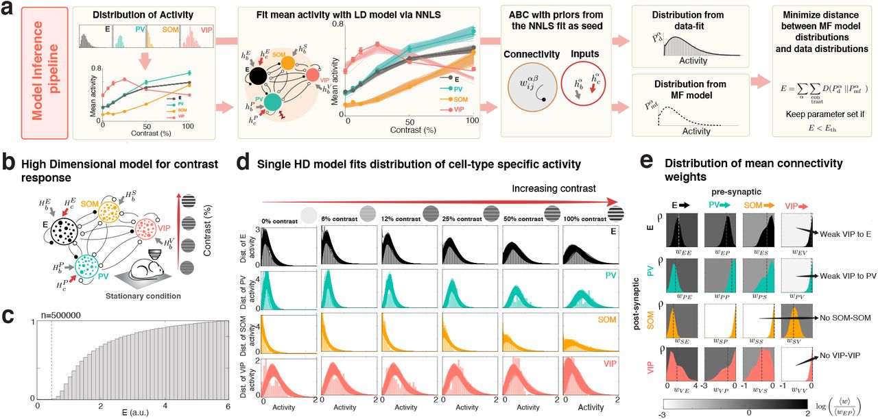
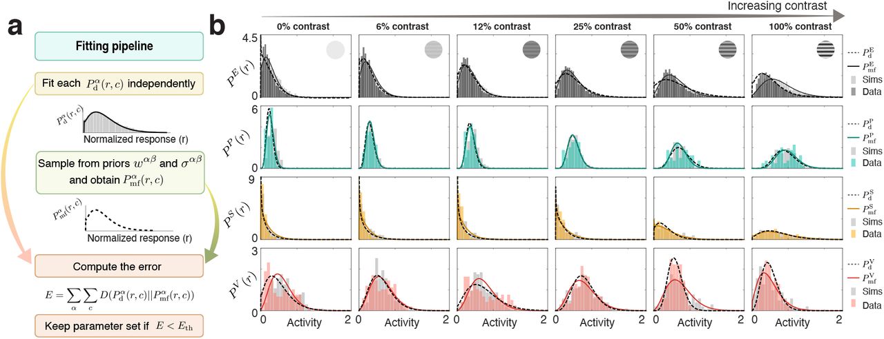
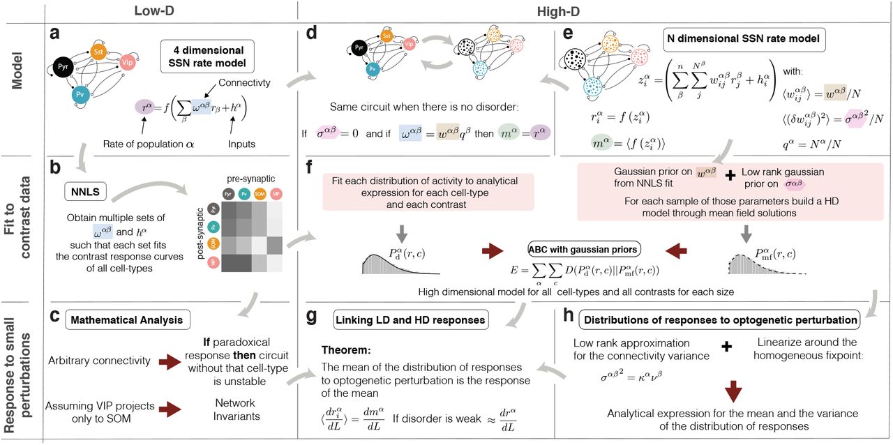
References


