

Abstract
The relative prominence of developmental bias versus natural selection is a long standing controversy in evolutionary biology. Here we demonstrate quantitatively that developmental bias is the primary explanation for the occupation of the morphospace of RNA secondary structure (SS) shapes. By using the RNAshapes method to define coarse-grained SS classes, we can directly measure the frequencies that non-coding RNA SS shapes appear in nature. Our main findings are, firstly, that only the most frequent structures appear in nature: The vast majority of possible structures in the morphospace have not yet been explored. Secondly, and perhaps more surprisingly, these frequencies are accurately predicted by the likelihood that structures appear upon uniform random sampling of sequences. The ultimate cause of these patterns is not natural selection, but rather strong phenotype bias in the RNA genotype-phenotype (GP) map, a type of developmental bias that tightly constrains evolutionary dynamics to only act within a reduced subset of structures which are easy to “find”.
Darwinian evolution proceeds in two separate steps. First, random changes to the genotypes can lead to new heritable phenotypic variation in a population. Next, natural selection ensures that variation with higher fitness is more likely to dominate the population over time. Much of evolutionary theory has focussed on this second step. By contrast, the study of variation has been relatively under-developed [1–12]. If variation is unstructured, or isotropic, then this lacuna would be unproblematic. As expressed by Stephen J. Gould, who was criticising this implicit assumption [3]:
Under these provisos, variation becomes raw material only – an isotropic sphere of potential about the modal form of a species … [only] natural selection … can manufacture substantial, directional change.
In other words, with isotropic variation, evolutionary trends should primarily be rationalised in terms of natural selection. If, on the other hand, there are strong anisotropic developmental biases, then structure in the arrival of variation may well play an explanatory role in understanding a biological phenomenon we observe today. The question of how to weight these different processes is complex (see [8, 10, 13] for some contrasting perspectives). While the discussion has moved on significantly from the days of Gould’s critique, primarily due to the growth of the field of evo-devo [7], these issues are far from being settled [5–12]
Unravelling whether a long-term evolutionary trend in the past was primarily caused by the pressures of natural selection, or instead by biased variation is not straightforward. It often means answering counterfactual questions [14] such as: What kind of variation could have occurred but didn’t due to bias? An important analysis tool for such questions was pioneered by Raup [15] who plotted three key characteristics of coiled snail shell shapes in a diagram called a morphospace [16], and then showed that only a relatively small fraction of all possible shapes were realised in nature. Indeed, developmental bias could be one possible cause of such an absence of certain forms [12]. However, it can be hard to distinguish this explanation from natural selection disfavouring certain characteristics, or else from contingency, where the evolutionary process started at a particular point but where there has simply not been enough time to explore the full morphospace.
One way forward is to study genotype-phenotype (GP) maps that are sufficiently tractable to provide access to the full spectrum of possible variation [14, 17, 18]. In this paper, we follow this strategy. In particular, we focus on the well understood GP mapping from RNA sequences to secondary structures (SS), and study how non-coding RNA (ncRNA) populate the morphospace of all possible RNA SS shapes.
RNA is a versatile molecule. Made of a sequence of 4 different nucleotides (AUCG) it can both encode information as messenger RNA (mRNA), or play myriad functional roles as ncRNA [19]. This ability to take a dual role, both informational and functional, has made it a leading candidate for the origin of life [20]. The number of functional ncRNA types found in biology has grown rapidly over the last few decades, driven in part by projects such as ENCODE [21, 22]. Well known examples include transfer RNA (tRNA), catalysts (ribozymes), structural RNA – most famously rRNA in the ribosome, and RNAs that mediate gene regulation such as micro RNAs (miRNA) and riboswitches. The function of ncRNA is intimately linked to the three-dimensional (3D) structure that the linear RNA strand folds into. While much effort has gone into the sequence to 3D structure problem for RNA, it has proven, much like the protein folding problem, to be stubbornly recalcitrant to efficient solution [23–25]. By contrast, a simpler challenge, predicting the RNA SS which describes the bonding pattern of a folded RNA, and which is therefore a major determinant of tertiary structure, is much easier to solve [26–30]. The combination of computational efficiency and accuracy has made RNA SS a popular model for studying basic principles of evolution [27, 28, 31–44].
An important driver of the growing interest in GP maps is that they allow us to open up the black box of variation – to explain, via a stripped down version of the process of development, how changes in genotypes are translated into changes in phenotypes. Unfortunately, it remains much harder to establish how the patterns typically observed in studies of GP maps [17, 18] translate into evolutionary outcomes, because natural selection must then also be taken into account. For GP maps, this means attaching fitness values to phenotypes which is difficult because fitness is hard to measure and is of course dependent on the environment, and so fluctuates.
One way forward is to simply ignore fitness differences, and to compare patterns in nature directly to patterns in the arrival of phenotypic variation generated by uniform random sampling of genotypes, which is also known as ‘genotype sampling’, or G-sampling [41]. For example, Smit et al. [34] followed this strategy and found that G-sampling leads to almost identical nucleotide composition distributions for SS motifs such as stems, loops, and bulges as found for naturally occuring structural rRNA. In a similar vein, Jörg et al. [36] calculated the neutral set size (NSS), defined as the number of sequences that fold to a particular structure, using a Monte-Carlo based sampling technique. For the length-range they could study (L = 30 to L = 50), they found that natural ncRNA from the fRNAdb database [45] had much larger than average NSS. More recently, Dingle et al. [41] developed a method that makes it possible to calculate the NSS, as well as the distributions of a number of other structural properties, for a much wider range of lengths. They found, for lengths ranging from L = 20 up to L = 126, that the distribution of NSS sizes of natural ncRNA – calculated by taking the sequences found in the fRNAdb, folding them to find their respective SS, and then working out its NSS using the estimator from [36] – was remarkably similar to the distribution found upon G-sampling. A similar close agreement upon G-sampling was found for several structural elements, such as the distribution of the number of helices, and also for the distribution of the mutational robustness.
An alternative method is to use uniform random sampling of phenotypes, so called P-sampling. If all phenotypes are equally likely to occur under G-sampling, then its out-comes will be similar to P-sampling. If, however, there is a bias towards certain phenotypes under G-sampling, an effect we will call phenotype bias, then the two sampling methods will lead to different results. When the authors of [41] calculated the distributions of structural properties such as the number of stems or the mutational robustness under P-sampling, they found large differences compared to natural RNA in the fRNAdb. The fact that G-sampling yields distributions close to those found for natural ncRNA, whereas P-sampling does not, suggests that bias in the arrival of variation is strongly affecting evolutionary outcomes in nature. As illustrated schematically in Figure 1(a), such a bias towards shapes that appear frequently as potential variation can lead to natural RNA SS taking up only a small fraction of the total morphospace of possible RNA shapes. Here we treat the morphospace more abstractly, but his pattern would carry through with more traditional morphospaces [15, 16] that utilize specific axes to describe phenotypic characteristics or RNA.

(a) Conceptual diagram of the RNA SS shape morphospace: The set of all potentially functional RNA is a subset of all possible shapes. In this paper we show that natural RNA SS shapes only occupy a tiny fraction of the morphospace of all possible functional RNA SS shapes because of a strong phenotype bias which means that only highly probable shapes are likely to appear as potential variation. We quantitatively predict the identity and frequencies of the natural RNA shapes by randomly sampling sequences for the RNA SS GP map. (b) RNA coarse-grained shapes: An illustration of the dot-bracket representation and 5 levels of more coarse-grained abstracted shapes for the 5.8s rRNA (length L = 126), a ncRNA. Level 1 abstraction describes the nesting pattern for all loop types and all unpaired regions; Level 2 corresponds to the nesting pattern for all loop types and unpaired regions in external loop and multiloop; Level 3 is the nesting pattern for all loop types, but no unpaired regions. Level 4 is the helix nesting pattern and unpaired regions in external loop and multiloop, and Level 5 is the helix nesting pattern and no unpaired regions.
Nevertheless, the evidence presented so far for this picture of a strong bias in the arrival of variation has only been for distributions over SS structures because individual SS typically only appear once in the fRNAdb. Moreover, the measurements have often been indirect, in that they used theoretical estimates for the NSS of individual sequences in the ncRNA databases. To conclusively address big questions related to the role of bias in evolutionary outcomes, a more direct measure is needed.
To achieve this goal of directly measuring frequencies, we first note that any tiny change to the bonding pattern of a full SS – illustrated by the dot-bracket notation in Figure 1(b) – means a new SS. In practice, however, many small differences are often found in homologues, suggesting that these are not critical to function. To capture this intuition that larger scale ‘shape’ is more important than some of the finer features captured by the full dot-bracket notation, Giegerich et al. [46] defined a 5-level hierarchical abstract representation of SS. At each nested level of description, the SS shape is more coarse-grained, as illustrated in Fig 1(b). By grouping together shapes with similar features, frequencies fp of ncRNA shapes can be directly measured from the fRNAdb [45]. In this paper, we show that the the frequency fp with which abstract shapes are found in the fRNAdb is accurately predicted by frequencies  that they are found for G-sampling, for lengths L = 40 to L = 126. We then discuss what these results mean in light of the longstanding controversies about developmental bias.
RESULTS
Nature only uses high frequency shapes, which are easily found
We computationally generated random RNA sequences for lengths L = 40, 55, 70, 85, 100, 126, and then folded them to their SS using the Vienna package [30], which is thought to be accurate for the relatively short RNAs we study here (Methods). Next we use the RNA abstract shapes method [46, 47] (See Figure 1(b)), to classify the folded SS into separate abstract structures. Similarly, we also took natural ncRNA sequences from the fRNAdb database [45], folded these and used the RNA abstract shape method to assign structures to them (see Methods). To compare the G-sampled RNA structures to the natural structures, a balance must be struck between being detailed enough to capture important structural aspects, but not too detailed such that for a given dataset very few repeated shapes are found, making it impossible to obtain reliable frequency/probability values. Considering our data sets, we use level 3 for all RNA of length L = 40 and L = 55 and level 5 for L 70 However, in Figures (S1) and (S2) of the SI we include all 5 other levels for L = 55, finding essentially the same results. In Figure (S3) shows all the shapes found at level 3 for L = 55.
Figure (2) shows the shape frequencies  found by Gsampling, ranked from most frequent to least frequent (blue dots). The frequency, or equivalently the NSS of these structures, vary by many orders of magnitude. The shapes which also appear in the fRNAdb database have been highlighted (yellow circles). Natural ncRNA are all within a small subset of the most frequent structures. Interestingly, a remarkably small number of random sequences, on the order of 103-105 independent random samples, is enough to find all shapes at these levels of abstraction found in the fRNAdb database [45].

The frequency  (blue dots) of each abstract shape, calculated by random sampling of sequences (G-sampling), is plotted versus the rank. Yellow circles highlight which of the randomly generated shapes were also found in the fRNAdb. Panels (a)—(f) are for L = 40, 55, 70, 85, 100, 126, respectively. The number of natural shapes are 13, 28, 9, 13, 16, and 25 in order of ascending length, while the numbers of possible shapes in the full morphospace are many orders of magnitude larger, ranging from ≈ 104 possible level 3 shapes for L = 40 to ≈ 1012 level 5 shapes for L = 126. The shapes in nature are all from a tiny set of all possible structures that have the highest
  or equivalently the highest NSS. All natural shapes found in the fRNAdb appear upon relatively modest amounts of random sampling of sequences.
To further quantify just how small a subset of the total morphospace has been explored by nature, we use analytic estimates of the total set of possible structures from [48]. These predict  for level 3 and
  for level 5, where we have taken results pertaining to minimum hairpin length of 3, and min ladder length of 1 (which is consistent with the options we used in the Vienna folding package). From these equations we estimate
  ,
,  ,
,  ,
,  ,
,  , and
, and  . By contrast, in the fRNAdb we find, at level 3, 13 structures for L = 40 and 28 for L = 55. At level 5 we find 9, 13, 16, and 25 independent structures for L = 70, 85, 100 and 126 respectively. Clearly the structures employed by natural ncRNA take up only a minuscule fraction of the whole morphospace of possible structures; the relative fraction explored decreases rapidly with increasing length.
Frequencies of shapes in nature can be predicted from random sampling
Figure (3) demonstrates that the G-sampled frequency of shapes correlates closely with the natural frequency of shapes, for a variety of lengths. In SI. A we show for L = 55 that similar results are found for different levels of shape abstraction, so that this result is not dependent on the level of coarse-graining.
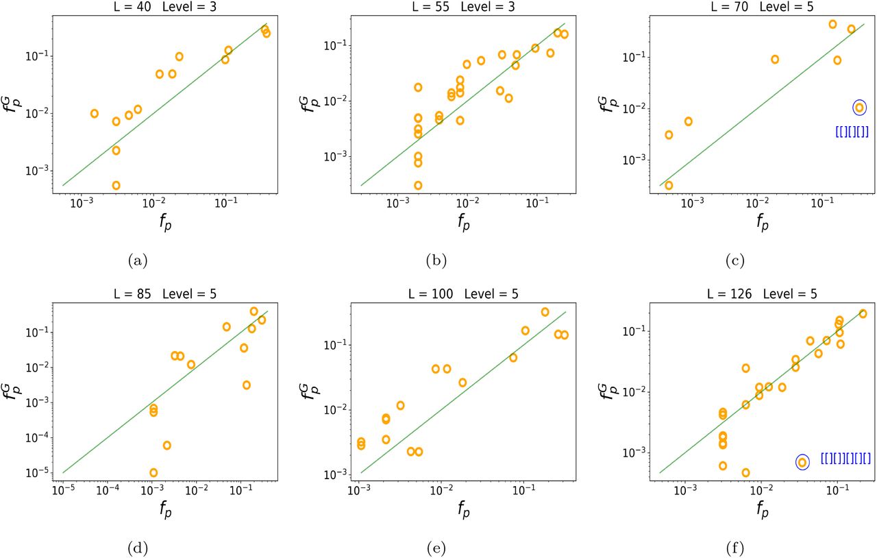
Yellow circles denote the frequencies fp of natural RNA from the fRNAdb [45]. The green line denotes x = y, i.e natural and sampled frequencies coincide. The frequency upon G-sampling  correlates well with fp: the correlation of log frequencies is: (a) L=40 Pearson r = 0.87, p-value ≈ 10−4; (b) L=55 r=0.83, p-value ≈ 10−7; (c) L=70 r =0.80, p-value ≈ 10−2; (d) L=85 r =0.78, p-value ≈ 10−3; (e) L=100 r =0.91, p-value ≈ 10−6; (f) L=126 r =0.83, p-value ≈ 10−7. We also highlight in blue two structures, namely t-RNA for L = 70 and the 5.8S ribosomal rRNA for L = 126 which have been the subject of extra scientific interest, and so are over-represented in the fRNAdb database.
We note that there is an important assumption in our interpretation, which is that the frequency with which structures are found in the fRNAdb is similar to the frequency with which they are found in nature. To first order it is reasonable to assume that this is true, as the databases are typically populated by finding sequences that are conserved in genomes, a process that should not be too highly biased. In addition, the good correlation between the  and fp found here provides additional a posteriori evidence for this assumption as it would be hard to imagine how this close agreement could hold if there were strong man-made biases in the database. Nevertheless, there are structures that have been the subject of greater researcher interest, and one may expect them to be deposited in the database with higher frequency. We give two examples in Figure (3)(c) and (f) of outliers that are over-represented (with high confidence) compared to our prediction. They are the shape [[][][]], which includes the classic clover leaf shape of transfer RNA, and [[][]][][][] which corresponds to the 5.8S ribosomal RNA (rRNA, as shown in Figure 1b) which has also been studied extensively. In SI B we show that pruning the data does not change the correlations. Finally, note that our assumption that the frequency of shapes in nature is similar to the frequency of shapes in the database is not required for our previous finding that nature only uses high frequency shapes. That observation stands, whether or not the database frequencies are close to natural frequencies. Further, for one length (L = 100) we show in SI. C that qualitatively similar rank and correlation plots (Figure S5) appear using a different database, the popular Rfam [49, 50], where structures are determined not by folding, but by a consensus alignment procedure. Hence our main findings are unlikely to be due to database biases.

Rank plot for L = 55, across all abstraction levels 1, 2, 3, 4 and 5, with 5×10⁶ random samples for each level, compared to the natural frequencies from the fRNAdb. The number of random shapes and number of natural shapes (in brackets) found for levels 1—5 are 20587 (203), 4268 (113), 183 (28), 139 (23), and 16 (5).

The frequency of shapes in a database correlates with the frequency in nature for L = 55, across all abstraction levels 1, 2, 3, 4 and 5, with 5×10⁶ random samples for each level. For lower abstraction levels, there are fewer samples per shape, and hence more noise. With higher levels and hence more samples per shape, there are less points, but also less noise and a clearer correlation. The green line is simply x = y; it is not a fit to the data.

Shape array for L = 55 RNA at level 3, showing the 183 shapes found by sampling 5 ×10⁶ random sequences, in order of their rank by frequency  . The 28 naturally occurring shapes from the fRNAdb are highlighted in yellow, demonstrating that only a small fraction of the total morphospace of shapes is occupied by RNAs found in nature, and that these are all highly frequent structures. We estimate that there are on the order of 107 possible level 3 structures for L = 55 RNA, so that this array only shows a tiny fraction of the total.

Frequency plots for natural and random data, after excluding RNA labelled “putative”. (a) L = 55, r = 0.77, p-value ≈ 10−5 (219 sequences remain after exclusions, 24 shapes); (b) L = 70 excluding RNA labelled ‘putative’, and tRNA. The correlation is r = 0.98, p-value ≈ 10−4 (518 sequences remain after exclusions, 7 shapes); (c) and L = 126, r =0.74, p-value ≈ 10−4 (184 sequences remain after exclusions, 23 shapes).

Rank and correlation plots for natural and random data, using Rfam data. (a) Combined data for L = 95, 96, …, 104, 105 natural consensus structures rank plot; and (b) L = 95 to 105, correlation plot with r = 0.96, p-value ≈ 10−6. The data contains 4124 sequences, which yielded 13 unique shapes (level 5). Sampling 105 random sequences found 12 out of the 13 unique natural shapes.
DISCUSSION
We first recapitulate our main results below under three headings, and discuss their implications for evolutionary theory.
(A) Nature only utilizes a tiny fraction of the RNA SS phenotypic variation that is potentially available
Besides being an interesting fact about biology, this result has implication for synthetic biology as well. There is a vast morphospace [16] of structures that nature has not yet sampled. If these could be artificially created, then they could be mined for new and potentially intriguing functions.
(B) Remarkably small numbers of sequences are needed to recover the full set of abstract shapes in the fRNAdb database
This effect is enhanced by the fact that we have coarse-grained the SS to allow for direct comparisons. As shown in the SI section A, for finer descriptions of the SS, more sequences are needed to obtain all natural structures, but the numbers remain modest.
To calibrate just how remarkably small these numbers of sequences needed to produce the full spectrum of structures found in nature are, consider that the total number of sequences NG grows exponentially with length as NG = 4L. This scaling implies unimaginably vast numbers of possible sequences, even for modest RNA lengths. For example, all individual sequences of length L = 77 together would weigh more than the earth, while the mass of all combinations of length L = 126 would exceed that of the observable universe [14]. Such hyper-astronomically large numbers have been used to argue against the possibility of evolution producing viable phenotypes, based on the claim that the space is too vast to search through. See the Salisbury-Maynard Smith controversy [51, 52] for an iconic example of this trope. And it is not just evolutionary skeptics who have made such claims. In an influential essay, Francois Jacob wrote [53]:
The probability that a functional protein would appear de novo by random association of amino acids is practically zero.
A similar argument could be made for RNA. Our results suggest instead that a surprisingly small number of random sequences are sufficient to generate the basic RNA structures that are sufficient for life in all its diversity. This finding is relevant for the RNA world hypothesis [20], since it suggests that relatively small numbers of sequences are needed to facilitate primitive life. In the same vein, it helps explain why random RNAs can already have a remarkable amount of function [54], similarly to what is suggested for proteins in the rapidly developing field of de novo gene birth [55–58].
(C) The frequency with which structures are found in nature is remarkably well predicted by simple G-sampling
This result is perhaps the most surprising of the three because these G-sampling ignores natural selection. It is widely thought that structure plays an important part in biological function, and so should be under selection.
The key to understanding results (A)–(C) above can be found in one of the most striking properties of the RNA SS GP map, namely strong phenotype bias which manifests in the enormous differences in the G-sampled frequencies (or equivalently the NSS) of the SS [27]. For example, for L = 20 RNA, the largest system for which exhaustive enumeration was performed [39], the difference in the  between the most frequent SS phenotype and the least frequent SS phenotype was found to be 10 orders of magnitude. For L = 100 this difference was estimated to be over over 50 orders of magnitude [41]. Such phenotype bias also explains why G-sampling and P-sampling are so different [41]: a small fraction of high frequency phenotypes take up the majority of the genotypes, and thus dominate under G-sampling.
Evolutionary modelling that takes strong bias in the arrival of variation into account is rare. Population-genetic models that do include new mutations typically consider a genotype-to-fitness map, which often includes an implicit assumption that all phenotypes are equally likely to appear as potential variation, something akin to P-sampling. A notable exception is work by Yampolsky and Stoltzfus [59] which has been applied, for example, to the effect of mutational biases [60, 61].
For the specific case of RNA, however, the effect of strong phenotype bias was treated explicitly in ref [39], where it was shown that for the RNA SS GP map, the mean rate ϕpq at which new variation p appears in a population made up of phenotype q can be quite accurately approximated as  , where ρq is the mean mutational robustness of genotypes mapping to q. This simple relationship holds for both low and high mutation rates. In other words, the local rate at which variation appears closely tracks the global frequency
  of the different potential phenotypes, which is exactly what G-sampling measures.
While it is not so controversial that biases could affect outcomes under neutral mutation, see e.g. [62], the strongest disagreements in the field centre around the effect of bias in adaptive mutations [5–13, 60, 61]. Since RNA structure is thought to be adaptive, the main question to answer is how phenotype bias affects RNA evolution when natural selection is also at work. In ref [39], the authors explicitly treat cases where phenotype bias and fitness effects interact. They provide calculations of an effect called the arrival of the frequent, where the enormous differences in the rate at which variation arrives implies that frequent phenotypes are likely to fix, even if other higher fitness, but much lower frequency phenotypes are possible in principle. This same effect has also been observed in evolutionary modelling of gene regulatory networks [63]. To avoid confusion, we note that the arrival of the frequent is fundamentally different from the survival of the flattest [64], which is a steady-state effect. There, two phenotypes compete, and at high mutation rates, the one with the largest neutral set size can dominate in a population, even if its fitness is smaller. By contrast, the arrival of the frequent is a non-ergodic effect in the sense that it is not about a steady state with competing phenotypes in a population. Instead, it is about what appears in the first place. Indeed, it can be shown that for strong bias [39] that to first order, the number of generations Tp at which variation on average first appears in a population scales as  in both the high and the low mutation regimes. Since
  varies over many orders of magnitude, on a typical evolutionary time-scale T, only a limited amount of variation (typically that with Tp ≲ T) can appear. Variation can only fix if it appears in a population. Thus, natural selection acts on SS variation that has been pre-sculpted by the GP map [41].
The close agreement between G-sampling frequencies and measured frequencies of natural ncRNA suggests that once an SS is found that is good enough, natural selection mainly works by further refining parts of the sequence for function, rather than significantly altering the structures. Thus the arrival of the frequent picture, which is fundamentally about strongly anisotropic variation, provides a mechanism that rationalises all three main classes of observations above.
There is a profound connection between the arrival of the frequent effect in evolution, and the dynamics of optimisation in deep neural networks (DNNs). Just as was found for the RNA GP maps, the mapping from parameters to DNN functions can be hugely biased [65, 66]. DNNs are often optimised with stochastic gradient descent (SGD) [67] which follows the contours of a complex loss-landscape, much as evolution follows a fitness-landscape over time. Given the extremely strong bias, functions with a large volume of parameters mapping to them are, in close analogy to the arrival of the frequent phenomenon described above, much more likely to appear in a search process through the space of parameters, even if there are other functions with similar or potentially even better loss values. It was recently shown [68] that the probability that SGD converges on a particular function can be remarkably well approximated by the (Bayesian) probability that this function obtains upon random sampling of DNN parameters, which is directly analogous to G-sampling. This phenomenology was observed for multiple data sets and loss functions, suggesting that a mechanism much like the arrival of the frequent works quite robustly for these highly biased systems also, strengthening our hypothesis that this mechanism can hold across multiple evolutionary scenarios for highly biased GP maps.
It is interesting to consider whether our arguments that strong phenotype bias affects adaptive evolution can shed light on a related controversy around mutational biases. For example Stoltzfus and McCandlish [60], argued that transition-transversion mutation bias in the arrival of mutations can affect the frequency of adaptive amino acid substitutions. This conclusion was criticised by Svensson and Berger [13], who argue that the bias may not be large enough to overcome fitness differences, and that there may be alternative adaptive arguments for the codon substitution patterns observed in [60]. The basic arguments behind mutational biases having an effect in adaptive evolution are similar in spirit to our arguments for phenotype bias, but there are also differences. Phenotype bias is about the rate at which phenotypes arise, and here we treat all mutations as being equally likely, while mutational bias captures inhomogeneities in the rate at which mutations arise along a genome. Mutation bias is also typically much smaller than phenotype bias, and so its effects should only be noticeable mutation limited regimes. The global differences in  for the whole morphospace are enormous, but they are on the order of just a few orders of magnitude for those structures found in nature. While overall these differences are larger than typical mutational biases, the good correlation between fp and
  provides indirect evidence in favour of the more modestly strong mutational bias affecting adaptive evolution as well.
The picture of strong phenotype bias is also consistent with SELEX experiments [69, 70], where artificial selection for RNA function can lead, with a relatively small amount of material, to the repeated convergent evolution of the same structures. Famous examples include RNA aptamers [71, 72] and the hammerhead ribozyme [73], which also shows convergence in nature [58]. In light of the unimaginably small fraction of the hyper-astronomically large numbers of possible sequences these experiments explore, this convergent evolution seems highly surprising. But when we consider the strong phenotype bias in the RNA sequence to structure mapping, then a possible explanation emerges. SELEX experiments rely on artificial selection to refine sequences and hone in on a particular function. While natural selection is the ultimate reason why a particular function emerges (such as self-cleaving catalytic activity for the hammerhead ribozyme), we hypothesise that the same structures emerge (after all, multiple structures could, in principle, produce the same function) because of phenotype bias. In other words, to use Mayr’s famous distinction [74–76], for RNA SS, phenotype bias is the ultimate, and not merely the proximate cause of the evolutionary convergence of the structures found in SELEX experiments and in nature. The general idea that developmental biases could help explain convergence is not new [1, 77, 78], but we believe that the type of phenotype bias we are proposing here is new to the literature on evolutionary convergence.
How is phenotype bias related to the broader literature on developmental bias? On the one hand phenotype bias acts as a constraint [1], in that it limits what kind of variation natural selection can work on. Whether it also acts as a developmental drive [79] that facilitates adaptive evolution would hinge on there being advantages to the kinds of structures that it favours. For RNA, G-sampled structures are on average different from P-sampled structures, for example they have higher mutational robustness, and fewer stems [41], and so there is bias towards these characteristics, which may be adaptive.
Where phenotype bias differs the most from classic examples of developmental bias such as the universal pentadactyl nature of tetrapod limbs, is that the latter are thought to occur because evolution took a particular turn in the past that locked in a developmental pathway, most likely through shared ancestral regulatory processes [80]. If one were to rerun the tape of life again, then it is conceivable that a different number of digits would be the norm. By contrast phenotype bias predicts that the same spectrum of RNA shapes would appear, populating the morphospace in the same way. It is true that given enough time, a larger set of RNA shapes could appear, but the exponential nature of the bias implies that orders of magnitude more time are needed to see linear increases in the number of available shapes.
It is also interesting to compare phenotype bias to adaptive constraints. For example, there are many scaling laws such as Kleiber’s law which states that the metabolic rate of organisms scales as their mass to the 3/4 power. This has been shown to hold over a remarkable 27 orders of magnitude [81]! The morphospace of metabolic rates and masses is therefore highly constrained. Such scaling laws can be understood in an adaptive framework from the interaction between various basic physical constraints [81], rather than from biases in the arrival of variation. Phenotype bias also arises from a fundamental physical process [82] and limits the occupation of the RNA morphospace. But it is, by contrast, a non-adaptive explanation. It may be closest in spirit to some constraints that are postulated in biological or process structuralism [83], but here the constraint arises from the GP map itself.
Finally, the fact that G-sampling does such a good job at predicting the likelihood that SS structures are found in nature also has implications for the study of selective processes in RNA structure [84, 85]. We propose here that signatures of natural selection should be measured by considering deviations from the null-model provided by Gsampling.
In conclusion, while the RNA sequence to SS map describes a pared down case of development, this simplicity is also a strength. It allows us to explore counterfactual questions such as what kind of physically possible phenotypic variation did not appear due to phenotypic bias. This system thus provides the cleanest evidence yet for developmental bias strongly affecting evolutionary outcomes. Many other GP maps show strong phenotype bias [17, 18, 82]. An important question for future work will be whether there is a universal structure to this phenotype bias and whether it has such a clear effect on evolutionary outcomes in other biological systems as well.
MATERIALS AND METHODS
Folding RNA
We use the popular Vienna package [28, 30], to fold sequences to structures, with all parameters set to their default values (e.g. the temperature T = 37°C). This method is thought to be especially accurate for shorter RNA. The numbers of random samples were 5 × 10⁶ for L = 40 and L = 55, and 105 for L = 70, 85, 100, 126. For G-sampling, we choose random sequences, and fold each one. Sequences from the fRNAdb database[45] were folded using the Vienna package with the same parameters as above.
Abstract shapes
RNA SS can be abstracted in standard dot-bracket notation, where brackets denote bonds, and dots denote unbonded pairs. To obtain coarse-grained abstract shapes [47] of differing levels we used the RNAshapes tool available at https://bibiserv.cebitec.uni-bielefeld.de/rnashapes. The option to allow single bonded pairs was selected, to accommodate the Vienna folded structures which can contain these.
Natural fRNAdb sequences
For each length, we took all available natural non-coding RNA sequences from the fRNAdb database [45] and discarded a very small fraction of sequences because they contained non-standard letters such as ‘N’ or ‘R’. The numbers of natural sequences used were:
(L=40) 659 sequences, yielding 13 unique shapes at level 3;
(L=55) 507 sequences, yielding 28 unique shapes at level 3;
(L=70) 2275 sequences, yielding 18 unique shapes at level 5;
(L=85) 913 sequences, yielding 13 unique shapes at level 5;
(L=100) 932 sequences, yielding 16 unique shapes at level 5;
(L=126) 318 sequences, yielding 25 unique shapes at level 5.
Author Contributions
KD and AAL conceived the project. KD and FG performed the sampling of the databases, and the calculations of the RNA SS. KD, PS and AAL analysed the data and wrote the manuscript.
Competing Interests
None.
SUPPLEMENTARY INFORMATION
A. L = 55 data for levels 1 to 5
In Figures (S1) and (S2) we show plots for the L = 55 data using all five coarse-grained abstraction levels of RNAshapes from Giegerich et al. [46]. These figures demonstrate very similar results to those found in the main text for level 3. This qualitative agreement strongly suggests that our main findings are robust to our choice of level. Note that the lowest possible frequencies directly measured in the database are limited by the relatively small number of samples, which affects lower levels of coarse-graining more strongly, because there are more such shapes available. The rank plots in Figure (S1) suggest that as more sequences are added, a wider range of frequencies will be found, improving the correlation at low frequency in Figure (S2). Finally, for level 3, we list all the shapes in Fig. S3 to help illustrate the occupation of the RNA shape morphospace. Similar plots could be made for other levels of abstraction.
B. Excluding putative sequences
Some sequences in the fRNAdb are labelled as putative, meaning that they are identified as potentially functional (due, for example, to conservation), but that the exact function of the RNA is currently unknown. To check that these putative RNA are not mainly responsible for the high correlations between the frequency in the database, fp, and the frequency upon G-sampling,  , we make, for a few lengths, the same correlation plots as in the main text but after excluding sequences labeled putative.
Figure (S4) shows the scatter plots for L = 55, L = 70 and L = 126, after excluding these putative RNA. For L = 70, all tRNA have also been removed, because for this length the majority of sequences are tRNA, and hence the dataset is somewhat unusual. As is apparent from the figure, the correlations observed in the main text are not sensitive to the removal of these putative structures.
C. L ≈ 100 data from Rfam
To briefly check that our results maintain for a different database, and with secondary structures not obtained via computationally predicted algorithms, here we study data from the Rfam [49, 50] database.
All RNAs of length 95 to 105 were taken from all available seed sequences of ncRNA families from the Rfam database. Their secondary structures were obtained by aligning to the consensus structure of the seed alignment for respective RNA families. Note that this is different to analysis we performed for the main text, where instead secondary structures were predicted via folding algorithms, using the popular Vienna package.
The total number of sequences obtained were 4309, but a small fraction (ie 185 or 4.3%) of these were discarded because they were invalid secondary structures according to the folding rules used by the shape abstracter. For example, some of the consensus structures contained motifs with a loop of length 1, ie (.), which are deemed invalid. The reason we combined data for lengths 95 to 105 (rather than just using L = 100) is that there were relatively few sequences and RNA shapes for just L = 100, and so by combining data from other lengths close to 100, we obtain better statistics.
Qualitatively similar rank and correlation plots appear when using Rfam data for L ≈ 100 in Figure S5 as compared to the correlation plots in the main text. Hence we see that our correlations findings are not artefacts of either the database which we have used, nor the method for obtaining secondary structures.
Acknowledgements
We thank David McCandlish for helpful discussions.
References
- [1].↵
- [2].
- [3].↵
- [4].
- [5].↵
- [6].
- [7].↵
- [8].↵
- [9].
- [10].↵
- [11].
- [12].↵
- [13].↵
- [14].↵
- [15].↵
- [16].↵
- [17].↵
- [18].↵
- [19].↵
- [20].↵
- [21].↵
- [22].↵
- [23].↵
- [24].
- [25].↵
- [26].↵
- [27].↵
- [28].↵
- [29].
- [30].↵
- [31].↵
- [32].
- [33].
- [34].↵
- [35].
- [36].↵
- [37].
- [38].
- [39].↵
- [40].
- [41].↵
- [42].
- [43].
- [44].↵
- [45].↵
- [46].↵
- [47].↵
- [48].↵
- [49].↵
- [50].↵
- [51].↵
- [52].↵
- [53].↵
- [54].↵
- [55].↵
- [56].
- [57].
- [58].↵
- [59].↵
- [60].↵
- [61].↵
- [62].↵
- [63].↵
- [64].↵
- [65].↵
- [66].↵
- [67].↵
- [68].↵
- [69].↵
- [70].↵
- [71].↵
- [72].↵
- [73].↵
- [74].↵
- [75].
- [76].↵
- [77].↵
- [78].↵
- [79].↵
- [80].↵
- [81].↵
- [82].↵
- [83].↵
- [84].↵
- [85].↵


