

1. Abstract
Genome-wide association studies (GWAS) have identified thousands of genetic variants that are associated with complex traits. However, a stringent significance threshold is required to identify robust genetic associations. Leveraging relevant auxiliary data has the potential to boost statistical power to exceed the significance threshold. Particularly, abundant pleiotropy and the non-random distribution of SNPs across various functional categories suggests that leveraging GWAS test statistics from related traits and/or functional genomic data may boost GWAS discovery. While type 1 error rate control has become standard in GWAS, control of the false discovery rate (FDR) can be a more powerful approach as sample sizes increase and many associations are expected in each study. The conditional false discovery rate (cFDR) extends the standard FDR framework by conditioning on auxiliary data to call significant associations, but current implementations are restricted to auxiliary data satisfying specific parametric distributions. We relax the distributional assumptions, enabling an extension of the cFDR framework that supports auxiliary data from any continuous distribution (“Flexible cFDR”). Our method is iterative, whereby additional layers of auxiliary data can be leveraged in turn. Through simulations we show that flexible cFDR increases sensitivity whilst controlling FDR after one or several iterations. We further demonstrate its practical potential through application to an asthma GWAS, leveraging various functional data to find additional genetic associations for asthma, which we validated in the larger UK Biobank data resource.
2. Introduction
Genome-wide association studies (GWAS) identify risk loci for a phenotype by assaying single nucleotide polymorphisms (SNPs) in large participant cohorts and marginally testing for associations between each SNP and the phenotype of interest. Conducting univariate tests for each SNP in parallel presents a huge multiple testing problem for which a stringent p-value threshold is required to confidently call significant associations.
The statistical power to detect associations can be increased by leveraging relevant auxiliary covariates. For example, pervasive pleiotropy throughout the genome1 suggests that leveraging GWAS test statistics for related traits may be beneficial, whilst the non-random distribution of trait-associated SNPs across various functional categories2 suggests that incorporating functional genomic data may also be useful. In fact, the expansive range of relevant auxiliary covariates has accumulated in a wealth of methods that have been developed for the general purpose of leveraging auxiliary covariates (typically SNP-level data) with test statistics for variables (typically GWAS p-values for SNPs) to improve statistical power for GWAS discovery.
The simplest approach is “independent filtering” 3 whereby test statistics are first censored based on the value at the covariate and a type-1 error controlling procedure (for example the Bejamini-Hochberg (BH) procedure4) is then applied on the remaining subset of test statistics to call significant associations. First introduced by Holm in 19795, p-value re-weighting methods (and the extension for weighted hypothesis testing by Genovese et al.6) can also be used to prioritise variables by leveraging auxiliary covariates with test statistics7–15. However, these methods generally require specification of a normalised weighting scheme and typically involve a binning step used to derive bin-specific weights that are allocated to large groups of variables8,9,14–16, meaning that the entire dynamic range of the auxiliary data may not be fully exploited.
The Bayesian framework offers an intuitive opportunity to include auxiliary covariates in the form of a prior distribution17–21. However, it is non-trivial to convert auxiliary covariate data into prior probabilities for use in the model, and the validity of inference is based on the accuracy of the parametric assumptions of the Bayesian model. Other approaches include methods that focus power on the more promising variables, for example by constructing negative controls from the data which can then be used to rank and select variables22,23.
A consistent aim of the aforementioned methods is to control for the number of false discoveries. A general criterion for discovery using test statistic-covariate data pairs is to minimise type 2 errors (false negatives) whilst controlling for type-1 errors (false positives). This criterion is applicable to GWAS discovery using covariates and has been explored extensively in the statistics literature. Optimal rejection regions for this criterion (defined on the 2-dimensional plane of test statistics and covariate values) can be derived on the basis of a ratio of bivariate probability density functions (PDFs) under the null hypothesis (no association) and the alternative hypothesis (association)24–27. Statistical methods that directly estimate this ratio have been developed25–27 but estimating PDFs is generally a hard statistical problem and the underlying parametric assumptions may not be satisfied, resulting in the loss of statistical guarantee.
Conditional false discovery rates (cFDRs) approximate the aforementioned optimal ratio using cumulative density functions (CDFs) rather than PDFs, which are generally easier to estimate accurately as many more data points contribute to most estimates. Andreassen and colleagues28–30 developed and applied the cFDR method to increase GWAS discovery (in the “principal trait”) by leveraging GWAS test statistics from a genetically related (“conditional”) trait. The cFDR is defined by the probability of the null hypothesis (no genetic association) in the principal trait, given that the p-values for the principal trait and the conditional trait are below some trait specific thresholds. Andreassen and colleagues28–30 identified significant SNPs as those with cFDR ≤ α (where typically α = 0.05 or α = 0.01), however the expected overall FDR amongst these sets of SNPs is greater than α, meaning that this method does not control FDR31. Liley and Wallace31 proposed a method to derive an upper bound for the expected FDR amongst such sets of SNPs but this method is conservative, and potentially extremely so. A less conservative approach has been recently proposed which uses the cFDR framework to generate quantities analogous to p-values that can be readily FDR controlled24.
Here, we describe “Flexible cFDR”, an extension of the cFDR framework that supports continuous auxiliary data from any arbitrary distribution, extending its use beyond only GWAS. As in the existing cFDR framework24, our method requires GWAS test statistics for the trait of interest and auxiliary SNP-level data to output quantities analogous to p-values (called “v-values”), meaning that the method can be applied iteratively to incorporate additional layers of auxiliary data. We show through detailed simulations that flexible cFDR increases sensitivity whilst controlling specificity, and performs as well or better than the existing cFDR framework in use-cases where both methods are supported. A natural utilisation of our method is to leverage relevant functional genomic data with GWAS p-values to boost statistical power for GWAS discovery. To illustrate this, we leverage a variety of functional genomic data with GWAS p-values for asthma32 to prioritise new genetic associations. We compare results to those from other GWAS signal prioritisation approaches that integrate functional data (GenoWAP17 and FINDOR8) and evaluate results according to validation status in the larger UK Biobank data set33.
3. Methods
3.1 Conditional false discovery rate
Consider p-values for m SNPs, denoted by p1, …, pm, that measure the likelihood of the data under the null hypothesis of no association between the SNP and a principal trait (denoted by  ). Let p1, …, pm be realisations from the random variable P. The false discovery rate (FDR) is defined as the probability that the null hypothesis is true for a random SNP in a set of SNPs with P ≤ p:
 Given additional p-values, q1, …, qm, for the same m SNPs for a “conditional trait”, the FDR can be extended to the conditional FDR (cFDR). Assuming that pi and qi (for i = 1, …, m) are independent and identically distributed (iid) realisations of random variables P, Q satisfying:
 then the conditional false discovery rate (cFDR) is defined as the probability
  is true at a random SNP given that the observed p-values at that SNP are less than or equal to p in the principal trait and q in the conditional trait28,29. Using Bayes theorem,
 The cFDR framework implicitly assumes that there is a non-negative correlation between p and q, meaning that SNPs with smaller p-values in the conditional trait are enriched for smaller p-values in the principal trait. This assumption is naturally satisfied in the typical use-case of cFDR that leverages p-values for genetically related traits.
Using Bayes theorem and standard conditional probability rules, Equation 3 can be simplified to31:
 It is conventional in the cFDR literature to conservatively approximate
  , and this is reasonable in the GWAS setting where the proportion of true signals is expected to be very low. Given the assumptions in Equation 2, we can also approximate
  . The estimated cFDR is therefore:
 and existing methods use empirical CDFs to estimate
  and P (P ≤ p, Q ≤ q)24,28.
3.2 Flexible cFDR
The standard cFDR derivation holds in the more general setting where q1, …, qm are real continuous values from some arbitrary distribution that is monotonic in p. However, the accuracy of empirical CDF estimates near the extremes of p and/or q may be low due to sparsity of data. This was our first motivation to extend the cFDR framework for data pairs consisting of p-values for the principal trait (p) and continuous covariates from any arbitrary distribution (q). We call our method “flexible cFDR”.
To estimate both  and P (P ≤ p, Q ≤ q) in Equation 5, we first fit a bivariate kernel density estimate (KDE) using a normal kernel with constant variance I2 to the pairs of data (p, q). We convert the p-values for the principal trait to Z-scores (Zp) and model the PDF corresponding to Zp, Q in the usual way as
 where ϕ is the standard normal density and the values σp and σq are the bandwidths determined using a well-supported rule-of-thumb34, which assumes independent samples. Consequently, we fit the KDE to a subset of independent data points in the data set (independent SNP sets can be readily found using a variety of software packages including LDAK35 and PLINK36). We sum over P and Q to estimate P (P ≤ p, Q ≤ q).
Hard thresholding is used to approximate the distribution of  by Q|P > 1/2 in the earlier cFDR methods24,28. Instead, we opt to utilise the local FDR (lFDR) framework37, which estimates
  . We approximate
  assuming that the majority of information about
  is contained in P so that
 where P (P = p, Q = q) is estimated from our bivariate KDE and
  is estimated using FDR.
From this,  is estimated by integrating over P and
  is then estimated by integrating over Q. Finally, we integrate over Q to obtain
 where we use ^ to denote that these are estimates under the assumption
  Our final cFDR estimator is therefore:

3.3. Mapping p-value-covariate pairs to v-values
Having derived  values for each p-value-covariate pair, a simple rejection rule would be to reject
  for any
 , for 0 < α < 1. However, as discussed in Liley and Wallace24,
  is not monotonically increasing with pi and we don’t want to reject the null for some (pi, qi) and not for some other pair (pj, qj) with qi = qj but pj < pi.
Andreassen et al.28 use the decision rule:
 which closely follows the B-H procedure4. Yet unlike the B-H procedure, this rejection rule does not control FDR at α 31. Liley and Wallace24 described a method to control the FDR, but it is currently only suited to instances where the auxiliary data may be modelled using a mixture of centered normal distributions (for example by transforming auxiliary p-values to Z scores;
  . This was our second motivation to extend the method to any continuously valued q, removing this restriction.
We define “L-regions” as the set of points with  and the “L-curve” as the rightmost border of the L-region24. Specifically, we calculate
  values for p, q pairs defined using a two-dimensional grid of p and q values. For each observed pi, qi pair we find the L-curve, which corresponds to the contour of estimated
  . We then define the L-region from this L-curve.
We derive v-values, defined as the probability of a newly-sampled realisation (p, q) of P, Q falling in the L-region under  . Note this definition is analogous to that of a p-value, which can then be readily FDR controlled using any FDR controlling procedure. These v-values are readily calculable by integrating the PDF of
  over the L-region24:
 where f0(p, q) is the PDF of
  . In the original method, this PDF is estimated using a mixture-Gaussian distribution, but this does not hold in the more general setting described here where the distribution of the auxiliary data is arbitrary, and therefore not necessarily able to be modelled using a mixture of centered normal distributions. We therefore utilise the assumptions in Equation 2 to estimate:
 where
where  and is therefore the PDF of the standard uniform distribution and
  is already calculated in an intermediate step when deriving
  .
.
The v-value can be interpreted as the probability that a randomly-chosen (p, q) pair has an equal or more extreme  value than
  under
under  . Our framework can therefore be applied iteratively, using the v-value from the previous iteration as the test-statistics in the current iteration24, allowing users to incorporate additional layers of auxiliary data into the analysis when they become available.
3.4. Adapting to sparse data regions
To ensure that the KDE approximated in our method constitutes a true density that attains the value 0 at the limits of its support, we define its limits to be 10% wider than the range of the data. However, this introduces a sparsity problem whereby the data required to fit the KDE in or near these regions is very sparse. Adaptive KDE methods that find larger value bandwidths for these sparser regions are computationally impractical for large GWAS data sets. Instead, we opt to use left-censoring whereby all q < qlow are set equal to qlow and the value for qlow is found by considering the number of data points required in a grid space to reliably estimate the density. Note that since our method utilises cumulative densities, the sparsity of data for extremely large q is no longer an issue.
Occasionally, in regions where (p, q) are jointly sparse, the v-value can appear extreme compared to the p-value. To avoid artifactually inflating evidence for association, we fit a spline to log10(v/p) against q and calculate the distance between each data point and the fitted spline, mapping the small number of outlying points back to the spline and recalculating the corresponding v-value as required (Figure S1).
3.5. Simulations
We used simulations to assess the performance of flexible cFDR when iteratively leveraging various types of auxiliary data. We validated flexible cFDR against the existing framework, which we call “empirical cFDR” 24, in two cases where q ∈ [0, 1] as it requires. We then evaluated the performance of cFDR in three novel use-cases where the auxiliary data is no longer restricted to [0, 1].
3.5.1. Simulating GWAS results (p)
We first simulated GWAS p-values for the “principal trait” to be used as p in our simulations. We collected haplotype data from the UK10K project38 (REL-2012-06-02) for 80,356 SNPs with MAF ≥ 0.05 residing on chromosome 22. We split the haplotype data into 24 LD blocks representing approximately independent genomic regions defined by the LD detect method39. Within each LD block, we sampled 2, 3 or 4 causal variants with log odds ratio (OR) effect sizes simulated from the standard Gaussian prior used for case-control genetic fine-mapping studies, N (0, 0.22)40 (the mean number of simulated causal variants in each simulation was 54). We then used the ‘simGWAS’ R package41 to simulate Z-scores from a GWAS in each region for 20,000 cases and 20,000 controls. We collated the Z-scores from each region and converted these to p-values representing the evidence of association between the SNPs and the arbitrary principal trait.
To generate an independent subset of SNPs required to fit the KDE, we converted the haplotype data to genotype data and used the ‘write.plink’ function in the PLINK software36 to generate the files required for the LDAK software35. We generated LDAK weights for each of the 80,356 SNPs and used the subset of 14,234 SNPs with non-zero LDAK weights as the independent subset of SNPs (an LDAK weight of zero means that its signal is (almost) perfectly captured by neighbouring SNPs)42.
3.5.2. Simulating auxiliary data (q)
We consider five use-cases of cFDR (simulations A-E), defined by (i) the distribution of the auxiliary data q (ii) the relationship between p and q and (iii) the relationship between different q in each iteration (5 realisations of q were sampled in each simulation so that cFDR could be applied iteratively) (Table 1).
Each simulation type (A-E) is defined by the distribution of q, the relationship between p and q and the relationship between the realisations of q sampled for each iteration of cFDR. Pairwise correlation values are the Pearson correlation coefficients.
In simulation A, we sampled q ∼ Unif (0, 1) to represent iterating over null p-values (Figure S2A). In simulation B, we investigated the standard use-case of cFDR by iterating over p-values from “related traits” (Figure S2B). To do this, we used the simGWAS R package41 to simulate p-values, and specified “related traits” as those that shared ≥ 20 of the causal variants with the principal trait or those that shared slightly fewer causal variants but had p-values that were highly correlated with those for the principal trait (r > 0.15).
In simulations C-E, we simulated auxiliary data that was no longer restricted to [0, 1]. In simulation C, we sampled q from a bimodal mixture normal distribution that was independent of p: q ∼ 0.5×N (−2, 0.52)+0.5×N (3, 22) (Figure S2C). In simulations D and E we simulated continuous auxiliary data that was dependent on p by first defining “functional SNPs” as causal variants plus any SNPs within 10,000 bp, and “non-functional SNPs” as the remainder. In simulation D, we then sampled q from different mixture normal distributions for functional and non-functional SNPs:
 where µ1 ∈ {2.5, 3, 4}, µ2 ∈ {−1.5, −2, −3}, w ∈ {0.6, 0.7, 0.8, 0.9, 0.95} vary across iterations.
Since we anticipate our method being used to leverage functional genomic data iteratively, we also evaluated the impact of repeatedly iterating over auxiliary data that captures the same functional mark. To do this, in simulation E we iterated over q that is sampled from the same distribution multiple times where

3.5.3. Running empirical and flexible cFDR
Following the vignette for the empirical cFDR software (https://github.com/jamesliley/cfdr/blob/master/vignettes/cfdr_vignette.Rmd), we first used the ‘vl’ function to generate L-curves. As recommended in the documentation and to ensure that the rejection rules were not being applied to the same data from which they were determined, we used the leave-one-out-procedure whereby L-curves were fit separately for data points in each LD block using data points from the other LD blocks. To ensure that the cFDR curves were strictly decreasing (preventing a complication whereby all v-values corresponding to the smallest p-values were given the same value), we reduced the value of the ‘gx’ parameter to the minimum p-value in the LD block. We then estimated the distribution of P, Q|H0 using the ‘fit.2g’ function and integrated this over the computed L-regions using the ‘il’ function, specifying a mixture Gaussian distribution for the Z-scores.
Flexible cFDR was implemented using the ‘flexible_cFDR’ function in the ‘fcfdr’ R package with default parameter values. Both methods were applied iteratively 5 times in each simulation.
3.5.4. Power and specificity
To quantify the results from our simulations, we used the Benjamini-Hochberg method13 to derive FDR-adjusted v-values after each iteration of cFDR. We then calculated proxies for the sensitivity (true positive rate) and the specificity (true negative rate) at an FDR threshold of 5 × 10⁻⁶, which roughly corresponds to the genome-wide significance p-value threshold of 5 × 10⁻⁸ (Figure S3). We defined a subset of “truly associated SNPs” as any SNPs with r2 ≥ 0.8 with any of the causal variants. Similarly, we defined a subset of “truly not-associated SNPs” as any SNPs with r2 ≤ 0.01 with all of the causal variants. (Note that there are 3 non-overlapping sets of SNPs: “truly associated”, “truly not-associated” and neither of these). We calculated the sensitivity proxy as the proportion of truly associated SNPs that are called significant and the specificity proxy as the proportion of truly not-associated SNPs that are called not significant.
3.6. Application to asthma
3.6.1. Asthma GWAS data
Asthma GWAS summary statistics for 2,001,256 SNPs were downloaded from the NHGRI-EBI GWAS Catalog43 for study accession GCST00686232 on 10/10/2019. We used the p-values generated from a meta-analysis of 56 GWASs for individuals of European ancestry under a random effects model, totalling 19,954 asthma cases and 107,715 controls. The genomic inflation factor for this study was λ = 1.055, implying minimal inflation of test statistics. The UCSC liftOver utility44 was used to convert GRCh38/hg38 into GRCh37/hg19 coordinates, and those that could not be accurately converted were removed. All co-ordinates reported are for GRCh37/hg19. We call this GWAS data the “discovery GWAS data set”.
We analysed these data with cFDR and comparator methods, and evaluated results using data from a larger asthma GWAS performed by the Neale Lab (self-reported asthma: 20002_1111) for 41,934 asthma cases and 319,207 controls from UK Biobank33 (URL: https://www.dropbox.com/s/kp9bollwekaco0s/20002_1111.gwas.imputed_v3.both_sexes.tsv.bgz?dl=0 downloaded on 10/05/2020). Specifically, if a SNP was claimed to be significant in the discovery GWAS data set or after applying cFDR/ comparator methods, and it was also significant in the Neale Lab UK Biobank validation data, then we say that it is validated. We restricted analysis to the 1,968,651 SNPs that were present in both the discovery and the validation GWAS data sets.
To identify independent hits, we used PLINK 1.936 LD-clumping algorithm using a 5 Mb window and an r2 threshold of 0.018. We used haplotype data from the 503 individuals of European ancestry from 1000 Genomes project Phase III45 as a reference panel to calculate LD between SNPs. The SNP with the smallest p-value in the discovery GWAS data set in each LD clump was called the “index-SNP”.
3.6.2. cFDR analysis
We used the ‘flexible_cfdr’ function in the ‘fcfdr’ R package with default parameters to generate v-values that leverage the auxiliary data described below. We used the LDAK software to obtain LDAK weights for each SNP and defined our independent SNP set for estimating the joint density in flexible cFDR as the set of 509,716 SNPs given a non-zero LDAK weight42. The BH procedure13 was used to convert v-values to FDR values. Significant SNPs were called using an FDR threshold of 0.000148249, which corresponds to the genome-wide significance p-value threshold of p ≤ 5 × 10⁻⁸ (0.000148249 is the maximum FDR adjusted p-value amongst SNPs with raw p-values ≤ 5 × 10⁻⁸ in the discovery GWAS data set).
3.6.3. GenoCanyon scores
Tools have now been developed that integrate various genomic and epigenomic annotation data to quantify the pathogenicity, functionality and/or deleteriousness of both coding and non-coding GWAS variants46–50. For example, GenoCanyon scores aim to infer the functional potential of each position in the human genome50. They are derived from the union of 22 computational and experimental annotations (broadly falling into conservation measure, open chromatin, histone modification and TFBS categories) in different cell types. We downloaded GenoCanyon scores50 for each of the 1,968,651 SNPs that GWAS p-values were available for, noting a bimodal distribution for the scores (Figure S4).
3.6.4. ChIP-seq data
The histone modification H3K27ac is associated with active enhancers51 and so SNPs residing in genomic regions with high H3K27ac counts in trait-relevant cell types may be more likely to be associated with the trait of interest52.
We downloaded consolidated fold-enrichment ratios of H3K27ac ChIP-seq counts relative to expected background counts from NIH Roadmap53 in tissues relevant for asthma: immune cells and lung tissue. We mapped each SNP in our GWAS data set to its corresponding genomic region and recorded the H3K27ac fold change values for each SNP in each cell type using bedtools intersect54. For SNPs on the boundary of a genomic region (and therefore mapping to two regions) we randomly selected one of the regions.
We transformed the fold change values: q := log(q + 1) and observed that fold change values for the different cell types roughly fell into two clusters (Figure S5): lymphoid (consisting of CD19+, CD8+ memory, CD4+ CD25- CD45RA+ naive, CD4+ CD25- CD45RO+ memory, CD4+ CD25+ CD127- Treg, CD4+ CD25int CD127+ Tmem, CD8 naive, CD4 memory, CD4 naive and CD4+ CD25- Th cells) clustered with CD56 cells whilst lung tissue clustered with monocytes (CD14+ cells). We therefore averaged the transformed H3K27ac fold change values in lymphoid and CD56 cell types to derive q1, and the transformed H3K27ac fold change values in lung tissue and monocytes to derive q2 (Figure S6).
3.7. Comparator methods
3.7.1. GenoWAP
We compared flexible cFDR results leveraging GenoCanyon scores with asthma GWAS p-values to those from GenoWAP, a Bayesian method that integrates GenoCanyon scores and GWAS p-values and outputs posterior scores of disease-specific functionality for each SNP17.
The GenoWAP software requires a ‘threshold’ parameter defining functional SNPs according to their GenoCanyon score. For this, we used the default recommended value of 0.1, which corresponded to 40% of the SNPs in our data set being “functional”. We used the GenoWAP python script to obtain posterior scores for each SNP.
3.7.2. FINDOR
We compared flexible cFDR results for asthma GWAS p-values leveraging cell-type-specific ChIP-seq data to those from a p-value re-weighting method called FINDOR, which leverages a wider range of non-cell-type-specific functional annotations. FINDOR uses the baseline-LD model from Gazal et al.55 for prediction, and so we were unable to directly compare the methods when leveraging the same ChIP-seq auxiliary data. Instead, we used FINDOR to leverage the 96 annotations from the latest and recommended version of the baseline-LD model (version 2.2)55 with asthma GWAS p-values. Briefly, this auxiliary data contains the 75 annotations from Gazal et al.55 (including functional regions, histone marks, MAF bins and LD-related annotations) plus extra annotations including synonymous/ non-synonymous, conserved annotations, 2 flanking bivalent TSS/ enhancer annotations from NIH Roadmap53, promoter/ enhancer annotations56, promoter/ enhancer sequence age annotations57 and 11 new annotations from Hujoel et al.58 (5 new binary annotations and corresponding flanking annotations and 1 continuous count annotation). We matched SNPs to their annotations using rsID and GRCh37/hg19 coordinates.
To run FINDOR, stratified LD score regression (S-LDSC) must first be implemented to obtain annotation effect size estimates, τ^C. To run S-LDSC, we downloaded (i) partitioned LD scores from the baseline-LD model v2.255, (ii) regression weight LD scores and (iii) allele frequencies for available variants in the 1000 Genomes phase 3 data set. We then used the ‘munge_sumstats.py’ python script in the ‘ldsc’ package to convert the asthma GWAS summary statistics to the correct format for use in the ldsc software. We restrict analysis to HapMap3 SNPs using the ‘–merge-alleles’ flag, as recommended in the LDSC and FINDOR documentation.
We ran S-LDSC with the ‘–print-coefficients’ flag to generate the ‘.result’ file containing the annotation effect size estimates required for FINDOR. Specifically, pre-computed regression weight LD scores were read in for 1,187,349 variants, for which 1,034,758 remained after merging with reference panel SNP LD scores, for which 1,032,395 SNPs remained after merging with regression SNP LD. The Lambda GC value was 1.0255, the mean χ2 value was 1.0717 and the intercept was 0.9398.
To run FINDOR, partitioned LD scores must also be supplied for the SNPs in the data set. To do this, we downloaded the 1000 Genomes EUR Phase 3 PLINK files and annotation data and followed the LD Score Estimation Tutorial on the LDSC GitHub page. Partitioned LD scores could be generated for the 1,976,360 (out of 2,001,256) SNPs in the asthma data set that were also present in the 1000 Genomes phase 3 data set.
We then generated a file for the asthma GWAS data32, including columns for sample sizes, SNP IDs and Z-scores. We used this file, along with the computed partitioned LD scores and the ‘.result’ file from S-LDSC to obtain re-weighted p-values for the 1,968,651 SNPs using FINDOR.
4. Results
4.1. Simulations show flexible cFDR controls FDR and increases sensitivity where appropriate
We expect that leveraging irrelevant data should not change our conclusions about a study. Simulations A and C showed that the sensitivity and specificity remained constant across iterations and that the FDR was controlled at a pre-defined level when leveraging independent auxiliary data with flexible cFDR (Figure 1A; Figure 1C). In contrast, when leveraging relevant data, we hope that the sensitivity improves whilst the specificity remains controlled. This is what we observed for flexible cFDR in simulations B and D (Figure 1B; Figure 1D).
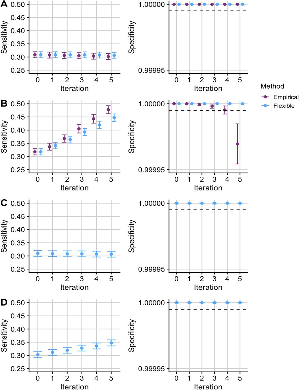
Mean +/- standard error for the sensitivity and specificity of FDR-adjusted v-values from empirical and flexible cFDR when iterating over independent (A; “simulation A”) and dependent (B; “simulation B”) auxiliary data that is bounded by [0, 1]. Panels C and D show the results from flexible cFDR when iterating over independent (C; “simulation C”) and dependent (D; “simulation D”) auxiliary data simulated from bimodal mixture normal distributions. Iteration 0 corresponds to the original FDR-adjusted p-values. Sensitivity is calculated as the proportion of SNPs with r2 ≥ 0.8 with a causal variant, that were detected with an FDR less than 5 × 10⁻⁶. Specificity is calculated as the proportion of SNPs with r2 ≤ 0.01 with all the causal variants, that were not detected with an FDR less than 5 × 10⁻⁶. A dashed line is shown where specificity = 1 − 5 × 10⁻⁶. Results were averaged across 1,000 simulations.
For simulations A and B, we could compare flexible cFDR performance to the current method, empirical cFDR24, since q ∈ [0, 1]. Performance was similar for simulation A, whilst for simulation B, the sensitivity increased across iterations more so for empirical cFDR than flexible cFDR, but this was at the expense of a greater decrease in the specificity for empirical cFDR (Figure 1B). Indeed, flexible cFDR controlled the FDR across iterations but empirical cFDR did not. This contrasts with earlier results for empirical cFDR, which showed good control of specificity24, and reflects the structure of our simulations which assume dependence between different realisations of q.
A leave-one-out procedure is required for the empirical cFDR method, as it utilises empirical CDFs and including an observation when estimating its own L-curve causes the curve to deviate around the observed point24. Flexible cFDR does not require a leave-one-out procedure as KDEs are used instead of empirical CDFs. Additionally, flexible cFDR is quicker to run than empirical cFDR, taking approximately 3 minutes compared to empirical cFDR which takes approximately 6 minutes to complete a single iteration on 80,356 SNPs (using one core of an Intel Xeon E5-2670 processor running at 2.6GHz). Together, these findings indicate that flexible cFDR performs no worse than empirical cFDR in use-cases where both methods are supported.
We anticipate that flexible cFDR will typically be used to leverage functional genomic data iteratively and it is helpful that specificity is maintained in simulations B and D. However, it is obvious that repeated conditioning on the same data would produce erroneous results, with SNPs with a modest p but extreme q incorrectly attaining greater significance with each iteration. For strictest validity, we require  as the v-value from iteration I will contain some information about qi, and the cFDR assumes
  at the next iteration. However, even when
  , we expect the dependence between v and q to be quite weak, hence the proper FDR control in simulations B and D above.
Given the wealth of functional marks available for similar tissues and cell types (for example subsets of peripheral immune cells), we wanted to assess robustness of our procedure to more extreme dependence by repeatedly iterating over auxiliary data that is capturing the same functional mark. Simulation E showed that the sensitivity increased with each iteration at the expense of a drop in the specificity in later iterations (Figure 2). The drop in specificity is exacerbated when iterating over exactly the same auxiliary data in each iteration (Figure S7), as expected. We therefore recommend that care should be taken not to repeatedly iterate over functional data that is capturing the same genomic feature, and in a real data example that follows, we average over cell types which show correlated values for functional data.

Mean +/- standard error for the sensitivity and specificity of FDR-adjusted v-values from empirical and flexible cFDR when iterating over independent (A; “simulation A”) and dependent (B; “simulation B”) auxiliary data that is bounded by [0, 1]. Panels C and D show the results from flexible cFDR when iterating over independent (C; “simulation C”) and dependent (D; “simulation D”) auxiliary data simulated from bimodal mixture normal distributions. Iteration 0 corresponds to the original FDR-adjusted p-values. Sensitivity is calculated as the proportion of SNPs with r2 ≥ 0.8 with a causal variant, that were detected with an FDR less than 5 10−6. Specificity is calculated as the proportion of SNPs with r2 ≤ 0.01 with all the causal variants, that were not detected with an FDR less than 5 × 10⁻⁶. A dashed line is shown where specificity = 1 – 5 × 10⁻⁶. Results were averaged across 1,000 simulations.
4.2. Using flexible cFDR to leverage GenoCanyon scores with asthma GWAS p-values and comparing with GenoWAP
We used flexible cFDR and GenoWAP to leverage GenoCanyon scores measuring SNP functionality with asthma GWAS p-values (Table S1). At the SNP level, flexible cFDR identified 9 newly significant SNPs (rs4705950, rs9262141, rs1264349, rs2106074, rs3130932, rs9268831, rs1871665, rs1663687 and rs12900122) which had high GenoCanyon scores (mean GenoCanyon score = 0.84). Moreover, 3 SNPs (rs10210176, rs3132619 and rs3806157) that had low GenoCanyon scores (mean GenoCanyono score = 0.01) were no longer FDR significant after applying flexible cFDR. At the locus level, flexible cFDR did not identify any newly significant index SNPs.
The results from both methods were largely comparable and we compared performance using the UK Biobank data resource. Firstly, at the SNP-level, we ranked SNPs based on their raw p-value in the discovery GWAS data set32, their v-values from flexible cFDR and their posterior scores from GenoWAP. For each of the 5152 SNPs that passed FDR significance in the UK BioBank data, we compared the rank of the raw p-values in the discovery data set with (1) the rank of the (negative) posterior score from GenoWAP and (2) the rank of the v-value from flexible cFDR. We found that 61.7% had equal or improved rank after applying GenoWAP compared to 66.3% after applying flexible cFDR (82.7% of the SNPs that had an improved or equal rank were shared between the two methods). Similarly, for the 1,963,499 that were not FDR significant in UK Biobank, 44.8% had a decreased or equal rank after applying GenoWAP, compared to 47.7% when applying flexible cFDR (and 70.6% of these SNPs were shared by both methods).
Secondly, we focused on the 144 loci that passed FDR significance in the UK Biobank data set. Within each of the 144 loci, we identified the SNP with the lowest p-value and called this the “index-SNP”. For each index SNP, we compared the rank of the raw p-values in the discovery GWAS data set32 with (1) the rank of the (negative) posterior score from GenoWAP and (2) the rank of the v-value from flexible cFDR. 66.7% had an improved or equal rank after applying GenoWAP compared to 71.1% when applying flexible cFDR. 80.5% of the loci that had an improved or equal rank were shared between the two methods.
4.3. Using flexible cFDR to leverage ChIP-seq data with asthma GWAS p-values uncovers new genetic associations
In agreement with reports that GWAS SNPs are enriched in active chromatin59, we observed that H3K27ac fold change values in asthma relevant cell types were negatively correlated with asthma GWAS p-values (Figure S8). Accordingly, FDR adjusted v-values for SNPs with high H3K27ac fold-change counts in asthma relevant cell types were lower than their corresponding original FDR values, whilst those for SNPs with low H3K27ac fold-change counts in asthma relevant cell types were higher than their corresponding original FDR values (Figure 3A; Figure 3B; Figure 3C; Table S2).
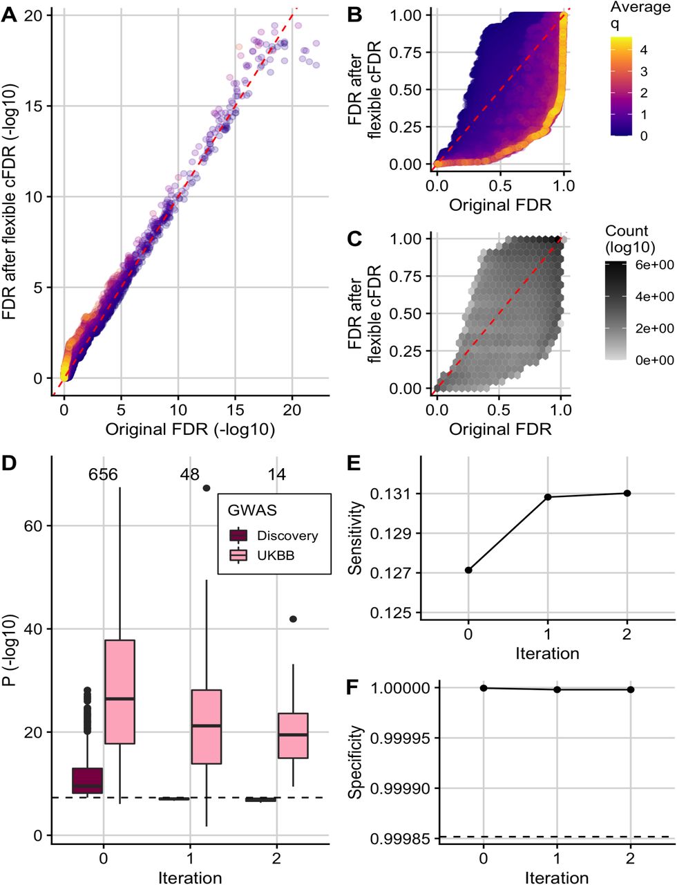
(A) (-log10) FDR adjusted v-values after 2 iterations of flexible cFDR leveraging H3K27ac counts in relevant cell types against raw (-log10) FDR adjusted p-values coloured by the average value of the auxiliary data across iterations. (B) As in A but non-log-transformed FDR values. (C) As in B but coloured by (log10) counts of data points in each hexbin. (D) Box plots of (-log10) p-values in the discovery GWAS and the UK Biobank data set for the 656 SNPs that were FDR significant in the original GWAS (Iteration 0), 48 SNPs that were newly FDR significant after iteration 1 of flexible cFDR (leveraging average H3K27ac fold change values in lymphoid and CD56 cell types) and 14 SNPs that were newly FDR significant after iteration 2 of flexible cFDR (subsequently leveraging average H3K27ac fold change values in lung tissue and CD14 cells). Black dashed line at genome-wide significance (p = 5 × 10⁻⁸). (E) Sensitivity proxy and (F) specificity proxy for the H3K27ac application results. Sensitivity proxy is calculated as the proportion of SNPs that are FDR significant in the UK Biobank data set that are also FDR significant in the original GWAS (Iteration 0), after iteration 1 of flexible cFDR or after iteration 2 of flexible cFDR. Specificity is calculated as the proportion of SNPs that are not FDR significant in the UK Biobank data set that are also not FDR significant in the original GWAS (Iteration 0), after iteration 1 of flexible cFDR or after iteration 2 of flexible cFDR. Black dashed line at 1 − 0.000148249 to show FDR control.
Overall, 656 SNPs were FDR significant in the original discovery GWAS and these have strong replication p-values in the UK Biobank data set used for validation (Figure 3D; Iteration 0). By leveraging H3K27ac data, flexible cFDR identified weaker signals that were not significant in the original data but have reassuringly small p-values in the UK Biobank data (median p-value in UK Biobank data for these SNPs is 3.54e − 20; Figure 3D). Specifically, flexible cFDR identified 48 newly significant SNPs when leveraging average H3K27ac fold change values in lymphoid and CD56 cell types (Figure 3D; Iteration 1), and an additional 14 newly significant SNPs when subsequently leveraging average H3K27ac fold change values in lung tissue and monocytes (Figure 3D; Iteration 2). The maximum p-value for these 55 newly significant SNPs in the discovery GWAS data set is 4.96e − 07 and the maximum UK Biobank p-value for these SNPs is 0.02. The newly significant SNPs had relatively small estimated effect sizes (Figure S9), implying that there may be many more regions associated with asthma with increasingly smaller effect sizes that are missed by current GWAS sample sizes.
As a proxy for sensitivity, we calculated the proportion of FDR significant SNPs in the UK Biobank data set that were also found to be FDR significant both before (“Iteration 0”) and after each iteration of flexible cFDR (Figure 3E). We found that the sensitivity increased more after iteration 1 (leveraging average H3K27ac fold change values in lymphoid and CD56 cell types) than iteration 2 (leveraging average H3K27ac fold change values in lung tissue and monocytes) and that the FDR remained controlled (Figure 3F). We also found that the order of which we iterated over the auxiliary data had minimal impact on the results (Figure S10).
At the locus level, four additional index-SNPs became significant after applying flexible cFDR (Figure 4; Table 2): rs9501077 (chr6:31167512), rs4148869 (chr6:32806576), rs9467715 (chr6:26341301) and rs167769 (chr12:57503775). Three of the four (rs4148869, rs9467715 and rs167769) validated in the UK Biobank data set at Bonferroni corrected significance (for 4 tests the Bonferroni corrected significance threshold corresponding to α = 0.05 is 0.05/4 = 0.0125).
Details of index SNPs that became newly FDR significant (FDR < 0:000148249) after using flexible cFDR to leverage H3K27ac fold change values with asthma GWAS p-values. Table contains the rsIDs (SNP), genomic positions (Chr: chromosome, BP: base pair), reference (Ref) and alternative (Alt) alleles, log ORs (beta), standard errors (SE) and p-values from the discovery GWAS, mean H3K27ac fold change values across asthma relevant cell types, p-values from UK Biobank (p UKBB) and resultant v-values from flexible cFDR. For the original p-values (and v-values), the corresponding FDR values are also given, calculated using the Benjamini-Hochberg procedure.

Manhattan plots of − log10(FDR) values before (A) and after (B) applying flexible cFDR leveraging H3K27ac counts in asthma relevant cell types. Points are coloured by chromosome and red points indicate the 4 index SNPs that are newly identified as FDR significant by flexible cFDR (rs9501077 (chr6:31167512), rs4148869 (chr6:32806576), rs9467715 (chr6:26341301) and rs167769 (chr12:57503775)). Zoomed in Manhattan plots show the genomic region containing the MHC (chr6:25477797-33448354) to show the 3 independent signals. Black dashed line at FDR significance threshold (−log10(0.000148249)).
SNPs rs9501077 and rs4148869 reside in the major histocompatibility complex (MHC) region of the genome, which is renowned for its strong long-range LD structures that make it difficult to dissect genetic architecture in this region. rs9501077 and rs4148869 are in linkage equilibrium (r2 = 0.001), and are in very weak LD with the index-SNP for the whole MHC region (rs9268969; FDR = 7.35e − 15; r2 = 0.005 and r2 = 0.001 respectively). rs9501077 (p = 1.53e − 07) has relatively high H3K27ac counts in asthma relevant cell types (mean percentile is 90th) and flexible cFDR uses this extra disease-relevant information to increase the significance of this SNP beyond the significance threshold (FDR before flexible cFDR = 3.99e − 04, FDR after flexible cFDR = 6.36e − 05; Table 2). rs9501077 is found in the long non-coding RNA (lncRNA) gene, HCG27 (HLA Complex Group 27), which has been linked to psoriasis60, however this SNP did not replicate in the UK Biobank data (UK Biobank p = 0.020).
SNP rs4148869 has very high H3K27ac fold change values in asthma relevant cell types (mean percentile is 99.6th) and so flexible cFDR decreases the FDR value for this SNP from 9.28e−04 to 7.96e − 05 when leveraging this auxiliary data (Table 2). This SNP is a 5’ UTR variant in the TAP2 gene. The protein TAP2 assembles with TAP1 to form a transporter associated with antigen processing (TAP) complex. The TAP complex transports foreign peptides to the endoplasmic reticulum where they attach to MHC class I proteins which in turn navigate to the surface of the cell for antigen presentation to initiate an immune response61. Studies have found TAP2 to be associated with various immune-related disorders, including autoimmune thyroiditis and type 1 diabetes62,63. It has also been linked to pulmonary tuberculosis in Iranian populations64. Recently, Ma and colleagues65 identified three cis-regulatory eSNPS for TAP2 as candidates for childhood-onset asthma risk (rs9267798, rs4148882 and rs241456). One of these (rs4148882) is present in the asthma GWAS data set used for our analysis (FDR = 0.12) and is in weak LD with rs4148869 (r2 = 0.4).
SNP rs9467715 is a regulatory region variant with a raw p-value that is very nearly significant in the original GWAS (p = 8.96e − 08; FDR = 2.49e − 04 compared with FDR threshold of 1.48e − 04 used to call significant SNPs). This SNP has moderate H3K27ac fold change values in asthma relevant cell types (mean percentile is 67.9th) so that when these are leveraged using flexible cFDR, the SNP is just pushed past the FDR significance threshold (FDR after flexible cFDR = 1.37e − 04; Table 2).
SNP rs167769 has a borderline FDR value in the original GWAS discovery data set (FDR = 4.04e − 04) but was found to be significant in the multi-ancestry analysis in the same manuscript (FDR = 1.61e − 05)32. This SNP has very high H3K27ac fold change values in asthma relevant cell types (mean percentile is 98.4th) and flexible cFDR decreases the FDR value for this SNP to 4.34e − 05 when leveraging this auxiliary data (Table 2). rs167769 is an intron variant in STAT6, a gene that is activated by cytokines IL-4 and IL-1366,67 to initiate a Th2 response and ultimately inhibit transcribing of innate immune response genes68,69. Transgenic mice over-expressing constitutively active STAT6 in T cells are predisposed towards Th2 responses and allergic inflammation70,71 whilst STAT6 -knockout mice are protected from allergic pulmonary manifestations72. Accordingly, rs167769 is strongly associated with STAT6 expression in the blood73–75 and lungs76 and is associated with increased risk of childhood atopic dermatitis77,78, which often progresses to allergic airways diseases such as asthma in adulthood. No genetic variants in the STAT6 gene region (chr12:57489187-57525922) were identified as significant in the original GWAS, and only rs167769 was identified as significant after leveraging H3K27ac data using flexible cFDR (Figure S11).
One significant index SNP was no longer significant after applying flexible cFDR. rs12543811 is located between genes TPD52 and ZBTB10 and has moderate H3K27ac fold change values in asthma relevant cell types (mean percentile is 52th). This SNP only just exceeds the FDR significance threshold in the original GWAS (FDR = 1.08e − 04 compared with FDR threshold of 1.48e − 04 used to call significant SNPs) but by leveraging its H3K27ac fold change values using flexible cFDR, the resultant v-value is just below the significance threshold (FDR after flexible cFDR = 3.03e − 04; Figure S12). This SNP is in strong LD with rs7009110 (r2 = 0.79) which has previous been associated with asthma plus hay fever but not with asthma alone79. Conditional analyses show that these two SNPs represent the same signal which is likely to be associated with allergic asthma32. rs12543811 was found to be significant in the UK Biobank data (UK Biobank p = 1.42e − 19).
4.4. Comparison with FINDOR, which leverages annotations from the baseline-LD model
We compared results from flexible cFDR when leveraging data for a single histone modification in several relevant cell types with results from FINDOR, which leverages a wider range of non-cell-type-specific functional annotations (Table S3). FINDOR identified 118 newly FDR significant SNPs which had a median p-value of 4.44e − 15 in the UK Biobank validation data, but the maximum UK Biobank p-value for these 55 newly significant SNPs was 0.98 (Figure 5A; Figure 5B). The proportion of FDR significant SNPs in the UK Biobank data set that were also FDR significant in the discovery GWAS data set increased from 0.127 to 0.146 and the FDR remained controlled (Figure 5C; Figure 5D).

(A) (-log10) Re-weighted p-values from FINDOR against (-log10) raw asthma GWAS p-values before re-weighting coloured by FINDOR weights. (B) Box plots of (-log10) p-values in the discovery GWAS data set and the UK Biobank data set for the 656 SNPs that were FDR significant in the original GWAS (“before”) and 118 newly significant SNPs after re-weighting using FINDOR (“after”). Black dashed line at genome-wide significance threshold (5 × 10⁻⁸). (C) Sensitivity and (D) specificity proxies for the FINDOR results. Sensitivity proxy is calculated as the proportion of SNPs that are FDR significant in the UK Biobank data set that are also FDR significant in the original GWAS or after p-value re-weighting using FINDOR. Specificity is calculated as the proportion of SNPs that are not FDR significant in the UK Biobank data set that are also not FDR significant in the original GWAS or after p-value re-weighting using FINDOR. Black dashed line at 1 − 0.000148249 to show FDR control. Manhattan plots of FDR values before (E) and after (F) re-weighting by FINDOR. Red points indicate the two index SNPs that are newly identified as FDR significant by FINDOR (rs13018263 (chr2:103092270) and rs9501077 (chr6:31167512)). Black dashed line at FDR significance threshold (−log10(0.000148249)).
At the locus level, FINDOR identified two newly FDR significant index SNPs: rs13018263 (chr2:103092270; original FDR = 6.79e − 04, new FDR = 1.00e − 04) and rs9501077 (chr6:31167512; original FDR = 3.99e − 04, new FDR = 4.86e − 05) (Figure 5E; Figure 5F). SNP rs13018263 is an intronic variant in SLC9A4 and is strongly significant in the UK Biobank validation data set (p = 4.78e − 31). Ferreira and colleagues80 highlighted rs13018263 as a potential eQTL for IL18RAP, a gene which is involved in IL-18 signalling which in turn mediates Th1 responses81, and is situated just upstream of SLC9A4. Genetic variants in IL18RAP are associated with many immune-mediated diseases, including atopic dermatitis82 and type 1 diabetes83. Interestingly, although different auxiliary data was leveraged using flexible cFDR and FINDOR in our analyses, both methods found index SNP rs9501077 to be newly significant, but this is not validated in the UK Biobank data (UK Biobank p = 0.020).
Two additional index SNPs were found to be no longer significant after re-weighting by FINDOR, rs2589561 (chr10:9046645; original FDR = 5.25e − 05, new FDR = 3.06e − 03) and rs17637472 (chr17:47461433; original FDR = 1.42e − 05, new FDR = 9.42e − 04), however both of these SNPs were strongly significant in the UK Biobank validation data set (p = 2.09e − 29 and p = 1.75e − 14 respectively).
SNP rs2589561 is a gene desert that is 929kb from GATA3, a transcription factor of the Th2 pathway which mediates the immune response to allergens32,84. Hi-C data in hematopoietic cells showed that two proxies of rs2589561 (r2 > 0.9) are located in a region that interacts with the GATA3 promoter in CD4+ T cells85, suggesting that rs2589561 could function as a distal regulator of GATA3 in this asthma relevant cell type. rs2589561 has relatively high H3K27ac fold change values in the asthma relevant cell types leveraged by flexible cFDR (mean percentile is 85th) and flexible cFDR decreased the FDR value from 5.25e − 05 to 2.78e − 05.
SNP rs17637472 is a strong cis-eQTL for GNGT2 in blood73–75,86, a gene whose protein product is involved in NF-κB activation87. This SNP has moderate H3K27ac fold change values in relevant cell types (mean percentile is 62th) and the FDR values for this SNP were similar both before and after using flexible cFDR to leverage the H3K27ac data (original FDR = 1.42e − 05, new FDR = 1.35e − 05).
5. Discussion
Developments in experimental protocols have enabled researchers to decipher the functional effects of various genomic signatures. We are now in a position to prioritise sequence variants associated with various phenotypes not just by their genetic association statistics but also based on our biological understanding of their functional role. Originally developed to leverage test statistics from genetically related traits, we have extended the existing cFDR framework to support auxiliary data from arbitrary continuous distributions. Our extension, flexible cFDR, provides a statistically robust framework to leverage functional genomic data with genetic association statistics to boost power for GWAS discovery.
Whilst larger case and control cohort sizes will also boost statistical power for GWAS discovery, incorporating functional data provides an additional layer of biological evidence that an increase in statistical power alone cannot provide. Moreover, there are instances in the rare disease domain where case sample sizes are restricted by the recruitment of cases. Our method has potential utility in instances where limited sample sizes are restrictive, as it provides an alternative approach to increase statistical power.
Our approach differs from competing GWAS signal prioritisation methods as it outputs quantities analogous to p-values that are readily interpretable, enable control of type-1 error rate and permit multiple iterations leveraging multiple auxiliary data sets. Based on a method with firm theoretical grounding for FDR control24, our method intrinsically evaluates the relevance of the auxiliary data by comparing the joint probability density of the test statistics and the auxiliary data to the joint density assuming independence, and can therefore be used to inform researchers of relevant functional signatures and cell types. Choice of functional data to use may be guided by prior knowledge, or in a data driven manner using a method such as GARFIELD88 to quantify the enrichment of GWAS signals in different functional marks.
Our method has several limitations. Firstly, care must be taken to ensure that the auxiliary data to be leveraged iteratively is capturing distinct disease-relevant features to prevent multiple adjustment using the same auxiliary data. The definition of “distinct disease-relevant features” to leverage is at the user’s discretion and sparks an interesting philosophical discussion. For example, leveraging data iteratively from various genomic assays measuring the same genomic feature at different resolutions may be deemed invalid for some researchers but valid for others, since if the mark is repeatedly identified by different assays then it is more likely to be reliably present. Whilst we show that our method is robust to minor departures from  , this does not extend to strongly related q. We would argue that the conservative approach would be to average over correlated auxiliary data, to ensure that the q vectors are not strongly correlated.
Secondly, the cFDR framework assumes a monotonic relationship between the test statistics and the auxiliary data: specifically, low p-values are enriched for low values in the auxiliary data. Our method automatically calculates the correlation between p and q and if this is negative then the auxiliary data is transformed to q := −q. However, if the relationship is non-monotonic (for example low p-values are enriched for both very low and very high values in the auxiliary data) then the cFDR framework cannot simultaneously shrink v-values for these two extremes. This non-monotonic relationship is unlikely when leveraging single functional genomic marks, but may occur if, for example, multiple marks were decomposed via PCA. We therefore recommend that users use the ‘corr_plot’ function in the ‘fcfdr’ R package to visualise the relationship between the relationship between the two data types. Note that this restriction could be removed if we used density instead of distribution functions, and worked at the level of ‘local FDR’37, but this would in turn reduce the robustness our method has to data sparsity in the (p, q) plane.
Finally, in our asthma application we only leveraged data for a single histone modification across various cell types. Additional data measuring other histone modifications (e.g. repressive marks) could also be leveraged to further increase power.
We compared our method to other GWAS prioritisation methods that leverage functional data, GenoWAP and FINDOR. GenoWAP is GWAS signal prioritsation method that integrates genomic functional annotation and GWAS test statistics to generate posterior scores of disease-specific functionality17. For each SNP, the mean GenoCanyon score (or tissue-specific GenoSkyline89/ GenoSkyline-Plus90 score) of the surrounding 10,000 base pairs is used as the prior probability in the model, restricting its utility to leveraging these scores as the auxiliary data. The results were similar for flexible cFDR and GenoWAP when leveraging GenoCanyon scores, but rather unexciting, as no newly FDR significant index SNPs were identified. We suggest that this is due to the one-dimensional non-trait-specific auxiliary data that is being leveraged, which is unlikely to capture enough disease relevant information to substantially alter conclusions from a study.
FINDOR is a p-value reweighting method that bins data to derive bin-specific weights. FINDOR bins data according to the values of the expected χ2 statistics and recommends course binning (so that in the asthma analysis, the average number of SNPs in each bin was 19763). The method uses the BaselineLD model55 for prediction, requiring users to (i) download pre-computed LDscores and (ii) run LD-score regression on their GWAS data to obtain annotation effect size estimates prior to running FINDOR. Although 96 annotations were leveraged with asthma p-values using FINDOR, compared to 2 annotations (comprised of averaged H2K27ac counts in 13 cell types) leveraged using flexible cFDR, flexible cFDR identified more associations that could be validated in the UK Biobank data. The difference emphasises the importance of being able to iterate over different auxiliary measures, and suggests that a fruitful area of extension for cFDR will be to increase the robustness of FDR control for dependent q.
Overall, we anticipate that flexible cFDR will be a valuable tool to leverage functional genomic data with GWAS test statistic to boost power for GWAS discovery.
7. Description of Supplemental Data
Supplemental data includes 12 figures and 3 tables.
8. Declaration of Interests
Anna Hutchinson is a GSK-sponsored iCASE student.
10. Web Resources
Code to reproduce results from this manuscript https://github.com/annahutch/fcfdr_manuscript
Flexible cFDR software https://github.com/annahutch/fcfdr
Empirical cFDR software https://github.com/jamesliley/cfdr/
GWAS Catalog https://www.ebi.ac.uk/gwas/
Asthma GWAS summary statistics ftp://ftp.ebi.ac.uk/pub/databases/gwas/summary_statistics/DemenaisF_29273806_GCST006862/harmonised/29273806-GCST006862-EFO_0000270.h.tsv.gz
Neale lab UK Biobank http://www.nealelab.is/uk-biobank
Neale lab asthma summary statistics https://www.dropbox.com/s/kp9bollwekaco0s/20002_1111.gwas.imputed_v3.both_sexes.tsv.bgz?dl=0
NIH Roadmap data resource https://www.ncbi.nlm.nih.gov/geo/roadmap/epigenomics/?search=pbmc&display=200
NIH Roadmap H3K27ac data resource https://egg2.wustl.edu/roadmap/data/byFileType/signal/consolidated/macs2signal/foldChange/
FINDOR software https://github.com/gkichaev
GenoCanyon annotations http://genocanyon.med.yale.edu/GenoCanyon_Downloads.html GenoWAP software https://github.com/rlpowles/GenoWAP-V1.2
11. Data and Code Availability
The code generated during this study are available at https://github.com/annahutch/fcfdr. The source data for figures/analysis in the paper is available https://github.com/annahutch/fcfdr_manuscript.
9. Acknowledgments
This research was funded by Engineering and Physical Sciences Research Council (EP/R511870/1 to A.H.), GlaxoSmithKline (GSK; to A.H.), Wellcome Trust (WT107881 to C.W. and G.R.) and Medical Research Council (MC UU 00002/4 to C.W.).
References
- 1.↵
- 2.↵
- 3.↵
- 4.↵
- 5.↵
- 6.↵
- 7.↵
- 8.↵
- 9.
- 10.
- 11.
- 12.
- 13.↵
- 14.
- 15.↵
- 16.
- 17.↵
- 18.
- 19.
- 20.
- 21.↵
- 22.↵
- 23.↵
- 24.↵
- 25.↵
- 26.
- 27.↵
- 28.↵
- 29.↵
- 30.↵
- 31.↵
- 32.↵
- 33.↵
- 34.↵
- 35.↵
- 36.↵
- 37.↵
- 38.↵
- 39.↵
- 40.↵
- 41.↵
- 42.↵
- 43.↵
- 44.↵
- 45.↵
- 46.↵
- 47.
- 48.
- 49.
- 50.↵
- 51.↵
- 52.↵
- 53.↵
- 54.↵
- 55.↵
- 56.↵
- 57.↵
- 58.↵
- 59.↵
- 60.↵
- 61.↵
- 62.↵
- 63.↵
- 64.↵
- 65.↵
- 66.↵
- 67.↵
- 68.↵
- 69.↵
- 70.↵
- 71.↵
- 72.↵
- 73.↵
- 74.
- 75.↵
- 76.↵
- 77.↵
- 78.↵
- 79.↵
- 80.↵
- 81.↵
- 82.↵
- 83.↵
- 84.↵
- 85.↵
- 86.↵
- 87.↵
- 88.↵
- 89.↵
- 90.↵


