

Abstract
Predictive coding represents a promising framework for understanding brain function. It postulates that the brain continuously inhibits predictable sensory input, ensuring a preferential processing of surprising elements. A central aspect of this view is its hierarchical connectivity, involving recurrent message passing between excitatory bottom-up signals and inhibitory top-down feedback. Here we use computational modelling to demonstrate that such architectural hard-wiring is not necessary. Rather, predictive coding is shown to emerge as a consequence of energy efficiency. When training recurrent neural networks to minimise their energy consumption while operating in predictive environments, the networks self-organise into prediction and error units with appropriate inhibitory and excitatory interconnections, and learn to inhibit predictable sensory input. Moving beyond the view of purely top-down driven predictions, we demonstrate via virtual lesioning experiments that networks perform predictions on two timescales: fast lateral predictions among sensory units, and slower prediction cycles that integrate evidence over time.
1 Introduction
In computational neuroscience and beyond, predictive coding has emerged as a prominent theory for how the brain encodes and processes sensory information (Srinivasan et al., 1982; Mumford, 1992; Friston, 2005; Clark, 2013). It postulates that higher-level brain areas continuously keep track of the causes of lower-level sensory input, and actively inhibit incoming sensory signals that match expectation. Over time, the brain’s higher-level representations are shaped to yield increasingly accurate predictions that in turn minimise the surprise that the system encounters in its inputs. That is, the brain creates an increasingly accurate model of the external world and focuses on processing unexpected sensory events that yield the highest information gain.
Adding to the increasing, albeit often indirect, experimental evidence for predictive coding in the brain (Alink et al., 2010; Näätänen et al., 2001; Summerfield et al., 2011, 2008; Squires et al., 1975; Hupé et al., 1998; Murray et al., 2002; Rao et al., 2016; Kok et al., 2012; Ekman et al., 2017; De Lange et al., 2018; Dijkstra et al., 2020; Schwiedrzik and Freiwald, 2017), computational modelling has investigated explicit implementations of predictive coding, indicating that they can reproduce experimentally observed neural phenomena (Rao and Ballard, 1999; Lee and Mumford, 2003; Friston, 2005, 2010). For example, Rao and Ballard (1999) demonstrated that a hierarchical network with top-down inhibitory feedback can explain extra-classical field effects in V1. In addition, deep neural network architectures wired to implement predictive coding were shown to work at scale in real-world tasks (Chalasani and Principe, 2013; Lotter et al., 2016; Villegas et al., 2017; Lotter et al., 2020), adding further support for the computational benefits of recurrent message passing (Spoerer et al., 2020; Kietzmann et al., 2019; Kar et al., 2019; Linsley et al., 2020; Spoerer et al., 2017; van Bergen and Kriegeskorte, 2020). The common rationale of modelling work focused on predictive coding is to test for its computational and representational effects by hard-wiring the model circuitry to mirror hierarchical and inhibitory connectivity between units that drive predictions, and units that signal deviations from said predictions (also termed sensory, or error units).
Contrasting this approach, we here ask a different question: can computational mechanisms of predictive coding naturally emerge from other, perhaps simpler, computational principles? In search for such principles, we take inspiration from the organism’s limited energy budget. Expanding on previous work on efficient coding and sparse coding (Barlow et al., 1961; Bell and Sejnowski, 1995; Olshausen and Field, 1996; Bialek et al., 2006; Berkes and Wiskott, 2005; Chalk et al., 2018; Eckmann et al., 2020), we subject recurrent neural networks (RNNs) to predictable sequences of visual input and optimise their synaptic weights to minimise what constitutes the largest source of energy consumption in biological systems: action potential generation and synaptic transmission (Sengupta et al., 2010). We then test the resulting networks for phenomena typically associated with predictive coding. We compare the energy budget of the networks to theoretically-determined lower bounds, search for inhibitory connectivity profiles that mirror sensory predictions, and explore whether the networks automatically separate their neural resources into prediction and error units.
2 Results
To better understand whether, and under which conditions, predictive coding may emerge in energy-constrained neural networks, we trained a set of RNNs on predictable streams of visual input. For this, we created sequences of MNIST digits (LeCun et al., 1998) iterating through 10 digits in numerical (category) order. Starting from a random digit, sequences wrapped around from nine to zero. The visual input to each network unit was stimulus-dependent, with each unit receiving an input which mirrored its corresponding pixel intensity. These visual inputs were not weighted and thus we prevented the models from learning to ignore the input as a shortcut to a solution for energy efficiency. Instead, we hypothesised that the models would learn to use their recurrent connectivity to counteract the input drive where possible, and thereby to minimise their energy consumption. Energy costs were defined to arise from synaptic transmission and action potentials, thereby mirroring the two most dominant sources of energy consumption in neural communication (Sengupta et al., 2010). Figure 1 shows an overview of the experimental pipeline.

Overview of the model architecture and input pipeline. The upper part of the figure shows an example input sequence fed to a recurrent network. 10 MNIST digits are presented in ascending order to the network (with wraparound after digit 9). The lower part of the figure shows that each pixel drives one unit. The preactivation of a single unit constitutes the sum of the recurrent activity into the unit and the input drive determined by the intensity of the pixel that it is connected to. The output of the network is determined by taking the ReLU of the preactivations of the network units.
2.1 Preactivation as a proxy for the energy demands of the brain
Sparse coding is often implemented as an L1 objective on the unit outputs, i.e. networks are optimised to reduce the overall unit activity post non-linearity. However, given that synaptic transmission contributes considerable energy cost alongside action potentials, a different learning objective is required; i.e. a minimisation of unit outputs alone could be implemented via unreasonably strong inhibitory connections, which themselves might increase the overall energy budget. To solve this issue, we propose to instead train energy-efficient RNNs by minimising absolute (L1) unit preactivation. This has two desired properties. First, it drives unit output towards zero, mirroring a minimisation of unit firing rates (dependent naturally upon the form of activation function used). Second, we show that this objective also leads to minimal synaptic weight magnitudes in cases of noise in the system, thereby mirroring an overall reduction in synaptic transmission (see Appendix B for a theoretical derivation of why this is the case).
Following above considerations, which we regard as the first result of this paper, we confirmed that training RNNs in this manner indeed lead to a minimisation of the overall unit preactivation (i.e. a proxy for energy consumption in biological networks). We trained a total of ten network instances to ensure the generality of our results (Mehrer et al., 2020). The resulting network activity was compared to three theoretical scenarios. First, we computed the overall input drive, i.e. a scenario in which the lateral weights are removed and the RNNs are therefore completely driven by external input. This estimate measures the ‘energy’ that flows into the network from sensory sources alone. Second, we estimated the theoretical network activity if RNNs learned to predict the pixel-wise median value of the whole training data. This value represents a scenario in which the networks counteract the input drive based on the global dataset statistic, without sequence-specific categorical inhibitions. Third, we computed the theoretical activity in a best case scenario in which the RNNs learn to predict and inhibit the pixel-wise median value of the particular digit category being presented. This theoretical model has perfect knowledge of the current position in the input sequence and can therefore inhibit the matching dataset’s pixel-wise median. Given the training setup, this measure represents a lower bound on network preactivation (energy). A derivation for these bounds on performance is given in Section 4.3.
As can be seen in Figure 2, which depicts the theoretical bounds together with the average preactivation across ten trained RNN instances, the trained networks approach the optimal case with increasing network time (i.e. increasing exposure to the sequence). Whereas the RNNs cannot predict well at the first time step (they have no information about where the sequence begins), the average unit preactivation drops below the pixel-wise median of the training data after only one timestep and subsequently converge towards the category median, i.e. the lower bound. This indicates that the RNNs are able to integrate evidence over time, improving their inhibitory predictions with increasing sensory evidence for the current input state.

Evolution of the ‘energy consumption’ (mean absolute preactivation) of the trained RNNs, together with three theoretical scenarios. input: stimulation entering the networks via sensory input, median: network preactivation if the networks predicted and inhibited the (pixel-wise) median of the training data, category median: network preactivation if the networks had perfect knowledge of the current state of the sequence, and thereby inhibit the (pixel-wise) median value of the upcoming digit category. RNN: actual network preactivation. Mean preactivations shown with 95% confidence intervals, bootstrapped across 10 network instances with replacement.
2.2 RNNs trained for energy efficiency learn to predict and inhibit upcoming sensory signals
Having established that the trained RNNs successfully reduce their preactivation over time, we further confirmed a targeted inhibition of predicted sensory input, a hallmark of predictive coding, by visualising the network drive induced by the recurrent connections for a sample sequence in Figure 3 (top row: input drive, bottom row: (recurrent) internal drive, see Section 4.2 for these measures). Two observations are of importance in this example. First, the network clearly predicts and inhibits the upcoming digit category. Second, as time progresses the network is able to integrate information, leading to better knowledge of the current sequence position, and more targeted inhibitions (e.g. the inhibition of later digits appears more clear/targeted than earlier predictions). Better predictions, in turn, result in progressively lower network activity. Please note that this pattern of results is in line with hierarchical predictive coding architectures in which feedback from higher order areas is subtracted from sensory evidence of lower areas. However, no such hierarchical organisation was imposed in our RNNs. Rather, all effects emerge due to optimisation of the networks for energy efficiency.

Network activity for an example sequence. The RNN units are organised according to the locations of their input pixels. Row 1 shows the input drive xt and row 2 shows the recurrent drive pt. Excitatory signals are depicted in red, while inhibitory signals are depicted in blue. The darker the colour the stronger the signal. The sequence images shown were not used for training. The observable improvements in inhibitory network drive indicate that the RNN integrates sensory evidence over time, leading to better internal knowledge of the state of the world
2.3 Separate error units and prediction units as an emergent property of RNN self-organisation
Our previous results demonstrate that RNNs, when optimised to reduce action potentials and synaptic transmission, exhibit key phenomena associated with predictive coding. Thus, predictive coding emerges, without architectural hard-wiring, as a result of energy efficiency in predictable sensory environments. A second key component postulated by the predictive coding framework is the existence of distinct neural populations that either provide sensory predictions, or which carry the deviations from such predictions, i.e. prediction error units (Bastos et al., 2012). Given the non-hierarchical, non-constrained nature of the current setup, we next asked whether a similar separation could also be observed in our energy efficient networks.
If the models had indeed developed separate populations of error and prediction units, they would be expected to have different activity profiles. Error units calculate the difference between the predicted input and the actual input by integrating excitatory signals from the input and inhibitory signals from prediction units. In the RNNs, this means that such units would receive excitatory signals from the input drive, and inhibitory signals from the recurrent connections. Prediction units, on the other hand, represent the internal representation of the external environment, and are updated over time as guided by the prediction errors. The prediction units are therefore expected to receive their primary input from the error units. To test for such activity patterns, we record, for an example network, the average excitatory signals from both the input and recurrent connections for each unit at the last timestep of the presented sequences. As can be seen from Figure 4, separate populations of network units can be observed in the trained network. While one population is predominantly driven by network-internal recurrent connections, another population receives its excitatory input predominantly from the sensory input.

Trained RNNs exhibit distinct populations of input driven and feedback driven units. A: comparison of mean excitatory drive from input ⟨x+⟩ and recurrent feedback ⟨p+⟩ for an example network indicates a clear separation between input-driven and feedback-driven units. B: mean excitatory drive from recurrent connections for each unit in the RNN. C: mean excitatory input drive for each unit in the RNN.
Interestingly, the two populations occupy different topographic parts in the RNN, with units driven by network internal states (i.e. prediction units) residing in locations that are typically not strongly driven by sensory input. Such secondary use of neural resources that would otherwise remain unused seems in line with neuroscientific evidence for cortical plasticity (Kaas, 2002; Merabet and Pascual-Leone, 2010).
2.4 Two distinct inhibitory mechanisms working at different timescales
As can be seen in Figures 2 and 3, the inhibitory predictions of the second timestep are less precise than later timesteps, but nevertheless contain some category specific predictions. This network behaviour is of interest, as prediction loops from input to prediction units and back require two timesteps to come into effect (one to activate prediction units and one for these prediction units to provide feedback). This suggests that the observed predictions in timestep 2 are rather driven by more immediate lateral connections among error units - to our knowledge a mode of predictive coding not previously considered. That is, we observe two different modes of predictive inhibitions. One operating at a faster timescale among error units, and one on a slower timescale involving prediction units with the potential to integrate evidence over time. This hypothesis of evidence integration via prediction units was confirmed by virtual lesion studies. As shown in Figure 5A, an un-lesioned RNN is capable of more fine-grained predictions with increasing sequence lengths leading up to the sensory input. On the other hand, a network in which (postulated) prediction units are lesioned remains fixed at the initial and immediate prediction, derived from lateral connections among error units, and is missing the ability to integrate evidence over time (see Supplemental Figures SA1 and SA2 for further lesion experiments targeting other digit categories). Prediction and error units were identified based upon the ratio of their input vs external drive (see Section 4.4).

Evidence for two mechanisms of inhibitory predictions. A: internal drive (pt) in the RNN for the ‘0’ digit category at different points in time. Each square shows the internal drive of the network at a certain point in a sequence, e.g. at ‘prec. fr.=2’ we have the internal drive after the sequence ‘8-9’ and at ‘prec. fr.=5’ we have the internal drive after the sequence ‘5-6-7-8-9’. The first row shows the predictions of a normal RNN, while the second row shows the result of lesioning RNN prediction units. Panel B: mean preactivations of normal RNN and lesioned RNNs. In contrast to normal RNNs, the lesioned RNNs do not reduce their preactivation over time, indicating that they are not capable of integrating evidence over time. Mean preactivations shown with 95% confidence intervals, bootstrapped across 10 network instances with replacement.
3 Discussion
Here, we demonstrate that recurrent neural network models, trained to minimise biologically realistic energy consumption (action potentials and synaptic transmissions), spontaneously develop hallmarks of predictive coding without the need to hardwire predictive coding principles into the network architecture. This opens up the possibility that predictive coding can be understood as a natural consequence of recurrent networks operating under a limited energy budget in predictive environments. In addition to category-specific inhibition and increasingly sharpened predictions with time, we observed that the RNNs self-organise into two distinct populations in line with error units and prediction units.
Beyond these processes, we observe two distinct mechanisms of prediction, a faster inhibitory loop among error units, and a slower predictive loop that enables RNNs to integrate information over longer timescales and thereby to generate increasingly fine-grained predictions. This observation can be interpreted as a rudimentary form of hierarchical self-organisation in which the predictive units can be viewed as a higher-order cortical population operating on longer timescales and the error units as a lower-order cortical population operating on shorter time scales. This interpretation is consistent with hierarchical predictive coding architectures such as Rao and Ballard (1999) or Lotter et al. (2016) as well as the organisation of the brain in terms of a hierarchy of timescales (Kiebel et al., 2008; Baldassano et al., 2017).
It needs to be noted that the current experiments rely on MNIST digit sequences and therefore represent a proof of concept. Future work will explore larger-scale recurrent systems and their interplay with more natural image statistics. In terms of model details, future work could also explore energy efficiency in spiking network models where membrane voltages and spike-times must be considered. In addition, how a predictive system should optimally process differing spatial and temporal scales of dynamics and deals with unpredictable but information-less inputs (e.g. chaotic inputs and random noise) are key areas for future consideration.
In summary, our current set of findings suggests that predictive coding principles do not necessarily have to be hard-wired into the biological substrate but can be viewed as an emergent property of a simple recurrent system that minimises its energy consumption in a predictable environment. Notably, we have shown here that minimising unit preactivations, under mild assumptions of noise in the system, implies minimising both unit activity and synaptic transmission. This observation opens further interesting avenues of research into efficient coding and neural network modelling.
4 Materials and methods
4.1 Data generation
The input data are sequences of images drawn from the MNIST database of handwritten digits LeCun et al. (1998). Images are of size 28 × 28 with pixel intensities in the range [0, 1]. There are 60,000 images in the training set and 10,000 images in the test set. Each set of images can be divided into 10 categories; one for each digit. The frequency of each digit category in the dataset varies slightly (frequencies lie within 9% - 11% of the total dataset (70,000 samples)). Sequences are generated by choosing random digits as starting points. Digits from numerically subsequent categories are then randomly sampled and appended to the sequence until the desired sequence length is reached. The categories are wrapped-around such that after category ‘nine’ the sequence continues from category ‘zero’. The sequence length can be chosen in advance, but all sequences are constrained to have the same length (in our simulations we take a sequence length of 10). The sequences are organised into batches. The images are drawn without replacement and the process is stopped when there are no image samples available for the next digit. Incomplete batches, in which there are no remaining image samples to complete a sequence, are discarded.
4.2 RNN architecture and training procedure
We created a recurrent neural network (RNN) consisting of N = 784 units (equivalent to the number of pixels in the input images) that are fully recurrently connected to each other. Each unit is driven by an input signal. The equations that determine the RNN dynamics are:


 where xt ∈ ℝN denotes the input drive, at ∈ ℝNdenotes the preactivation, W ∈ ℝN ×N denotes the recurrent weight matrix of the RNN (the only learnable parameters),pt ∈ ℝN denotes the recurrent feedback, and ht ∈ ℝN the unit outputs (in our study f is the ReLU non-linearity). The subscripts, t and t − 1, refer to the discrete (integer) timestep of the system since all of these variables (aside from the weights) are iteratively updated. The weight matrix is uniformly initialised in [−1, 1] and scaled by
  , i.e. proportionally scaled by the number of units in the weight matrix.
The objective of minimising energy is captured through the following loss function:
 where T is the number of time steps, N is the number of units, and at is the preactivation of the units when processing the t-th element (or timestep) in a given sequence. We trained 10 model instances for 200 epochs with batch-size 32 (32 sequences per batch) with the Adam optimiser (β 1 = 0.9, β2 = 0.999, learning rate = 0.0001) (Kingma and Ba, 2014). Model training differed in weight initialisation and training sequence. We tested these same 10 model instances (lesioned models in figure 5 panel B) but with unit activity ht−1 masked such that the feedback driven units did not affect the computation of at. No extensive hyperparameter search was performed. The models were trained using PyTorch 1.4.0 and Python 3.7.6.
4.3 Derivation and calculation of bounds on preactivation
To benchmark how well the model minimises preactivation we derived three reference measures. These were: the input activity alone (i.e. no prediction), the pixel-wise median of the entire dataset removed from each image, and the pixel-wise median by digit category removed from each image. To relate these benchmarks to prediction, consider that the loss function, Equation 4, measures the L1-norm of the preactivation. This preactivation is composed of the input drive and some recurrent input. Now consider that this recurrent input can be an inhibition (i.e. negatively signed) which cancels the input drive and minimises this loss. Given this consideration, we can state the three benchmarks for performance, e1, e2, e3, as (inhibitory feedback) prediction of three forms:


 where X ∈ ℝN × M is the entire (MNIST) dataset (of digits), X(c)∈ ℝN×M(c) denotes the M(c) data points that belong to (image) category c and
  denotes the pixel-wise median of a dataset X. In this formulation, e1 reflects the loss computed based upon input activity induced by xt without any attempt of suppression by the RNN, e2 is the loss based upon residue activity left after subtracting the (pixel-wise) median intensity of the entire dataset, and e3 is the loss based upon residue activity left after subtracting the (pixel-wise) median intensity of that image category c. To understand why these specific (pixel-wise median) benchmarks make sense we have to understand what the optimal behaviour is under the loss function.
Our loss function, Equation 4, is an L1 norm on the preactivation of the units of our network. This preactivation consists of a (fixed) input drive which is modified by recurrent inputs. We can therefore consider, what form of recurrent contribution would minimise this L1 norm. Lets suppose that our model (and therefore recurrent contribution) has perfect knowledge of the category of the upcoming input, labelled below c. Disregarding the temporal element of our RNN, and considering minimisation of a single timestep input, let us label b ∈ ℝN as our estimation of the recurrent (inhibitory) contribution. The loss, summed across all samples of the category c, is given by:
 where m now indexes the set of examples of stimuli in category c (stimuli labelled
  ) of which there are a total of M(c) samples. Note that this summing is required since despite knowledge of the category c’s upcoming presentation, the specific sample from within this category is unknown and all samples are equally likely. Thus, to minimise the loss across all possible outcomes we minimise their summation.
The value for the recurrent contribution (b) that minimises this equation is given by:

This equation is satisfied when the number of cases in which the data is greater than the recurrent contribution  is precisely equivalent to the number of cases in which the data is smaller than the recurrent contribution
  . This must be true at a pixel-wise level (i.e. for each element of the vectors
  and b). These inequalities are consistent when our estimation is equal to the the median pixel value (per pixel) of the respective category in the dataset
  . Hence, this is the prediction which would minimise our L1 loss function given the constraint of random sampling of images from each category (our benchmark e3 above). The above derivation supposed that the model had perfect knowledge of the category of upcoming samples. However, if the model was not capable of identifying which category it should expect, the best it could do would be to predict the median of the entire dataset. This forms another of our benchmarks on performance (e2).
The model preactivations in Figures 2 and 5 panel B are averaged over 891 sequence presentations from the test data. The benchmarks that we have produced here, e1, e2, e3, are computed over the entire training dataset (60,000 MNIST Images), or per category (as in e2), and the outcome of these estimations are applied to the individual digits in each of the (891) sequences and averaged by time-step. Each data point of model preactivation represents the mean over 10 model instances. Error bars are determined with 95% confidence intervals, bootstrapped with replacement over 10000 repetitions. Each data point of the theoretical bounds is likewise determined over 10 model instances with 95% confidence intervals, bootstrapped with replacement over 10000 repetitions. The variance in the bounds is due to the variation in input sequence generation and presentation across the 10 models. The variation for model preactivation is in addition to that driven by variation in weight initialisation.
4.4 Determination of predictive and error units
In order to determine whether units were primarily driven by feedback or input in Figure 4 we divided the test set into K = 891 sequences of length T = 10 and processed them through the trained RNNs. For a particular unit n, we calculated the input drive  and recurrent feedback drive
  by taking the rectifier of the input and feedback at the final time point and averaging them over the sequences

 where
where  is the value of the pixel that drives the unit in the k-th sequence at time point T and
  is the activity induced by reciprocal connectivity in the k-th sequence at time point T. We classified a unit as input driven if
  and feedback driven if
  .
.
6 Data availability
All data and analysis code along with instructions is available at: https://github.com/KietzmannLab/EmergentPredictiveCoding
Appendix A: supplementary figures
Supplementary figures accompanying Predictive coding emerges in energy efficient recurrent neural networks.

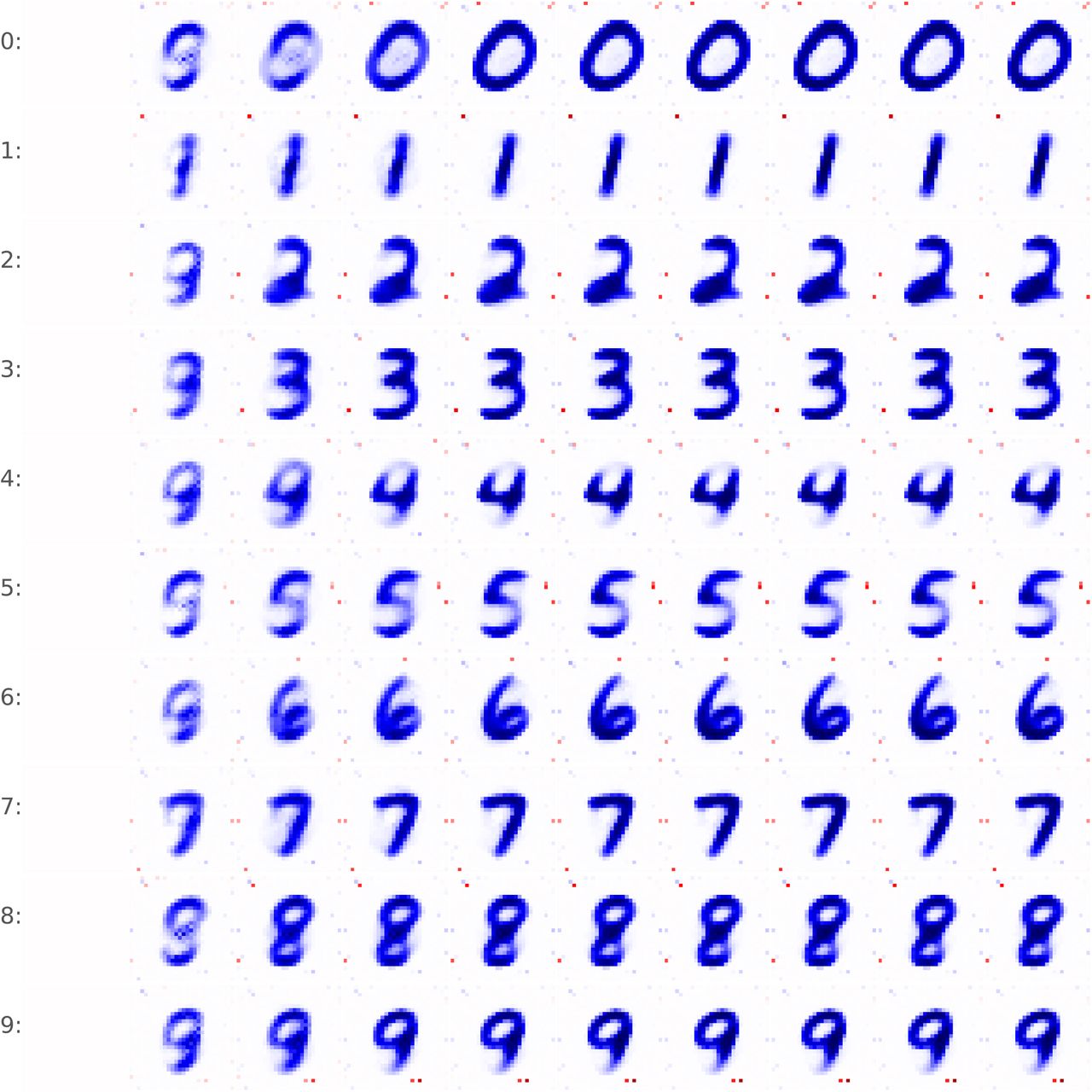
Recurrent feedback (pt) in the RNN for different input categories at different points in time. Each row shows the recurrent feedback at the step with a specific input category will be expected. Each column shows the recurrent feedback after a different number of preceding images in the sequence. The inhibitory effect (i.e. predictions) gets more pronounced as sequences progress.

Recurrent feedback (pt) in the lesioned RNN model for different input categories at different points in time. Each row shows the recurrent feedback at the step with a specific input category will be expected. Each column shows the recurrent feedback after a different amount of preceding images in the sequence. The inhibitory effect with lesioned prediction units is weak and remains constant throughout the sequence.
Appendix B: theoretical motivation for preactivation
Supplementary material accompanying Predictive coding emerges in energy efficient recurrent neural networks.
This supplement provides a derivation for the claim in the main manuscript that minimising preactivation leads to smaller weights and thus synaptic transmission. We do this by analysing what weight changes are induced in the case where noise causes predictions to deviate from the optimal predictions.
Parameter updates induced by our L1 loss function
Here we consider the form of weight updates for the system described in this paper (see Materials and methods for extended description).
In short, consider a dataset M of samples, each of dimension N, X ∈ ℝM×N, where the individual samples, indexed m, are labelled xm ∈ ℝN The individual units of our system are each driven by a single element of some sampled input data and also receive some feedback from recurrent projections. Thus, we can formulate the preactivation of a given unit, indexed i in our system as xmi−bi, where bi is the recurrent feedback computed as bi = ∑j wji hj. The loss function of our system aims to minimise the L1 norm of this preactivation. We are interested in the form of the weight updates over all possible input drives which might appear (note the specific input stimulus is randomly chosen from within a category for our main paper).
Given this setup, we can frame an L1 loss function (which is used to train our system) for this particular unit as:

This L1 loss is computed over all possible input samples following some network dynamic up to that moment. The minimum of this equation is reached when the derivative of this equation is 0. That is,

If we rewrite |xmi − bi| as  We can write out the derivative as:
 where u =(xmi−bi)2, and v = xmi − bi We obtain
 and the derivative,
  , would be at zero (and therefore the loss function at a minimum) when we have an equal number of cases in which the feedback projection is greater than versus less than the data (i.e. the sum over signs would be zero). This would be achieved by setting the recurrent feedback equal to the median value of the entire input datasets, bi = µ1/2(Xi), where Xi is the set of all th elements of our samples, Xi∈ℝM×1.
In addition to this analysis we can also compute the derivative with respect to a specific recurrent projecting weights from a pre-synaptic unit indexed j) as:

Note our ability to extract the recurrent activation, hj, from the summation since we assume the network past is fixed and we are computing its loss over all possible ‘next’ samples.
The effect of noise in the recurrence
Ideally bi = µ1/2(Xi),, but due to noise in the recurrent prediction, bi can diverge from this optimum. We will describe below how the loss will be minimised in this instance by first rewriting the recurrence into its positive and negative terms. Remember that we formulate our parameter bi as being determined by the transformation of some hidden state h by a set of weights {wji},bi =∑j wji hj. In order to separate this term into positive and negative contributions, we make use of the Heaviside function

This allows us to simply define

Let us now take the case in which there is noise in our recurrent activation, hj, such that  . Therefore, we can also re-define our recurrent prediction as


 i.e. we have noise which impacts our estimation of bi. Note now that for the purposes of our derivation here, we separate the positive and negative terms (through the Heaviside function) based upon the noiseless values of recurrent unit activities. We can now discern a few possible situations, specifically symmetric and asymmetric noise.
Symmetric noise
One simple outcome is that the effect of the noise is equal on the components, i.e.:

This is a special condition in which all the effects of noise are precisely cancelled such that  . It is unlikely that our network dynamics would reliably inhabit this regime.
Asymmetric noise
In the case of asymmetric noise we can consider two key conditions,
 or
or

Both of these cases cause deviation of our estimated parameter  , from the desired median value, bi. For an optimal value of bi, such deviations shifts our loss away from its minimum and the greater the deviation, the greater the increase in loss. Thus, since the deviation magnitude is only dependent upon the scale of the weights and the random noise (see the factor of wzi), we would expect the loss to increase in proportion to the scale of the weights. This alone suggests that minimal weight values would reduce the magnitude of the loss. However it could also be that selected weights increase instead in order to find a solution in which errors on the left and right are balanced. Thus, we must further analyse the specific weight changes induced by noise.
Expressing weight update dependence upon noise
Given our suggestion above (that the magnitude of our loss function in the face of noise is related to the scale of the weights), it is important to show the precise relationship between the impact of noise and the preferred direction of weight change. For this purpose, we can take the derivative of our noise-affected loss function with respect to the synaptic weights. We can express the derivative of our loss function with respect to some specific weight, wji as

We can further expand this into the terms causing deflections from the noise-less prediction (bi) such that

This expression can further be separated by considering our sum of signs as composed of multiple sign summations. In particular, we can consider this equivalent to
 where
where  is a binary variable indicating if the sign of xmi − bi was different to
  . With this redefinition, we can separate updates to weights caused by an error in the underlying prediction (b) and an error caused by sign-flips through noise. In particular,
 where the first term is precisely equivalent to the noiseless update aside from an additional factor of noise.
In the case of ideal prediction (bi =µ1/2(Xi)), the number of positive signs and number of negative signs are equivalent and therefore this initial term is zero. Let us therefore exclude from our further analysis the first term of this loss function. We can ignore it for two reasons: it is an update only relevant for learning the task and in the case of an ideal prediction has a value of zero. Thus we are left with a term involving the impact of noise upon predictions. In particular,

This reformulation is illuminating as it shows that the sign change does not depend upon the data (xmi), but is a fixed sign change that will occur a specific number of times (the number of times that Sn = 1). The number of sign changes therefore depends entirely on the noise (ϵ) and the weights.
To progress further, we must assume sampling over the noise (as well as over the data). In particular, let us consider the weight update for this unit carried out over a set of noise samples, such that we can describe the change in weight as


 where we sample K instances of noise, each instance identified
  (indexed k).
Separating terms
Given our new formulation of sampled noise, we can now further remove the impact of the activation of recurrent units. In particular, consider separating the terms involving noise and recurrent activity such that


Considering the first term in this separation, we have presented a factor determined by recurrent activation (hj). This term can be reframed (over the infinite sampling of noise) in terms of an expectation such that we have an expectation over the sign changes induced by noise and the recurrent activation (these are independent terms)

Since the terms involving noise and recurrent activation are independent (and the recurrent activation is fixed), we could take the expectation of the noise affected term separately. Furthermore, in the limit of large sampling of noise, and assuming that the noise has zero mean (i.e. does not introduce a net bias), our expectation over these signs is zero  .Thus this term can be ignored. This allows us to simplify our above formulation to ignore this term such that


Now we can finally consider the impacts of noise alone upon the weight changes to our recurrent synaptic connections. Since the sign of our noise is a key factor which modifies the direction of weight change, we separate the terms involving cases of positive and negative noise such that


This expression separates the terms which involve cases of positive/negative  through filtering by the Heaviside function. Furthermore, it makes clear that the arguments of the sign function are composed of terms involving the pre-synaptic unit j and those involving all other units. Unless we now make assumptions regarding the distribution of the data and noise we cannot simplify these expressions further. However we can say something about the sign of weight change in a number of cases.
A single recurrent synaptic connection
First, if we consider a case in which there is only a single recurrent input, hj, then our formulation above simplifies significantly. In particular,  and therefore

In this case, without the confound of other recurrent synaptic connections, we can immediately make statements regarding the sign of the weight change.
Consider if the noise is sufficient to create a sign flip (this would always be true for noise in a case in which we have an odd number of datapoints, i.e. the median lies upon a datapoint). Then we can consider what our weight update equation would be in two separate cases, one in which the current synaptic weight is positive and one in which it is negative such that

This above logic dictates that in the case of a single recurrent connections, the sign of the weight change is always in the direction of reduced magnitude, regardless of the noise magnitude or sign. In particular, if the weight, wji is positive, then any positive or negative noise will produce a net negative change in the synaptic weight. Conversely, if the weight wji is negative, then any positive or negative noise will produce a net positive change of the weight. This derivation shows that our L1 loss function combined with noise in a single unit recurrent system will ensure that aside from updates related to training the network task, noise induces a reduction in the magnitudes of weights.
The more complex case of multiple recurrent connections
Though we above demonstrate that noise ensures a minimisation of the recurrent synaptic weights for a single unit, showing this for multiple recurrent units is rather more involved. Consider separating the positive and negative noise cases and taking an expectation over many samples, such that


Without making assumptions about the distribution of the noise and our data, we cannot provide a closed form solution for the magnitude of weight reduction. However, we can make some statements which provide implications for the sign of weight changes. In general it is true that and
and . This immediately ensures that the key factor which shall determine the sign of weigjht updates are the sign function components. Moreover, by virtue of the way how we group positive and negative noise terms we know that the expectation of of
  will be zero when averaged over large K. This is since these terms are independent random variables (scaled by the respective weights). Importantly therefore we can say that
  and
and  will be correlated positively/negatively when the synaptic weight wij is positive/negative. This directly provides evidence that the signs of Δ+wij and Δ−wij will correlate to the sign of the weight, wij. Thus, given the weight change is composed of the negative sum of these components, it is implied that under the influence of recurrent noise the synaptic weights will tend towards smaller magnitudes. A reader should note that this derivation describes how network weights evolve due to noise alone and in practice this weight change will be summed with weight changes affecting task performance (see Equation 17).
5 Acknowledgements
The authors are thankful to Courtney J Spoerer for feedback and helpful discussions during an early phase of the project.
References


