

Abstract
Recent neuroscience studies in awake and behaving animals demonstrate that a deeper understanding of brain function requires a deeper understanding of behavior. Detailed behavioral measurements are now often collected using video cameras, resulting in an increased need for computer vision algorithms that extract useful information from this video data. In this work we introduce a new semi-supervised framework that combines the output of supervised pose estimation algorithms (e.g. DeepLabCut) with unsupervised dimensionality reduction methods to produce interpretable, low-dimensional representations of behavioral videos that extract more information than pose estimates alone. We demonstrate this method, the Partitioned Subspace Variational Autoencoder (PS-VAE), on head-fixed mouse behavioral videos. In a close up video of a mouse face, where we track pupil location and size, our method extracts unsupervised outputs that correspond to the eyelid and whisker pad positions, with no additional user annotations required. We use this resulting interpretable behavioral representation to construct saccade and whisking detectors, and quantify the accuracy with which these signals can be decoded from neural activity in visual cortex. In a two-camera mouse video we show how our method separates movements of experimental equipment from animal behavior, and extracts unsupervised features like chest position, again with no additional user annotation needed. This allows us to construct paw and body movement detectors, and decode individual features of behavior from widefield calcium imaging data. Our results demonstrate how the interpretable partitioning of behavioral videos provided by the PS-VAE can facilitate downstream behavioral and neural analyses.
1 Introduction
The ability to produce detailed quantitative descriptions of animal behavior is driving advances across a wide range of research disciplines, from genetics and neuroscience to psychology and ecology (Anderson et al. 2014; Gomez-Marin et al. 2014; Krakauer et al. 2017; Berman 2018; Datta et al. 2019; Pereira et al. 2020). Traditional approaches to quantifying animal behavior rely on time consuming and error-prone human video annotation, or constraining the animal to perform simple, easy to measure actions (such as reaching towards a target). These approaches limit the scale and complexity of behavioral datasets, and thus the scope of their insights into natural phenomena (Huk et al. 2018). These limitations have motivated the development of new high-throughput methods which quantify behavior from videos, relying on recent advances in computer hardware and computer vision algorithms (Christin et al. 2019; Mathis et al. 2020).
The automatic estimation of animal posture (or “pose”) from video data is a crucial first step towards automatically quantifying behavior in more naturalistic settings (Mathis et al. 2018; Graving et al. 2019; Pereira et al. 2019; Wu et al. 2020). Modern pose estimation algorithms rely on supervised learning: they require the researcher to label a relatively small number of frames (tens to hundreds, which we call “human labels”), indicating the location of a predetermined set of body parts of interest (e.g. joints). The algorithm then learns to label the remaining frames in the video, and these pose estimates (which we refer to simply as “labels”) can be used for downstream analyses such as quantifying behavioral dynamics (Wu et al. 2020; Marques et al. 2018; Graving et al. 2020; Luxem et al. 2020; Mearns et al. 2020) and decoding behavior from neural activity (Mimica et al. 2018; Saxena et al. 2020). One advantage of these supervised methods is that they produce an inherently interpretable output: the location of the labeled body parts on each frame. However, specifying a small number of body parts for labeling will potentially miss some of the rich behavioral information present in the video, especially if there are features of the pose important for understanding behavior that are not known a priori to the researcher, and therefore not labeled. Furthermore, it may be difficult to accurately label and track body parts that are often occluded, or are not localizable to a single point in space, such as the overall pose of the face, body, or hand.
A complementary approach for analyzing behavioral videos is the use of fully unsupervised dimensionality reduction methods. These methods do not require human labels (hence, unsupervised), and instead model variability across all pixels in a high-dimensional behavioral video with a small number of hidden, or “latent” variables; we refer to the collection of these latent variables as the “latent representation” of behavior. Linear unsupervised dimensionality reduction methods such as Principal Component Analysis (PCA) have been successfully employed with both video (Stephens et al. 2008; Berman et al. 2014; Musall et al. 2019; Stringer et al. 2019) and depth imaging data (Wiltschko et al. 2015; Markowitz et al. 2018). More recent work performs video compression using nonlinear autoencoder neural networks (Johnson et al. 2016; Batty et al. 2019); these models consists of an “encoder” network that compresses an image into a latent representation, and a “decoder” network which transforms the latent representation back into an image. Especially promising are convolutional autoencoders, which are tailored for image data and hence can extract a compact latent representation with minimal loss of information. The benefit of this unsupervised approach is that, by definition, it does not require human labels, and can therefore capture a wider range of behavioral features in an unbiased manner. The drawback to the unsupervised approach, however, is that the resulting low-dimensional latent representation is often difficult to interpret, which limits the specificity of downstream analyses.
In this work we seek to combine the strengths of these two approaches by finding a low-dimensional, latent representation of animal behavior that is partitioned into two subspaces: a supervised subspace, or set of dimensions, that is required to directly reconstruct the labels obtained from pose estimation; and an orthogonal unsupervised subspace that captures additional variability in the video not accounted for by the labels. The resulting semi-supervised approach provides a richer and more interpretable representation of behavior than either approach alone.
Our proposed method, the Partitioned Subspace Variational Autoencoder (PS-VAE), is a semi-supervised model based on the fully unsupervised Variational Autoencoder (VAE) (Kingma et al. 2013; Rezende et al. 2014). The VAE is a nonlinear autoencoder whose latent representations are probabilistic. Here, we extend the standard VAE model in two ways. First, we explicitly require the latent representation to contain information about the labels through the addition of a discriminative network that decodes the labels from the latent representation (Yu et al. 2006; Zhuang et al. 2015; Gogna et al. 2016; Pu et al. 2016; Tissera et al. 2016; Le et al. 2018; Miller et al. 2019; Li et al. 2020). Second, we incorporate an additional term in the PS-VAE objective function that encourages each dimension of the unsupervised subspace to be statistically independent, which can provide a more interpretable latent representation (Higgins et al. 2017; Kumar et al. 2017; Achille et al. 2018a,b; Kim et al. 2018; Esmaeili et al. 2019; Gao et al. 2019).
We demonstrate the PS-VAE by first analyzing a head-fixed mouse behavioral video (International Brain Lab et al. 2020), where we track paw positions and recover unsupervised dimensions that correspond to jaw position and local paw configuration. We then demonstrate the PS-VAE on two additional head-fixed mouse neuro-behavioral datasets. The first is a close up video of a mouse face (a similar setup to Dipoppa et al. 2018), where we track pupil area and position, and recover unsupervised dimensions that separately encode information about the eyelid and the whisker pad. We then use this interpretable behavioral representation to construct separate saccade and whisking detectors. We also decode this behavioral representation with neural activity recorded from visual cortex using two-photon calcium imaging, and find that eye and whisker information are differentially decoded. The second dataset is a two camera video of a head-fixed mouse (Musall et al. 2019), where we track moving mechanical equipment and one visible paw. The PS-VAE recovers unsupervised dimensions that correspond to chest and jaw positions. We use this interpretable behavioral representation to separate animal and equipment movement, construct individual movement detectors for the paw and body, and decode the behavioral representation with neural activity recorded across dorsal cortex using widefield calcium imaging. Importantly, we also show how the uninterpretable latent representations provided by a standard VAE do not allow for the specificity of these analyses in both example datasets. These results demonstrate how the interpretable behavioral representations learned by the PS-VAE can enable targeted downstream behavioral and neural analyses using a single unified framework. A python/PyTorch implementation of the PS-VAE is available on github, and we have made all three datasets publicly available; more code and data availability details can be found in the Methods.
2 Results
2.1 PS-VAE model formulation
The goal of the PS-VAE is to find an interpretable, low-dimensional latent representation of a behavioral video. Both the interpretability and low dimensionality of this representation make it useful for downstream modeling tasks such as learning the dynamics of behavior and connecting behavior to neural activity, as we show in subsequent sections. The PS-VAE makes this behavioral representation interpretable by partitioning it into two sets of latent variables: a set of supervised latents, and a separate set of unsupervised latents. The role of the supervised latents is to capture specific features of the video that users have previously labeled with pose estimation software, for example joint positions. To achieve this, we require the supervised latents to directly reconstruct a set of user-supplied labels. The role of the unsupervised subspace is to then capture behavioral features in the video that have not been previously labeled. To achieve this, we require the full set of supervised and unsupervised latents to reconstruct the original video frames. We briefly outline the mathematical formulation of the PS-VAE here; full details can be found in the Methods.
The PS-VAE is an autoencoder neural network model that first compresses a video frame x into a lowdimensional vector μ(x) = f (x) through the use of a convolutional encoder neural network f (·) (Fig. 1). We then proceed to partition μ(x) into supervised and unsupervised subspaces, respectively defined by the linear transformations A and B. We define the supervised representation as
 where ϵZs (and subsequent ϵ terms) denotes Gaussian noise, which captures the fact that Aμ(x) is merely an estimate of zs from the observed data. We refer to zs interchangeably as the “supervised representation” or the “supervised latents.” We construct zs to have the same number of elements as there are label coordinates y, and enforce a one-to-one element-wise linear mapping between the two, as follows:
 where D is a diagonal matrix that scales the coordinates of zs without mixing them1, and d is an offset term.

Overview of the Partitioned Subspace VAE (PS-VAE). The PS-VAE takes a behavioral video as input and finds a low-dimensional latent representation that is partitioned into two subspaces: one subspace contains the supervised latent variables zs, and the second subspace contains the unsupervised latent variables zu. The supervised latent variables are required to reconstruct user-supplied labels, for example from pose estimation software (e.g. DeepLabCut (Mathis et al. 2018)). The unsupervised latent variables are then free to capture remaining variability in the video that is not accounted for by the labels. This is achieved by requiring the combined supervised and unsupervised latents to reconstruct the video frames. An additional term in the PS-VAE objective function factorizes the distribution over the unsupervised latents, which has been shown to result in more interpretable latent representations (Chen et al. 2018).
Thus, Eq. 2 amounts to a multiple linear regression predicting y using zs with no interaction terms.
Next we define the unsupervised representation as
 recalling that B defines the unsupervised subspace. We refer to zu interchangeably as the “unsupervised representation” or the “unsupervised latents.”
We now construct the full latent representation z = [zs; zu] through concatenation and use z to reconstruct the observed video frame through the use of a convolutional decoder neural network g(·):

We take two measures to further encourage interpretability in the unsupervised representation zu. The first measure ensures that zu does not contain information from the supervised representation zs. One approach is to encourage the mappings A and B to be orthogonal to each other. In fact we go one step further and encourage the entire latent space to be orthogonal by defining U = [A; B] and adding the penalty term ||UUT — I|| to the PS-VAE objective function (where I is the identity matrix). This orthogonalization of the latent space is similar to PCA, except we do not require the dimensions to be ordered by variance explained. However, we do retain the benefits of an orthogonalized latent space, which will allow us to modify one latent coordinate without modifying the remaining coordinates, facilitating interpretability (Li et al. 2020).
The second measure we take to encourage interpretability in the unsupervised representation is to maximize the statistical independence between the dimensions. This additional measure is necessary because even when we represent the latent dimensions with a set of orthogonal vectors, the distribution of the latent variables within this space can still contain correlations (e.g. Fig. 2B top). To minimize correlation, we penalize for the total correlation metric as proposed by Kim et al. 2018 and Chen et al. 2018. Total correlation is a generalization of mutual information to more than two random variables, and is defined as the KL divergence between a joint distribution p(z1,…, zD) and a factorized version of this distribution p(z1)…p(zD). Our penalty encourages the joint multivariate latent distribution to be factorized into a set of independent univariate distributions (e.g. Fig. 2B bottom).

The PS-VAE successfully partitions the latent representation of a head-fixed mouse video (International Brain Lab et al. 2020). The dataset contains labels for each fore paw. A: The PS-VAE transforms frames from the video into a set of supervised latents zs and unsupervised latents zu. B: Top: A visualization of the 2D embedding of supervised latents corresponding to the horizontal coordinates of the left and right paws. Bottom: The 2D embedding of the unsupervised latents. C: The true labels (black lines) are almost perfectly reconstructed by the supervised subspace of the PS-VAE (blue lines). We also reconstruct the labels from the latent representation of a standard VAE (orange lines), which captures some features of the labels but misses much of the variability. D: Observations from the trial in C hold across all labels and test trials. Error bars represent a 95% bootstrapped confidence interval over test trials. E: To investigate individual dimensions of the latent representation, frames are generated by selecting a test frame (yellow star in B), manipulating the latent representation one dimension at a time, and pushing the resulting representation through the frame decoder. Top: Manipulation of the x coordinate of the left paw. Colored boxes indicate the location of the corresponding point in the latent space from the top plot in B. Movement along this (red) dimension results in horizontal movements of the left paw. Bottom: To better visualize subtle differences between the frames above, the left-most frame is chosen as a base frame from which all frames are subtracted. F: Same as E except the manipulation is performed with the x coordinate of the right paw. G, H: Same as E, F except the manipulation is performed in the two unsupervised dimensions. Latent 0 encodes the position of the jaw line, while Latent 1 encodes the local configuration (rather than absolute position) of the left paw. See the video here for a dynamic version of these traversals. See Table S1 for information on the hyperparameters used in the models for this and all subsequent figures.
The final PS-VAE objective function contains terms for label reconstruction, frame reconstruction, orthogonalization of the full latent space, and the factorization of zu.
2.2 Application of the PS-VAE to a head-fixed mouse dataset
We first apply the PS-VAE to an example dataset from the International Brain Lab (IBL) (International Brain Lab et al. 2020), where a head-fixed mouse performs a visual decision-making task by manipulating a wheel with its fore paws. We tracked the left and right paw locations using Deep Graph Pose (Wu et al. 2020). First, we quantitatively demonstrate the model successfully learns to reconstruct the labels, and then we qualitatively demonstrate the model’s ability to learn interpretable representations by exploring the correspondence between the extracted latent variables and reconstructed frames. For the results shown here, we used models with a 6D latent space: a 4D supervised subspace (two paws, each with x and y coordinates) and a 2D unsupervised subspace. Table S1 details the hyperparameter settings for each model, and in the Methods we explore the selection and sensitivity of these hyperparameters.
We first investigate the supervised representation of the PS-VAE, which serves two useful purposes. First, by forcing this representation to reconstruct the labels, we ensure these dimensions are interpretable. Second, we ensure the latent representation contains information about these known features in the data, which may be overlooked by a fully unsupervised method. For example, the pixel-wise mean square error (MSE) term in the standard VAE objective function will only allow the model to capture features that drive a large amount of pixel variance. However, meaningful features of interest in video data, such as a pupil or individual fingers on a hand, may only drive a small amount of pixel variance. By tracking these features and including them in the supervised representation we ensure they are represented in the latent space of the model.
We find accurate label reconstruction (Fig. 2C, blue lines), with R2 = 0.85 ± 0.01 (mean ± s.e.m) across all held-out test data. This is in contrast to a standard VAE, whose latent variables are much less predictive of the labels; to show this, we first fit a standard VAE model with 6 latents, then fit a post-hoc linear regression model from the latent space to the labels (Fig. 2C, orange lines). While this regression model is able to capture substantial variability in the labels (R2 = 0.55 ± 0.02), it still fails to perform as well as the PS-VAE (Fig. 2D). We also fit a post-hoc nonlinear regression model in the form of a multi-layer perceptron (MLP) neural network, which performed considerably better (R2 = 0.83 ± 0.01). This performance shows that the VAE latents do in fact contain significant information about the labels, but much of this information is not linearly decodable. This makes the representation more difficult to use for some downstream analyses, which we address below. The supervised PS-VAE latents, on the other hand, are linearly decodable by construction.
Next we investigate the degree to which the PS-VAE partitions the supervised and unsupervised subspaces. Ideally the information contained in the supervised subspace (the labels) will not be represented in the unsupervised subspace. To test this, we fit a post-hoc linear regression model from the unsupervised latents zu to the labels. This regression has poor predictive power (R2 = 0.07 ± 0.03), so we conclude that there is little label-related information contained in the unsupervised subspace, as desired.
We now turn to a qualitative assessment of how well the PS-VAE produces interpretable representations of the behavioral video. In this context, we define an “interpretable” (or “disentangled”) representation as one in which each dimension of the representation corresponds to a single factor of variation in the data, e.g. the movement of an arm, or the opening/closing of the jaw. To demonstrate the PS-VAE’s capacity to learn interpretable representations, we generate novel video frames from the model by changing the latent representation one dimension at a time – which we call a latent traversal – and visually compare the outputs (Li etal. 2020; Higgins etal. 2017; Kumar et al. 2017; Kim etal. 2018; Esmaeili etal. 2019; Gaoetal. 2019). If the representation is sufficiently interpretable (and the decoder has learned to use this representation), we should be able to easily assign semantic meaning to each latent dimension.
The latent traversal begins by choosing a test frame and pushing it through the encoder to produce a latent representation (Fig. 2A). We visualize the latent representation by plotting it in both the supervised and unsupervised subspaces, along with all the training frames (Fig. 2B top and bottom, respectively; the yellow star indicates the test frame, black points indicate all training frames). Next we choose a single dimension of the representation to manipulate, while keeping the value of all other dimensions fixed. We set a new value for the chosen dimension, say the 20th percentile of the training data. We can then push this new latent representation through the frame decoder to produce a generated frame that should look like the original, except for the behavioral feature represented by the chosen dimension. Next we return to the latent space and pick a new value for the chosen dimension, say the 40th percentile of the training data, push this new representation through the frame decoder, and repeat, traversing the chosen dimension. Traversals of different dimensions are indicated by the colored boxes in Fig. 2B. If we look at all of the generated frames from a single traversal next to each other, we expect to see smooth changes in a single behavioral feature.
We first consider latent traversals of the supervised subspace. The y-axis in Fig. 2B (top) putatively encodes the horizontal position of the left paw; by manipulating this value – and keeping all other dimensions fixed – we expect to see the left paw move horizontally in the generated frames, while all other features (e.g. right paw) remain fixed. Indeed, this latent space traversal results in realistic looking frames with clear horizontal movements of the left paw (Fig. 2E, top). The colored boxes indicate the location of the corresponding latent representation in Fig. 2B. As an additional visual aid, we fix the left-most generated frame as a base frame and replace each frame with its difference from the base frame (Fig. 2E, bottom). We find similar results when traversing the dimension that putatively encodes the horizontal position of the right paw (Fig. 2F), thus demonstrating the supervised subspace has adequately learned to encode the provided labels.
The representation in the unsupervised subspace is more difficult to validate since we have no a priori expectations for what features the unsupervised representation should encode. Nevertheless, we can repeat the latent traversal exercise once more by manipulating the representation in this unsupervised space. Traversing the horizontal (purple) dimension produces frames that at first appear all the same (Fig. 2G, top), but when looking at the differences it becomes clear that this dimension encodes jaw position (Fig. 2G, bottom). Similarly, traversal of the vertical (green) dimension reveals changes in the local configuration of the left paw (Fig. 2H). It is also important to note that none of these generated frames show large movements of the left or right paws, which should be fully represented by the supervised subspace. See the video here for a dynamic version of these traversals, and Fig. V2 for panel captions. The PS-VAE is therefore able to find an interpretable unsupervised representation that does not qualitatively contain information about the supervised representation, as desired.
Finally, we perform a latent space traversal in two related models to further highlight the interpretability of the PS-VAE latents. The first model is a fully unsupervised, standard VAE, which neither reconstructs the labels, nor penalizes total correlation among the latents, nor encourages an orthogonalized subspace. We find that many individual dimensions in the VAE representation simultaneously encode both the paws and the jaw (traversal video here). The second model that we consider is a semi-supervised Conditional VAE (Kingma et al. 2014a). The Conditional VAE produces a low-dimensional representation from the video frames like a standard VAE, and then the labels are concatenated with the latent representation; this vector is then used to reconstruct the original frame. The Conditional VAE neither penalizes total correlation among the latents nor encourages an orthogonalized subspace (though see (Lample et al. 2017; Creswell et al. 2017) for a related approach). As a result we find this model does not successfully learn to partition the latent space; the left paw is altered when traversing either unsupervised dimension (traversal video here). The architecture and objective function of the PS-VAE therefore provide a more qualitatively interpretable latent space than either of these baseline models.
2.3 The PS-VAE enables targeted downstream analyses
The previous section demonstrated how the PS-VAE can successfully partition variability in behavioral videos into a supervised subspace and an interpretable unsupervised subspace. In this section we turn to several downstream applications using different datasets to demonstrate how this partitioned subspace can be exploited for behavioral and neural analyses. For each dataset, we first characterize the latent representation by showing label reconstructions and latent traversals. We then quantify the dynamics of different behavioral features by fitting movement detectors to selected dimensions in the behavioral representation. Finally, we decode the individual behavioral features from simultaneously recorded neural activity. We also show how these analyses are not possible with the “entangled” representations produced by the VAE.
2.3.1 A close up mouse face video
The first example dataset is a close up video of a mouse face (Fig. 3A), recorded while the mouse quietly sits and passively views drifting grating stimuli (setup is similar to Dipoppa et al. 2018). We tracked the pupil location and pupil area using Facemap (Stringer 2020). For our analysis we use models with a 5D latent space: a 3D supervised subspace (x, y coordinates of pupil location, and pupil area) and a 2D unsupervised subspace.

The PS-VAE successfully partitions the latent representation of a mouse face video. A: Example frame from the video. Pupil area and pupil location are tracked to provide labels for the PS-VAE supervised subspace. B: The true labels (black lines) are again almost perfectly reconstructed by the supervised subspace of the PS-VAE (blue lines). Reconstructions from a standard VAE (orange lines) are able to capture pupil area but miss much of the variability in the pupil location. C: Observations from the example trial hold across all labels and test trials. Error bars are computed as in Fig. 2D. D: Frames generated by manipulating the representation in the supervised subspace. Top: Manipulation of the x-value of the pupil location. The change is slight due to a small dynamic range of the pupil position in the video, so a static blue circle is superimposed as a reference point. Bottom: Manipulation of the y-value of the pupil location. E: Same as panel D except the manipulation is performed in the two unsupervised dimensions. Latent 0 encodes the position of the whisker pad, while Latent 1 encodes the position of the eyelid. See the video here for a dynamic version of these traversals.
The PS-VAE is able to successfully reconstruct the pupil labels (R2 = 0.71 ± 0.02), again outperforming the linear regression from the VAE latents (R2 = 0.27 ± 0.03) (Fig. 3B,C). The difference in reconstruction quality is even more pronounced here than the head-fixed dataset because the feature that we are tracking – the pupil – is composed of a small number of pixels, and thus is not (linearly) captured well by the VAE latents. Furthermore, in this dataset we do not find a substantial improvement when using nonlinear MLP regression from the VAE latents (R2 = 0.31 ± 0.01), indicating that the VAE ignores much of the pupil information altogether. The latent traversals in the supervised subspace show the PS-VAE learned to capture the pupil location, although correlated movements at the edge of the eye are also present, especially in the horizontal (x) position (Fig. 3D; pupil movements are more clearly seen in the traversal video here). The latent traversals in the unsupervised subspace show a clear separation of the whisker pad and the eyelid (Fig. 3E). Together these results from the label reconstruction analysis and the latent traversals demonstrate the PS-VAE is able to learn an interpretable representation for this behavioral video.
The separation of eye and whisker pad information allows us to independently characterize the dynamics of each of these behavioral features. As an example of this approach we fit a simple movement detector using a 2-state autoregressive hidden Markov model (ARHMM) (Ephraim et al. 1989). The ARHMM clusters time series data based on dynamics, and we typically find that a 2-state ARHMM clusters time points into “still” and “moving” states of the observations (Wu et al. 2020; Batty et al. 2019). We first fit the ARHMM on the pupil location latents, where the “still” state corresponds to periods of fixation, and the “moving” state corresponds to periods of pupil movement; the result is a saccade detector (Fig. 4A). Indeed, if we align all the PS-VAE latents to saccade onsets found by the ARHMM, we find variability in the pupil location latents increases just after the saccades (Fig. 4C). See example saccade clips here, and Fig. V3 for panel captions. This saccade detector could have been constructed using the original pupil location labels, so we next fit the ARHMM on the whisker pad latents, obtained from the unsupervised subspace, which results in a whisker pad movement detector (Fig. 4B,D; see example movements here). The interpretable PS-VAE latents thus allow us to easily fit several simple ARHMMs to different behavioral features, rather than a single complex ARHMM (with more states) to all behavioral features. Indeed this is a major advantage of the PS-VAE framework, because we find that ARHMMs provide more reliable and interpretable output when used with a small number of states, both in simulated data (Supplementary Fig. S1) and in this particular dataset (Supplementary Fig. S2).

The PS-VAE enables targeted downstream behavioral analyses of the mouse face video. A simple 2-state autoregressive hidden Markov model (ARHMM) is used to segment subsets of latents into “still” and “moving” states (which refer to only the behavioral features modeled by the ARHMM, not the overall behavioral state of the mouse). A: An ARHMM is fit to the two supervised latents corresponding to the pupil location, resulting in a saccade detector (video here). Background colors indicate the most likely state at each time point. B: An ARHMM is fit to the single unsupervised latent corresponding to the whisker pad location, resulting in a whisking detector (video here). C: Left: PS-VAE latents aligned to saccade onsets found by the model from panel A. Right: The ratio of post-saccade to presaccade activity shows the pupil location has larger modulation than the other latents. D: PS-VAE latents aligned to onset of whisker pad movement; the largest increase in variability is seen in the whisker pad latent. E: An ARHMM is fit to five fully unsupervised latents from a standard VAE. The ARHMM can still reliably segment the traces into “still” and “moving” periods, though these tend to align more with movements of the whisker pad than the pupil location (compare to segmentations in panels A, B). F: VAE latents aligned to saccade onsets found by the model from panel A. Variability after saccade onset increases across many latents, demonstrating the distributed nature of the pupil location representation. G: VAE latents aligned to whisker movement onsets found by the model from panel B. The whisker pad is clearly represented across all latents. This distributed representation makes it difficult to interpret individual VAE latents, and therefore does not allow for the targeted behavioral models enabled by the PS-VAE.
We now repeat the above analysis with the latents of a VAE to further demonstrate the advantage gained by using the PS-VAE in this behavioral analysis. We fit a 2-state ARHMM to all latents of the VAE (since we cannot easily separate different dimensions) and again find “still” and “moving” states, which are highly overlapping with the whisker pad states found with the PS-VAE (92.2% overlap). However, using the VAE latents, we are not able to easily discern the pupil movements (70.2% overlap). This is due in part to the fact that the VAE latents do not contain as much pupil information as the PS-VAE (Fig. 3C), and also due to the fact that what pupil information does exist is generally masked by the more frequent movements of the whisker pad (Fig. 4A,B). Indeed, plotting the VAE latents aligned to whisker pad movement onsets (found from the PS-VAE-based ARHMM) shows a robust detection of movement (Fig. 4G), and also shows that the whisker pad is represented non-specifically across all VAE latents. However, if we plot the VAE latents aligned to saccade onsets (found from the PS-VAE-based ARHMM), we also find variability after saccade onset increases across all latents (Fig. 4F). So although the VAE movement detector at first seems to mostly capture whisker movements, it is also contaminated by eye movements.
A possible solution to this problem is to increase the number of ARHMM states, so that the model may find different combinations of eye movements and whisker movements (i.e. eye still/whisker still, eye moving/whisker still, etc.). To test this we fit a 4-state ARHMM to the VAE latents, but find the resulting states do not resemble those inferred by the saccade and whisking detectors, and in fact produce a much noisier segmentation than the combination of simpler 2-state ARHMMs (Supplementary Fig. S2). Therefore we conclude that the entangled representation of the VAE does not allow us to easily construct saccade or whisker pad movement detectors, as does the interpretable representation of the PS-VAE.
The separation of eye and whisker pad information also allows us to individually decode these behavioral features from neural activity. In this dataset, neural activity in primary visual cortex was optically recorded using two-photon calcium imaging. We randomly subsample 200 of the 1370 recorded neurons and decode the PS-VAE latents using nonlinear MLP regression (Fig. 5A,B). We repeated this subsampling process 10 times, and find that the neural activity is able to successfully reconstruct the pupil area, eyelid, and horizontal position of the pupil location, but does not perform as well reconstructing the whisker pad or the vertical position of the pupil location (which may be due to the small dynamic range of the vertical position and the accompanying noise in the labels) (Fig. 5C). Furthermore, we find these R2 values to be very similar whether decoding the PS-VAE supervised latents (shown here in Fig. 5) or the original labels (Supplementary Fig. S7).

The PS-VAE enables targeted downstream neural analyses of the mouse face video. A: A neural decoder is trained to map neural activity to the interpretable behavioral latents. These predicted latents can then be further mapped through the frame decoder learned by the PS-VAE to produce video frames reconstructed from neural activity. B: PS-VAE latents (gray traces) and their predictions from neural activity (colored traces) recorded in primary visual cortex with two-photon imaging. Vertical black lines delineate individual test trials. See here for a video of the full frame decoding. C: Decoding accuracy (R2) computed separately for each latent demonstrates how the PS-VAE can be utilized to investigate the neural representation of different behavioral features. Boxplots show variability over 10 random subsamples of 200 neurons from the full population of 1370 neurons. D: Standard VAE latents (gray traces) and their predictions from the same neural activity (black traces). E: Decoding accuracy for each VAE dimension reveals one dimension that is much better decoded than the rest, but the distributed nature of the VAE representation makes it difficult to understand which behavioral features the neural activity is predicting.
In addition to decoding the PS-VAE latents, we also decoded the motion energy (ME) of the latents (Supplementary Fig. S6), as previous work has demonstrated that video ME can be an important predictor of neural activity (Musall et al. 2019; Stringer et al. 2019; Steinmetz et al. 2019). We find in this dataset that the motion energy of the whisker pad is decoded reasonably well (R2 = 0.33 ± 0.01), consistent with the results in (Stringer et al. 2019; Churchland et al. 2019) that use encoding (rather than decoding) models. The motion energies of the remaining latents (pupil area and location, and eyelid) are not decoded well.
Again we can easily demonstrate the advantage gained by using the PS-VAE in this analysis by decoding the VAE latents (Fig. 5D). We find that one latent dimension in particular is decoded well (Fig. 5E, Latent 4). Upon reviewing the latent traversal video for this VAE (found here), we find that Latent 4 encodes information about every previously described behavioral feature – pupil location, pupil area, whisker pad, and eyelid. This entangled VAE representation makes it difficult to understand precisely how well each of those behavioral features is represented in the neural activity; the specificity of the PS-VAE behavioral representation, on the other hand, allows for a greater specificity in neural decoding.
We can take this decoding analysis one step further and decode not only the behavioral latents, but the behavioral videos themselves from neural activity. To do so we retrain the PS-VAE’s convolutional decoder to map from the neural predictions of the latents (rather than the latents themselves) to the corresponding video frame (Fig. 5A). The result is an animal behavioral video that is fully reconstructed from neural activity. See the neural reconstruction video here, and Fig. V4 for panel captions. These videos can be useful for gaining a qualitative understanding of which behavioral features are captured (or not) by the neural activity – for example, it is easy to see in the video that the neural reconstruction typically misses high frequency movements of the whisker pad. It is also possible to make these reconstructed videos with the neural decoder trained on the VAE latents (and the corresponding VAE frame decoder). These VAE reconstructions are qualitatively and quantitatively similar to the PS-VAE reconstructions (data not shown), suggesting the PS-VAE can provide interpretability without sacrificing information about the original frames in the latent representation.
2.3.2 A two-view mouse video
The next dataset that we consider (Musall et al. 2019) poses a different set of challenges than the previous datasets. This dataset uses two cameras to simultaneously capture the face and body of a head-fixed mouse in profile and from below (Fig. 6A). Notably, the cameras also capture the movements of two lick spouts and two levers. As we show later, the movement of this mechanical equipment drives a significant fraction of the pixel variance, and is thus clearly encoded in the latent space of the VAE. By tracking this equipment we are able to encode mechanical movements in the supervised subspace of the PS-VAE, which allows the unsupervised subspace to only capture animal-related movements.

The PS-VAE successfully partitions the latent representation of a two-view mouse video (Musall et al. 2019). A: Example frame from the video. Mechanical equipment (lever and two independent spouts) as well as the single visible paw are tracked to provide labels for the PS-VAE supervised subspace. By tracking the moving mechanical equipment, the PS-VAE can isolate this variability in a subset of the latent dimensions, allowing the remaining dimensions to solely capture the animal’s behavior. B: The true labels (black lines) are again almost perfectly reconstructed by the supervised subspace of the PS-VAE (blue lines). Reconstructions from a standard VAE (orange lines) miss much of the variability in these labels. C: Observations from the example trial hold across all labels and test trials. Error bars are computed as in Fig. 2D. D: Frames generated by manipulating the y-value of the tracked paw results in changes in the paw position, and only small changes in the side view. Only differenced frames are shown for clarity. E: Manipulation of the two unsupervised dimensions. Latent 0 (left) encodes the position of the chest, while Latent 1 (right) encodes the position of the jaw. The contrast of the latent traversal frames has been increased for visual clarity. See the video here for a dynamic version of these traversals.
We tracked the two moving lick spouts, two moving levers, and the single visible paw using DeepLabCut (Mathis et al. 2018). The lick spouts move independently, but only along a single dimension, so we were able to use one label (i.e. one dimension) for each spout. The levers always move synchronously, and only along a one-dimensional path, so we were able to use a single label for all lever-related movement. Therefore in our analysis we use models with a 7D latent space: a 5D supervised subspace (three equipment labels plus the x, y coordinates of the visible paw) and a 2D unsupervised subspace. To incorporate the two camera views into the model we resized the frames to have the same dimensions, then treated each grayscale view as a separate channel (similar to having separate red, green, and blue channels in an RGB image).
The PS-VAE is able to successfully reconstruct all of the labels (R2 = 0.93 ± 0.01), again outperforming the linear regression from the VAE latents (R2 = 0.53 ± 0.01) (Fig. 6B,C) as well as the nonlinear MLP regression from the VAE latents (R2 = 0.85 ± 0.01). The latent traversals in the supervised subspace also show the PS-VAE learned to capture the label information (Fig. 6D). The latent traversals in the unsupervised subspace show one dimension related to the chest and one dimension related to the jaw location (Fig. 6E), two body parts that are otherwise hard to manually label (see traversal video here). Together these results from the label reconstruction analysis and the latent traversals demonstrate that, even with two concatenated camera views, the PS-VAE is able to learn an interpretable representation for this behavioral video.
We also use this dataset to demonstrate that the PS-VAE can find more than two interpretable unsupervised latents. We removed the the paw labels and refit the PS-VAE with a 3D supervised subspace (one dimension for each of the equipment labels) and a 4D unsupervised subspace. We find that this model recovers the original unsupervised latents – one for the chest and one for the jaw – and the remaining two unsupervised latents capture the position of the (now unlabeled) paw, although they do not learn to strictly encode the x and y coordinates (see video here; “R paw 0” and “R paw 1” panels correspond to the now-unsupervised paw dimensions).
As previously mentioned, one major benefit of the PS-VAE for this dataset is that it allows us find a latent representation that separates the movement of mechanical equipment from the movement of the animal. To demonstrate this point we align the PS-VAE and VAE latents to the time point where the levers move in for each trial (Fig. 7A). The PS-VAE latent corresponding to the lever increases with little trial-to-trial variability (blue lines), while the animal-related latents show extensive trial-to-trial variability. On the other hand, the VAE latents show activity that is locked to lever movement onset across many of the dimensions, but it is not straightforward to disentangle the lever movements from the body movements here. The PS-VAE thus provides a substantial advantage over the VAE for any experimental setup that involves moving mechanical equipment.

The PS-VAE enables targeted downstream behavioral analyses of the two-view mouse video. A: PS-VAE latents (top) and VAE latents (bottom) aligned to the lever movement. The PS-VAE isolates this movement in the first (blue) dimension, and variability in the remaining dimensions is behavioral rather than mechanical. The VAE does not clearly isolate the lever movement, and as a result it is difficult to distinguish variability that is mechanical versus behavioral. B: An ARHMM is fit to the two supervised latents corresponding to the paw position (video here). Background colors as in Fig. 4. C: An ARHMM is fit to the two unsupervised latents corresponding to the chest and jaw, resulting in a “body” movement detector that is independent of the paw (video here). D: An ARHMM is fit to seven fully unsupervised latents from a standard VAE. The “still” and “moving” periods tend to align more with movements of the body than the paw (compare to panels B,C). E: PS-VAE latents (top) and VAE latents (bottom) aligned to the onsets of paw movement found in B. This movement also is often accompanied by movements of the jaw and chest, though this is impossible to ascertain from the VAE latents. F: This same conclusion holds when aligning the latents to the onsets of body movement.
Beyond separating equipment-related and animal-related information, the PS-VAE also allows us to separate paw movements from body movements (which we take to include the jaw). As in the mouse face dataset, we demonstrate how this separation allows us to fit some simple movement detectors to specific behavioral features. We fit 2-state ARHMMs separately on the paw latents (Fig. 7B) and the body latents (Fig. 7C) from the PS-VAE, as well as all latents from the VAE (Fig. 7D). Again we see the VAE segmentation tends to line up with one of these more specific detectors more than the other (VAE and paw state overlap: 72.5%; VAE and body state overlap: 95.3%). If we align all the PS-VAE latents to paw movement onsets found by the ARHMM (Fig. 7E, top), we can make the additional observation that these paw movements tend to accompany body movements, as well as lever movements (see example clips here). However, this would be impossible to ascertain from the VAE latents alone (Fig. 7E, bottom), where the location of the mechanical equipment, the paw, and the body are all entangled. We make a similar conclusion when aligning the latents to body movement onsets (Fig. 7F; see example clips here). Furthermore, we find that increasing the number of ARHMM states does not help with interpretability of the VAE states (Supplementary Fig. S3). The entangled representation of the VAE therefore does not allow us to easily construct paw or body movement detectors, as does the interpretable representation of the PS-VAE.
Finally, we decode the PS-VAE latents – both equipment- and animal-related – from neural activity. In this dataset, neural activity across dorsal cortex was optically recorded using widefield calcium imaging. We extract interpretable dimensions of neural activity using LocaNMF (Saxena et al. 2020), which finds a low-dimensional representation for each of 12 aggregate brain regions defined by the Allen Common Coordinate Framework Atlas (Lein et al. 2007). We first decode the PS-VAE latents from all brain regions using nonlinear MLP regression and find good reconstructions (Fig. 8A), even for the equipment-related latents. The real benefit of our approach becomes clear, however, when we perform a region-based decoding analysis (Fig. 8B). The confluence of interpretable, region-based neural activity with interpretable behavioral latents from the PS-VAE leads to a detailed mapping between specific brain regions and specific behaviors.

The PS-VAE enables a detailed brain region-to-behavior mapping in the two-view mouse dataset. A: PS-VAE latents (gray traces) and their predictions from neural activity (colored traces) recorded across dorsal cortex with widefield calcium imaging. Vertical dashed black lines delineate individual test trials. See here for a video of the full frame decoding. B: The behavioral specificity of the PS-VAE can be combined with the anatomical specificity of computational tools like LocaNMF (Saxena et al. 2020) to produce detailed mappings from distinct neural populations to distinct behavioral features. Region acronyms are defined in Table 1. C: VAE latents (gray traces) and their predictions from the same neural activity as in A (black traces). The distributed behavioral representation output by the VAE does not allow for the same specific region-to-behavior mappings enabled by the PS-VAE.
In this detailed mapping we see the equipment-related latents actually have higher reconstruction quality than the animal-related latents, although the equipment-related latents contain far less trial-to-trial variability (Fig. 7A). Of the animal-related latents, the x value of the right paw (supervised) and the jaw position (unsupervised) are the best reconstructed, followed by the chest and then the y value of the right paw. Most of the decoding power comes from the motor (MOp, MOs) and somatosensory (SSp, SSs) areas, althoughvisual areas (VIS) also perform reasonably well. We note that, while we could perform a region-based decoding of VAE latents (Batty et al. 2019), the lack of interpretability of those latents does not allow for the same specificity as the PS-VAE.
3 Discussion
In this work we introduced the Partitioned Subspace VAE (PS-VAE), a model that produces interpretable, low-dimensional representations of behavioral videos. We applied the PS-VAE to three head-fixed mouse datasets (Figs. 2, 3, 6), demonstrating on each that our model is able to extract a set of supervised latents corresponding to user-supplied labels, and another set of unsupervised latents that account for other salient behavioral features. Notably, the PS-VAE can accommodate a range of tracking algorithms – the analyzed datasets contain labels from Deep Graph Pose (Wu et al. 2020) (head-fixed mouse), FaceMap (Stringer 2020) (mouse face), and DeepLabCut (Mathis et al. 2018) (two-view mouse). We then demonstrated how the PS-VAE’s interpretable representations lend themselves to targeted downstream analyses which were otherwise infeasible using supervised or unsupervised methods alone. In one dataset we constructed a saccade detector from the supervised representation, and a whisker pad movement detector from the unsupervised representation (Fig. 4); in a second dataset we constructed a paw movement detector from the supervised representation, and a body movement detector from the unsupervised representation (Fig. 7). Finally, we decoded the PS-VAE’s behavioral representations from neural activity, and showed how their interpretability allows us to better understand how different brain regions are related to distinct behaviors. For example, in one dataset we found that neurons from visual cortex were able to decode pupil information much more accurately than whisker pad position (Fig. 5); in a second dataset we separately decoded mechanical equipment, body position, and paw position from across the dorsal cortex (Fig. 8).
The PS-VAE contributes to a growing body of research that relies on automated video analysis to facilitate scientific discovery, which often requires supervised or unsupervised dimensionality reduction approaches to first extract meaningful behavioral features from video. Notable examples include “behavioral phenotyping,” a process which can automatically compare animal behavior across different genetic populations, disease conditions, and pharmacological interventions (Luxem et al. 2020; Wiltschko et al. 2020); the study of social interactions (Arac et al. 2019; Zhang et al. 2019; Nilsson et al. 2020; Ebbesen et al. 2021); and quantitative measurements of pain response (Jones et al. 2020) and emotion (Dolensek et al. 2020). The more detailed behavioral representation provided by the PS-VAE enables future such studies to consider a wider range of behavioral features, potentially offering a more nuanced understanding of how different behaviors are affected by genes, drugs, and the environment.
Automated video analysis is also becoming central to the search for neural correlates of behavior. Several recent studies applied PCA to behavioral videos (an unsupervised approach) to demonstrate that movements are encoded across the entire mouse brain, including regions not previously thought to be motor-related (Musall et al. 2019; Stringer et al. 2019). In contrast to PCA, the PS-VAE extracts interpretable pose information, as well as automatically discovers additional sources of variation in the video. These interpretable behavioral representations, as shown in our results (Figs. 5, 8), lead to more refined correlations between specific behaviors and specific neural populations. Moreover, motor control studies have employed supervised pose estimation algorithms to extract kinematic quantities and regress them against simultaneously recorded neural activity (Arac et al. 2019; Azevedo et al. 2019; Bova et al. 2019; Darmohray et al. 2019; Bidaye et al. 2020). The PS-VAE may allow such studies to account for movements that are not easily captured by tracked key points, such as soft tissues (e.g. a whisker pad or throat) or body parts that are occluded (e.g. by fur or feathers).
Finally, an important thread of work scrutinizes the neural underpinnings of naturalistic behaviors such as rearing (Markowitz et al. 2018) or mounting (Segalin et al. 2020). These discrete behaviors are often extracted from video data via segmentation of a low-dimensional representation (either supervised or unsupervised), as we demonstrated with the ARHMMs (Figs. 4, 7). Here too, the interpretable representation of the PS-VAE can allow segmentation algorithms to take advantage of a wider array of interpretable features, producing a more refined set of discrete behaviors.
There are some obvious directions to explore by applying the PS-VAE to different species and different experimental preparations. All of the datasets analyzed here are head-fixed mice, a ubiquitous preparation across many neuroscience disciplines (Bjerre et al. 2020). However, our approach could also prove useful for analyzing the behavior of freely moving animals. In this case pose estimation can capture basic information about the location and pose of the animal, while the unsupervised latents of the PS-VAE could potentially account for more complex or hard-to-label behavioral features.
The application of the PS-VAE to neural data, rather than video data, is another interesting direction for future work. For example, the model could find a low-dimensional representation of neural activity, and constrain the supervised subspace with a low-dimensionsal representation of the behavior – whether that be from pose estimation, a purely behavioral PS-VAE, or even trial variables provided by the experimenter. This approach would then partition neural variability into a behavior-related subspace and a non-behavior subspace. Sani et al. 2020 and Talbot et al. 2020 both propose a linear version of this model, although incorporating the nonlinear transformations of the autoencoder may be beneficial in many cases. Zhou et al. 2020 take a nonlinear approach that incorporates behavioral labels differently from our work.
The structure of the PS-VAE fuses a generative model of video frames with a discriminative model that predicts the labels from the latent representation (Yu et al. 2006; Zhuang et al. 2015; Gogna et al. 2016; Pu et al. 2016; Tissera et al. 2016; Le et al. 2018; Miller et al. 2019; Li et al. 2020), and we have demonstrated how this structure is able to produce a useful representation of video data (e.g. Fig. 2). An alternative approach to incorporating label information is to condition the latent representation directly on the labels, instead of predicting them with a discriminative model (Kingma et al. 2014a; Lample et al. 2017; Creswell et al. 2017; Zhou et al. 2020; Sohn et al. 2015; Perarnau et al. 2016; Yan et al. 2016; Klys et al. 2018; Khemakhem et al. 2020). We pursued the discriminative (rather than conditional) approach based on the nature of the labels we are likely to encounter in the analysis of behavioral videos, i.e. pose estimates: although pose estimation has rapidly become more accurate and robust, we still expect some degree of noise in the estimates. With the discriminative approach we can explicitly model that noise with the label likelihood term in the PS-VAE objective function. This approach also allows us to easily incorporate a range of label types beyond pose estimates, both continuous (e.g. running speed or accelerometer data) and discrete (e.g. trial condition or animal identity). In addition to combining a generative and a discriminative model, our novel contribution to that literature is adding the factorization of the unsupervised subspace to independent dimensions, thus rendering them more interpretable and amenable for downstream analyses.
Extending the PS-VAE model itself offers several exciting directions for future work. We note that all of our downstream analyses in this paper first require fitting the PS-VAE, then require fitting a separate model (e.g., an ARHMM, or neural decoder). It is possible to incorporate some of these downstream analyses directly into the model. For example, recent work has combined autoencoders with clustering algorithms (Graving et al. 2020; Luxem et al. 2020), similar to what we achieved by separately fitting the ARHMMs (a dynamic clustering method) on the PS-VAE latents. There is also growing interest in directly incorporating dynamics models into the latent spaces of autoencoders for improved video analysis, including Markovian dynamics (Kumar et al. 2019; Klindt et al. 2020), ARHMMs (Johnson et al. 2016), RNNs (Shi et al. 2015; Babaeizadeh et al. 2017; Denton et al. 2018; Lee et al. 2018; Castrejon et al. 2019), and Gaussian Processes (Pearce 2020). There is also room to improve the video frame reconstruction term in the PS-VAE objective function. The current implementation uses the pixel-wise mean square error (MSE) loss. Replacing the MSE loss with a similarity metric that is more tailored to image data could substantially improve the quality of the model reconstructions and latent traversals (Lee et al. 2018; Larsen et al. 2015). And finally, unsupervised disentangling remains an active area of research (Higgins et al. 2017; Kim et al. 2018; Esmaeili et al. 2019; Gao et al. 2019; Chen et al. 2018; Zhou et al. 2020; Khemakhem et al. 2020; Chen et al. 2016; Zhao et al. 2017), and the PS-VAE can benefit from improvements in this field through the incorporation of new disentangling cost function terms as they become available in the future.
Funding
This work was supported by grants from the Wellcome Trust (209558 and 216324) (LP, IBL), Simons Foundation (JC, LP, IBL), Gatsby Charitable Foundation (MD, JC, LP), McKnight Foundation (JC), NIH RF1MH120680 (LP), NIH UF1NS107696 (LP), NIH U19NS107613 (MD, LP), and NSF DBI-1707398 (JC, LP).
Competing interests
No competing interests, financial or otherwise, are declared by the authors.
4 Methods
4.1 Data details
Head-fixed mouse dataset
(International Brain Lab et al. 2020). A head-fixed mouse performed a visual decision-making task by manipulating a wheel with its fore paws. Behavioral data was recorded using a single camera at a 60 Hz frame rate; grayscale video frames were cropped and downsampled to 192×192 pixels. Batches were arbitrarily defined as contiguous blocks of 100 frames.
We chose to label the left and right paws (Fig. 2) for a total of 4 label dimensions (each paw has an x and y coordinate). We hand labeled 66 frames and trained Deep Graph Pose (Wu et al. 2020) to obtain labels for the remaining frames. Each label was individually z-scored to make hyperparameter values more comparable across the different datasets analyzed in this paper, since the label log-likelihood values will depend on the magnitude of the labels. Note, however, that this preprocessing step is not strictly necessary due to the scale and translation transform in Eq. 2.
Mouse face dataset
(unpublished). A head-fixed mouse passively viewed drifting grating stimuli while neural activity in primary visual cortex was optically recorded using two-photon calcium imaging. The mouse was allowed to freely run on a ball. For the acquisition of the face video, two-photon recording, calcium preprocessing, and stimulus presentation we used a protocol similar to Dipoppa et al. 2018. We used a commercial two-photon microscope with a resonant-galvo scanhead (B-scope, ThorLabs, Ely UK), with an acquisition frame rate of about 4.29Hz per plane. We recorded 7 planes with a resolution of 512×512 pixels corresponding to approximately 500 μm x 500 μm. Raw calcium movies were preprocessed with Suite2p and transformed into deconvolved traces corresponding to inferred firing rates (Pachitariu et al. 2017). Inferred firing rates were then interpolated and sampled to be synchronized with the video camera frames.
Videos of the mouse face were captured at 30 Hz with a monochromatic camera while the mouse face was illuminated with a collimated infrared LED. Video frames were spatially downsampled to 256×128 pixels. Batches were arbitrarily defined as contiguous blocks of 150 frames. We used the FaceMap software (Stringer 2020) to track pupil location and pupil area (Fig. 3), and each of these three labels was individually z-scored.
Two-view mouse dataset
(Musall et al. 2019; Churchland et al. 2019). A head-fixed mouse performed a visual decision-making task while neural activity across dorsal cortex was optically recorded using widefield calcium imaging. We used the LocaNMF decomposition approach to extract signals from the calcium imaging video (Saxena et al. 2020; Batty et al. 2019) (see Table 1). Behavioral data was recorded using two cameras (one side view and one bottom view; Fig. 6) at a 30 Hz framerate, synchronized to the acquisition of neural activity; grayscale video frames were downsampled to 128×128 pixels. Each 189-frame trial was treated as a single batch.
Number of neural dimensions returned by LocaNMF for each region/hemsiphere in the two-view dataset.
We chose to label the moving mechanical equipement – two lick spouts and two levers – and the right paw (the left was always occluded). We hand labeled 50 frames and trained DeepLabCut (Mathis et al. 2018) to obtain labels for the remaining frames. The lick spouts never move in the horizontal direction, so we only used their vertical position as labels (for a total of two labels). The two levers always move together, and only along a specified path, so the combined movement is only one-dimensionsal; we therefore only used the x coordinate of the left lever to fully represent the lever position (for a new total of three equipment-related labels). Finally, we use both the x and y coordinates of the paw label, for a total of five labels. We individually z-scored each of these five labels.
Data splits
We split data from each dataset into training (80%), validation (10%), and test trials (10%) – the first 8 trials are used for training, the next trial for validation, and the next trial for test. We then repeat this 10-block assignment of trials until no trials remain. Training trials are used to fit model parameters; validation trials are used for selecting hyperparameters and models; all plots and videos are produced using test trials, unless otherwise noted.
4.2 PS-VAE: Model details
4.2.1 Probabilistic formulation
Here we detail the full probabilistic formulation of the PS-VAE. The PS-VAE transforms a frame x into a low-dimensional vector μ(x) = f (x) through the use of an encoder neural network f (·). Next we linearly transform this latent representation μ(x) into the supervised and unsupervised latent representations. We define the supervised representation as

The random variable zs is normally distributed with a mean parameter defined by a linear mapping A (which defines the supervised subspace), and a variance defined by another nonlinear transformation of the data  . This random variable contains the same number of dimensions as there are label coordinates, and each dimension is then required to reconstruct one of the label coordinates in y after application of another linear mapping
 where D is a diagonal matrix to allow for scaling of the zs’s.
Next we define the unsupervised representation as
 where the linear mapping B defines the unsupervised subspace. We now construct the full latent representation z = [zs; zu] through concatenation and use z to reconstruct the observed video frames through the use of a decoder neural network g(·):

For simplicity we set σy = 1 and σx = 1.
We define the transformations A, B, and D to be linear for several reasons. First of all, the linearity of A and B allows us to easily orthogonalize these subspaces, which we address more below. The linearity (and additional diagonality) of D ensures that it is invertible, simplifying the transformation from labels to latents that is useful for latent space traversals that we later use for qualitative evaluation of the models. Second, these linear transformations all follow the nonlinear transformation f (·); as long as this is modeled with a high-capacity neural network, it should be able to capture the relevant nonlinear transformations and allow A, B, and D to capture remaining linear transformations.
4.2.2 Objective function
We begin with a review of the standard ELBO objective for the VAE, then describe the modifications that result in the PS-VAE objective function.
VAE objective
The VAE (Kingma et al. 2013; Rezende et al. 2014; Titsias et al. 2014) is a generative model composed of a likelihood pθ (x|z), which defines a distribution over the observed frames x conditioned on a set of latent variables z, and a prior p(z) over the latents. We define the distribution qφ (z|x) to be an approximation to the true posterior pθ (z|x). In the VAE framework this approximation uses a flexible neural network architecture to map the data to parameters of qφ(z|x). We define μφ(x) = fφ (x) to be the deterministic mapping of the data x through an arbitrary neural network fφ(·), resulting in a deterministic latent space. In the VAE framework μφ can represent the natural parameters of an exponential family distribution, such as the mean in a Gaussian distribution. Framed in this way, inference of the (approximate) posterior is now recast as an optimization problem which finds values of the parameters φ and θ that minimize the distance (KL divergence) between the true and approximate posterior.
Unfortunately, we cannot directly minimize the KL divergence between pθ (z | x) and qφ(z|x) because pθ (z | x) is the unknown distribution that we want to find in the first place. Instead we maximize the Evidence Lower Bound (ELBO), defined as

In reality we have a finite dataset  and optimize

To simplify notation, we follow (Hoffman et al. 2016) and define the approximate posterior as  , drop other subscripts, and treat n as a random variable with a uniform distribution p(n). With these notational changes we can rewrite the ELBO as
 and define
  . This objective function can be easily optimized when the latents are modeled as a continuous distribution using the reparameterization trick with stochastic gradient descent (Kingma et al. 2013).
PS-VAE objective
We first consider the inclusion of the labels y in the log-likelihood term of the VAE objective function (first term in Eq. 9). The most general formulation is to model the full joint conditional distribution p(x, y|z). We make the simplifying assumption that the frames x and the labels y are conditionally independent given the latent z (Yu et al. 2006; Zhuang et al. 2015): p(x, y|z) = p(x|z)p(y|z), so that the log-likelihood term splits in two:

Next we turn to the KL term of the VAE objective function (second term in Eq. 9). We assume a fully factorized prior of the form  (as well as a variational distribution that is factorized into separate supervised and unsupervised distributions), which again simplifies the objective function by allowing us to split this term between the supervised and unsupervised latents:

 , the KL term for zs, will remain unmodified, as the labels will be responsible for structuring this part of the representation. To enforce a notion of “disentangling” on the unsupervised latents we adopt the KL decomposition proposed in Kim et al. 2018; Chen et al. 2018:
 where zu,j denotes the jth dimension of zu. The first term
  is the index-code mutual information (Hoffman et al. 2016), which measures the mutual information between the data and the latent variable; generally we do not want to penalize this term too aggressively, since we want to maintain the relationship between the data and its corresponding latent representation. Nevertheless, slight penalization of this term does not seem to hurt, and may even help in some cases (Chen et al. 2018). The second term
  is the total correlation (TC), one of many generalizations of mutual information to more than two random variables. The TC has been the focus many recent papers on disentangling (Kim et al. 2018; Esmaeili et al. 2019; Gao et al. 2019; Chen et al. 2018), as penalizing this term forces the model to find statistically independent latent dimensions. Therefore we add a hyperparameter β that allows us to control the strength of this penalty. The final term
  is the dimension-wise KL, which measures the distance between the approximate posterior and the prior for each dimension individually.
We also add another hyperparameter α to the log-likelihood of the labels, so that we can tune the extent to which this information shapes the supervised subspace. Finally, we add a term (with its own hyperparameter γ) that encourages the subspaces defined by the matrices A and B to be orthogonal,  , where U = [A; B]. The final objective function is given by

This objective function is no longer strictly a lower bound on the log probability due to the addition of α and  , both of which allow
  to be greater than
  . Nevertheless, we find this objective function produces good results. See the following section for additional details on computing the individual terms of this objective function. We discuss the selection of the hyperparameters α, β, and γ in Section 4.3.
4.2.3 Computing the PS-VAE objective function
The frame log-likelihood  , label log-likelihood
  , KL divergence for the supervised subspace
  , and orthogonality constraint
  in Eq. 13 are all standard computations. The remaining terms in the objective function cannot be computed exactly when using stochastic gradient updates because
  requires iterating over the entire dataset. Chen et al. 2018 introduced the following Monte Carlo approximation from a minibatch of samples {n1,…, …nM}:
 which allows for the batch-wise estimation of the remaining terms. The crucial quantity q(z(ni)|nj) is computed by evaluating the probability of observation i under the posterior of observation j. A full implementation of these approximations can be found in the accompanying PS-VAE code repository.
Index-code mutual information
We first look at the term  in Eq. 13. In what follows we drop the u subscript from zu for clarity.

Let’s look at the first two expectations individually.
First,

Next,

Putting it all together,

Total correlation
We next look at the term  in Eq. 13; in what follows zl denotes the lth dimension of the vector z.

Dimension-wise KL
Finally, we look at the term  in Eq. 13.
 where the second equality assumes that q(z) is a factorized approximate poste
4.2.4 Training procedure
We trained all models using the Adam optimizer (Kingma et al. 2014b) for 200 epochs with a learning rate of 10-4 and no regularization, which we found to work well across all datasets. Batch sizes were datasetdependent, ranging from 100 frames to 189 frames. All KL terms and their decompositions were annealed for 100 epochs, which we found to help with latent collapse (Bowman et al. 2015). For example, the weight on the KL term of the VAE was linearly increased from 0 to 1 over 100 epochs. For the PS-VAE, the weights on the index-code mutual information and dimension-wise KL terms were increased from 0 to 1, while the weight on the total correlation term was increased from 0 to β.
4.2.5 Model architecture
For all models (VAE, PS-VAE, Conditional VAE) we used a similar convolutional architecture; details differ in how the latent space is defined. See Table 3 for network architecture details of the vanilla VAE.
A summary of the PS-VAE notation.
Convolutional VAE architecture for the IBL dataset using N latents (reparameterization details not included). Kernel size and stride size are defined as (x pixels, y pixels); padding size is defined as (left, right, top, bottom); output size is defined as (x pixels, y pixels, channels).
4.3 PS-VAE: Hyperparameter selection
The PS-VAE objective function (Eq. 13) is comprised of terms for the reconstruction of the video frames  , reconstruction of the labels (
 , controlled by α), factorization of the unsupervised latent space (
 , controlled by β), and orthogonality of the entire latent space (
 , controlled by γ). We explore these terms one at a time with the head-fixed mouse dataset and highlight the sensitivity of the associated hyperparameters; the identical analysis for the remaining datasets can be found in Supplementary Figs. S4 and S5.
The hyperparameter α controls the strength of the label log-likelihood term, which needs to be balanced against the frame log-likelihood term. To investigate the effect of α we set the default values of β = 1 and γ = 0. Increasing α leads to better label reconstructions across a range of latent dimensionalities (Fig. 9B), at the cost of worse frame reconstructions (Fig. 9A). However, the increase in frame reconstruction error is quite small, and robust to α over several orders of magnitude. Recall that we first z-scored each label individually, which affects the magnitude of α. By performing this z-scoring for all datasets, we find similar results across the same range of α values (Supplementary Figs. S4, S5). We find that α = 1000 is a reasonable default value for this hyperparameter, as it provides a good trade-off between frame and label reconstruction quality.

PS-VAE hyperparameter selection for the head-fixed mouse dataset. A: MSE per pixel as a function of latent dimensionality and the hyperparameter α, which controls the strength of the label reconstruction term. The frame reconstruction is robust across many orders of magnitude. B: MSE per label as a function of latent dimensionality and a. As the latent dimensionality increases the model becomes more robust to a, but is sensitive to this value when the model has few latents due to the strong tradeoff between frame and label reconstruction. Subsequent panels detail β and γ with a 6D model and α = 1000. C: MSE per pixel as a function of β and γ; frame reconstruction is robust to both of these hyperprameters. D: MSE per label as a function of β and γ; label reconstruction is robust to both of these hyperprameters. E: Index code mutual information (ICMI; see Eq. 13) as a function of β and γ. The ICMI, although not explicitly penalized by β, is affected by this hyperparameter. F: Total correlation (TC) as a function of β and γ. Increasing β decreases the TC as desired. G: Dimension-wise KL (DWKL) as a function of β and γ. The DWKL, although not explicitly penalized by β, is affected by this hyperparameter. H: Pearson correlation in the model’s 2D unsupervised subspace as a function of β and γ. I: The subspace overlap as defined by || UUT—I||2 (where U = [A; B] and I the identity) as a function of β and γ. Increasing γ leads to an orthogonalized latent space, while varying β has no effect. J: Example subspace overlap matrix (UUT) for γ = 0. The upper left 4×4 block represents the supervised subspace, the lower right 2×2 block represents the unusupervised subspace. K: Example subspace overlap matrix for γ = 1000; the subspace is close to orthogonal. Error bars in A-D represent 95% bootstrapped confidence interval over test trials; line plots in E-H are the mean values over test trials, and confidence intervals are omitted for clarity.
We next explore the remaining hyperparameters β and γ. To do so we choose a 6D model, which contains a 4D supervised subspace and a 2D unsupervised subspace. This choice admits easy visualization of the unsupervised subspace, and is the choice we made for the main text. We first show that β and γ have little to no effect on either the frame reconstruction (Fig. 9C) or the label reconstruction (Fig. 9D). This allows us to freely choose these hyperparameters without worrying about their effect on the reconstruction terms. Next we look at the effect of β and γ on the three terms of the KL decomposition for the unsupervised subspace (Eq. 12). The first term, the index-code mutual information, decreases as a function of β, even though it is not directly penalized by β (Fig. 9E). This decrease is in general undesirable, since it indicates that the latent representation contains less information about the corresponding data point. The second term, the total correlation (TC), also decreases as a function of β, as desired (Fig. 9F). Finally, the dimension-wise KL term also changes as a function of β, even though it is not directly penalized (Fig. 9G). The increase when γ = 1000 is in general undesirable, since it indicates the aggregate posterior is becoming less like the prior. To conclude, as we continue to increase the value of β we will continue to see a decrease in the TC, but these curves demonstrate that a small TC can be accompanied by other undesirable features of the latent representation. Therefore we cannot simply choose the model with the lowest TC value as the one that is most “interpretable.”
As an alternative, simple measure of interpretability, we compute the Pearson correlation coefficient between each pair of latent dimensions. The motivation for this measure is that it quantifies the (linear) statistical relationship between each pair of dimensions; while not as general as the TC term, we are able to compute it exactly over each trial, and find empirically that it is a good indicator of interpretability. We find correlations decrease and then increase for increasing values of β (Fig. 9H). The subsequent increase is due to the tradeoff in the objective function between the total correlation and the other KL terms as described above; we find a balance is struck with regards to the Pearson correlation at β = 5.
Increasing the hyperparameter γ forces the entire latent space (supervised and unsupervised) to become more orthogonal (Fig. 9I), which may aid in interpretability since each dimension can be independently manipulated (Li et al. 2020). Fig. 9J,K show examples of the subspace overlap matrix UUT, where U = [A; B] is the concatenation of the mapping into the supervised subspace (A) with the mapping into the unsupervised subspace (B). At γ = 1000 the subspace is close to orthogonal.
Given these observations, we conclude that in a 6D model, setting the hyperparameters to α = 1000, β = 5, γ = 500 should provide the most interpretable representation on the head-fixed mouse dataset. Indeed, we find that this model does provide a good representation (Fig. 2), although we note that other combinations of β and γ can provide good qualitative representations as well. We repeated this analysis on the mouse face dataset (Supplementary Fig. S4), and using the same criteria as above chose a model with α = 1000, β = 20, and γ = 1000. For the two-video dataset (Supplementary Fig. S5) we chose a model with α = 1000, β = 1, and γ = 1000.
We distill these steps into a general hyperparameter selection process. We found it helpful to start this process using a 2D unsupervised subspace, for ease of visualization; if more unsupervised latents are desired this process can be repeated for 3 or 4 unsupervised latents. In the datasets considered in this paper we found the PS-VAE typically did not utilize more than 3 or 4 unsupervised latents, a phenomenon referred to as “latent collapse” (Bowman et al. 2015).
PS-VAE hyperparameter selection process:
Step 0: Individually z-score labels before model fitting
Step 1: Set the dimensionality of the unsupervised subspace to 2.
Step 2: Set β = 1, γ = 0, and fit models for α = [50,100, 500,1000, 5000]. Choose the value of α that provides a desirable trade-off between frame reconstruction and label reconstruction (call this α’).
Step 3: Set α = α’ and fit models for all combinations of β = [1, 5,10,20] and γ = [100, 500,1000]. Choose the α, β combination with the lowest correlation coefficient averaged over all pairs of unsupervised dimensions (as in Fig. 9H) (call these β’ and γ’).
Step 4 [optional]: Set α = α’, β = β’, γ = γ’ and refit the PS-VAE using several random weight initializations, which may result in qualitatively and/or quantitatively improved models (using latent traversals and correlation coefficients, respectively).
Step 5 [optional]: Increase the dimensionality of the unsupervised subspace by 1, then repeat Steps 2-4.
This process requires fitting 17 models for a single dimensionality of the unsupervised subspace: 5 models for Step 2 and 12 models for Step 3. This process can take several days of GPU time, depending on available hardware and the size of the dataset (we were able to fit single models in approximately 4 hours using an Nvidia GeForce GTX 1080 graphics card). Streamlining this hyperparameter selection process is a focus of future work.
4.4 PS-VAE: Latent traversals
The generation of new behavioral video frames is a useful technique for investigating the latent representation learned by a model. We employ this technique in the figures (e.g. Fig. 2) and to greater effect in the videos (Fig. V2). To do so, we isolate a single dimension (supervised or unsupervised), and create a series of frames as we move along that dimension in the latent space. Note that the resulting frames are fully generated by the model; we are not selecting real frames from the dataset. When producing these “latent traversals” we typically range from the 10th to the 90th percentile value of the chosen dimension, computed across the latent representations of the training data.
We first choose a frame x and push it through the encoder fφ(·) to produce the latent vector μφ = fφ(x), which is used to compute the posterior:

For this procedure we do not sample from the posterior but rather use the posterior means, so that  and
and  .
.
In order to generate frames through manipulation of the supervised latent representation,  is first converted to an estimate of the labels ŷ through a linear, invertible transform:
 where D is a diagonal matrix and we use the notation D-1 to denote the matrix with inverted values on the diagonal. We can now choose an arbitrary set of target values for the x, y coordinates of a specific label (e.g. left paw), and fix the values of all other labels that accompany the frame x. We denote this manipulated label vector as
  . After forming
  we transform this vector into the latent representation used by the frame decoder:
 and form the new latent vector
  (without additional sampling), and generate a new frame as
  .
.
Note that we could also directly manipulate the supervised representation  , rather than the transformed representation ŷ. We choose to do that latter, since the manipulated values in pixel space are easier for a human to understand – for example, we can think about shifting the horizontal position of a paw by a certain number of pixels. Regardless of whether the traversal is performed in the pixel space or the latent space, the results will be the same due to the invertibility of D.
In order to generate frames through manipulation of the unsupervised latent representation, we change one or more values of  (denoted as
  ) while keeping all values of
  fixed. We then form the new latent vector
  (without additional sampling), and generate a new frame as
4.5 Decoding labels from VAE latents
The VAE is a fully unsupervised method that does not take label information into account during training. After training, however, we can assess the degree to which the latent space of the VAE captures the label information by performing a post-hoc regression from the latent space to the labels. To do so we take the VAE latents and the user-supplied labels for all training trials and fit ridge regression models with a wide range of regularization values (0.01, 0.1,1,10,100,1000,10000,100000). We choose the best model using 5-fold cross validation, where each fold is constructed using just the training trials. We then evaluate the best model on each trial in the test data (e.g. Fig. 2). We repeat this analysis using a multi-layer perceptron (MLP) neural network as a nonlinear regression model. The MLPs contain two hidden layers with 20 ReLU units each. Regularization, cross-validation, and evaluation are all performed as with the ridge regression models.
4.6 Behavioral segmentation with autoregessive hidden Markov models
We fit two-state autoregressive hidden Markov models (ARHMMs) with the Expectation-Maximization (EM) algorithm using the ssm package (Linderman 2020). We randomly initialize the discrete states, and then perform linear regression within each state to initialize model parameters. We train 5 models with different random initializations using 150 iterations of EM, and choose the model with the highest loglikelihood on the training data. The training data used to fit these models is the same set of training data used to fit the PS-VAE models.
4.7 Decoding latents from neural activity
To decode the VAE and PS-VAE latents from neural activity we use an MLP neural network fMLP, which minimizes the mean square error (MSE) between predicted  and true (zt) latents (both supervised and unsupervised) at each time point t. The input to the decoder is a window of neural activity (ut) centered at time t such that

All hidden layers use ReLU nonlinearities, and contain the same number of units. We use stochastic gradient descent to train the models, using the Adam optimizer (Kingma et al. 2014b) with a learning rate of 1e-4. Training is automatically terminated when the running average of the MSE over the previous 10 epochs, computed on held-out validation data, begins to increase or training reaches 200 epochs. The train/val/test data split used with these models is the same split used to fit the autoencoder models.
In addition to decoding the PS-VAE latents, we also decoded the motion energy (ME) of the latents (Supplementary Fig. S6), as previous work has demonstrated that video ME can be an important predictor of neural activity (Musall et al. 2019; Stringer et al. 2019; Steinmetz et al. 2019).
We performed a hyperparameter search over the neural network architecture for each dataset and latent type (regular and ME), the details of which are shown in Table 4. We also decoded the true labels from neural activity (rather than the PS-VAE predictions of the labels; Supplementary Fig. S7), as well as decoded the VAE latents from neural activity. For the label and VAE decoding we used the best hyperparameter combination from the corresponding PS-VAE latents in order to reduce the computational overhead of the hyperparamter search. We found in the mouse face dataset that increasing the number of lags L continued to improve the model fits up to L = 16 (data not shown); therefore we chose to cap this hyperparameter due to our relatively small batch sizes (T = 150 to T = 189 time points). This finding is consistent with our previous work on the two-view dataset (Batty et al. 2019), so for all subsequent model fits we fixed L = 16, as reflected in Table 4. Dataset-specific decoding details are given below.
Hyperparameter search details for PS-VAE latent decoding. Bolded entries indicate final values chosen through a hyperparameter search (Supplementary Fig. S6). Some of the “Two-view by region” hyperparameters are region-specific, and not indicated here in the final row.
Mouse face decoding
To perform the decoding analysis on the mouse face data, we first took 10 random subsamples of 200 neurons (with replacement) from the original population of 1370 neurons. We performed this subsampling to reduce the high-dimensionality of the neural data, which allowed us to perform a larger, faster hyperparameter search. We then performed the hyperparameter search for each subsample. Next we computed the MSE on held-out validation data, and chose the set of hyperparameters that resulted in the best performing model on average across all subsamples (bolded in Table 4). Reconstructions in Fig. 5 and Video V4 use held-out test data that was neither used to train the model nor choose the best set of hyperparameters.
Two-view decoding
To perform the decoding analysis on the two-view data, we first used all 258 dimensions of neural activity returned by the LocaNMF algorithm (Saxena et al. 2020). We computed a bootstrapped version of the MSE on held-out validation data by randomly selecting 90% of the trials and computing the MSE, which we repeated (with replacement) 10 times. We then chose the set of hyperparameters that resulted in the best performing model on average across all bootstrapped samples (bolded in Table 4). Reconstructions in Fig. 8 and Video V4 use held-out test data that was neither used to train the model nor choose the best set of hyperparameters.
Two-view region-based decoding
We also decoded PS-VAE latents from region-specific neural activity, where the dimensions of neural activity ranged from 3 (TEa1 left/right hemispheres) to 24 (VIS left hemisphere) (see Table 1). We reduced the range of the hyperparameters to account for the reduced dimensionality of the input data, as well as to reduce computational overhead. We found that a larger learning rate (1e-3) was necessary for the models to quickly converge. Results in Fig. 8 use held-out test data that was neither used to train the model nor choose the best set of hyperparameters.
4.8 Decoding behavioral videos from neural activity
To decode the behavioral videos themselves from neural activity (rather than just the latent representation) we proceed in two steps: first, we train an MLP neural network that maps from neural activity u to the PS-VAE latents z (Sec. 4.7); we denote the neural reconstructions as  . Then, we train a convolutional decoder network
  that maps from the reconstructed latents
  to video frames x, producing reconstructed frames
  . This procedure improves upon the neural decoding performed in Batty et al. 2019, which did not re-train the weights of the convolutional decoder; instead, the reconstructed latents were pushed through the frame decoder of the original VAE that produced the latents (g(·) in our notation; see Fig. 1). However, the neural reconstructions of the latents contain noise not seen by g(·) during its training; retraining g(·) with the neural reconstructions to produce
  results in improved frame reconstructions (data not shown).
In practice we fine-tune the weights of g(·) to get  . We construct a convolutional decoder neural network that has the same architecture as the PS-VAE (see Table 3 for an example) and initialize the weights with those of the PS-VAE frame decoder g(·). We then train the decoder for 200 epochs, using the PS-VAE latents predicted from neural activity on the training data. Videos V4 display video reconstructions from held-out test trials.
4.9 Code availability
A python/PyTorch implementation of the PS-VAE is available through the Behavenet package, available at https://github.com/themattinthehatt/behavenet. In addition to the PS-VAE, the Behavenet package also provides implementations for the VAE and Conditional VAE models used in this paper. Please see the Behavenet documentation at https://behavenet.readthedocs.io for more details.
4.10 Data availability
We have publicly released the preprocessed video data for this project, as well as the already trained PS-VAE models. The Jupyter notebooks located at https://github.com/themattinthehatt/behavenet/tree/master/examples/ps-vae guide users through downloading the data and models, and performing some of the analyses presented in this paper.
head-fixed (IBL) dataset: https://ibl.flatironinstitute.org/public/ps-vae_demo_head-fixed.zip
mouse face dataset: https://figshare.com/articles/dataset/Video_recording_of_a_mouse_face/13961471
two-view dataset: https://figshare.com/articles/dataset/Two_camera_recording_of_a_mouse/14036561
5 Supplemental tables and figures
Hyperparameter details for models presented in the main text figures. |zs | and |zu| denote the dimensionality of the supervised and unsupervised latent spaces.

Autoregressive hidden Markov models (ARHMMs) achieve better segmentation with fewer states and latents on simulated data. A: Top: A 2D time series is generated using a 2-state ARHMM. The background color indicates the true discrete state at each time point. Bottom: A separate 2-state ARHMM is then fit to this simulated data. The inferred states visually match the true states well on this window of data. B: A confusion matrix shows the overlap between true and inferred states on held-out test data (each row adds to 1). The ARHMM is able to perfectly recover the discrete states. C: This process is repeated three more times to yield four independent time series. In each case an ARHMM is able to perfectly recover the discrete states. D: Top: The four 2D time series from above are stacked to form an 8D time series. This results in data with 24=16 discrete states (indicated by the background color), since each of the four independent time series can be in one of two states at each time point. Bottom: A 16-state ARHMM is then fit to this 8D simulated data, resulting in a mismatch between the true and inferred states on some time points. E: The confusion matrix shows many errors in the inferred states due to the larger dimensionality of the data and the larger number of states. By splitting the data into subsets of dimensions as in A and C and fitting a larger number of simple ARHMMs we recover the true discrete states more accurately.

Behavioral segmentations with 2-state ARHMMs based on low-dimensional PS-VAE outputs improve reliability and interpretability on the mouse face dataset, compared to ARHMMs fit with more dimensions or more states. A: (Reproduced from Fig. 4.) Top: PS-VAE latents corresponding to pupil location. Background colors indicate the states recovered by the 2-state saccade detector, which we call “pupil still” (light gray) and “pupil move” (dark gray). Bottom: PS-VAE latent corresponding to the whisker pad, and the states recovered by the 2-state whisking detector - “whisk still” (light gray) and “whisk move” (dark gray). B: The states from panel A combinatorially define four unique states (since each of the two ARHMMs can be in one of two states at each time point), which we refer to as the “combinatorial” PS-VAE states. C: The pupil location and whisker pad latents are concatenated and fit with a 4-state ARHMM. We refer to the resulting states as the “combined” PS-VAE states. There is general agreement between the combined and combinatorial states, though the combined states contain more state switches. D: A confusion matrix shows the overlap between between the combinatorial and combined states across all held-out test data. There remain many incongruous time points - for example, only 61% of the time points identified by the combinatorial state “pupil move/whisk move” is captured in a single combined state. E: A 4-state ARHMM is fit to the VAE latents. The resulting segmentation is somewhat aligned with the combinatorial PS-VAE segmentation in panel B but is much noisier, especially during whisker movements. F: There is poor overlap between the combinatorial PS-VAE states and the VAE states, suggesting that the VAE states are not capturing simple combinations of pupil and whisker movement. However, due to the lack of interpretability in the VAE latents, it is difficult to assess from this visualization alone what behaviors the VAE states capture.

Behavioral segmentations with 2-state ARHMMs based on low-dimensional PS-VAE outputs improve reliability and interpretability on the two-view dataset, compared to ARHMMs fit with more dimensions or more states. Conventions and conclusions are the same as Supplementary Fig. S2. A: (Reproduced from Fig. 7.) Top: PS-VAE latents corresponding to paw location. Bottom: PS-VAE latents corresponding to the body. B: The states from panel A combinatorially define four unique states. C: The paw and body latents are concatenated and fit with a 4-state ARHMM. There is general agreement between the combined and combinatorial states, though the combined states contain more state switches. D: A confusion matrix shows the overlap between between the combinatorial and combined states across all held-out test data. There remain many incongruous time points - for example, only 63% of the time points identified by the combinatorial state “paw move/body move” is captured in a single combined state. E: A 4-state ARHMM is fit to the VAE latents. The resulting segmentation is well aligned with the combinatorial PS-VAE segmentation in panel B, but tends to be noisier during body movements. F: There is poor overlap between the combinatorial PS-VAE states and the VAE states, suggesting that the VAE states are not capturing simple combinations of paw and body movement.

PS-VAE hyperparameter selection for the mouse face dataset. Panel descriptions are the same as those in Fig. 9

PS-VAE hyperparameter selection for the two-view dataset. Panel descriptions are the same as those in Fig. 9
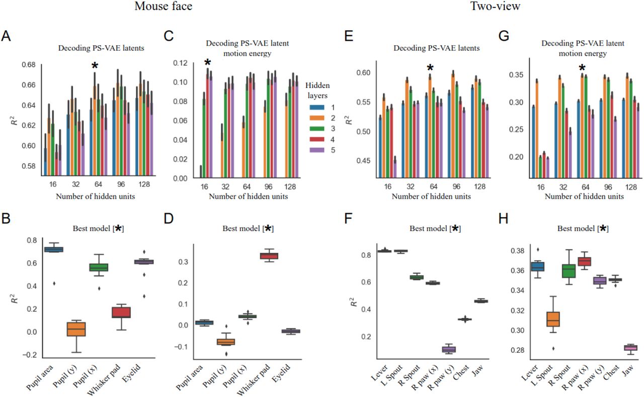
Results of hyperparameter searches for neural decoding models, which varied the number of hidden layers and number of hidden units per layer in a feed-forward neural network. A: Hyperparameter search results for decoding PS-VAE latents from the mouse face data. The “best” model is indicated with an asterisk (*), and is a chosen to balance model performance and model complexity. Error bars represent a 95% bootstrapped confidence interval over 10 random subsamples of 200 neurons. B: R2 results for the best model, separated by latent (same as Fig. 5C). The boxplot represents variability in R2 over the 10 random subsamples. C: Hyperparameter search results for decoding PS-VAE latent motion energy from the mouse face data. Error bars as in A. D: R2 results for the best model, separated by latent. Boxplot variability as in B. E-H: Same as A-D, except on the two-view dataset. Error bars represent a 95% bootstrapped confidence interval over test trials; boxplots represent variability across 10 bootstrapped samples from the test trials (see Methods for more information).

Comparison of neural decoding performance for the true labels (x-axis) and their corresponding supervised latents in the PS-VAE (y-axis), for both the mouse face dataset (panel A) and the two-view dataset (panel B); individual dots represent the median over test trials using different subsamples of neurons (panel A) or trials (panel B). The decoding accuracy is very similar across most labels in both datasets, indicating that the noise introduced in the PS-VAE label reconstruction does not have a large effect on the neural decoding of these quantities. The model architecture used for decoding the true labels is the same as the best model architecture found for decoding the PS-VAE latents.
6 Supplemental videos
The main figures in this work are accompanied by various videos demonstrating the performance of the PS-VAE and the downstream models. These videos include:
frame reconstruction ability of the PS-VAE (Fig. V1)
dynamic versions of the latent manipulations displayed in, for example, Fig. 2E-H (Fig. V2)
the various behavioral detectors obtained by training 2-state ARHMMs (Fig. V3)
neural decoding frame reconstructions (Fig. V4)
The following figures present a still from each of these video types, as well as links to each of the videos for each dataset presented in the paper.

Frame reconstruction video still. First (top) row: frames from the original behavioral video. Second row: reconstructed frames from the PS-VAE (left), residuals between these reconstructed frames and the original frames (center), and the corresponding PS-VAE latents (right). Colors are consistent with those in the main figures, and latent names are provided in the legend above. Third row: reconstructed frames from a standard VAE, the residuals, and the corresponding VAE latents. Fourth row: frames reconstructed from the labels only, without unsupervised latent dimensions (again with the residuals and the corresponding true labels). Reconstructions are shown for several batches of test data, which were not used for training or model selection. Each batch is separated by black frames in the reconstructed frames, and breaks in the traces.
6.1 Frame reconstruction video links
head-fixed mouse dataset: [link]
mouse face dataset: [link]
two-view dataset: [link]

Latent traversal video still. Each panel contains latent traversals for a single dimension, the name of which is indicated in the lower left corner of the panel. Supervised latents with associated labels use the label names; unsupervised latents that we have applied a post-hoc semantic label to are indicated with quotations, such as “Whisker pad” and “Eyelid” here. Unsupervised latents that have not been given labels (for example the VAE latents) are named Latent 0, Latent 1, etc. (none of this type are shown here). The supervised dimensions that correspond to 2D spatial locations contain an additional red dot that signifies the desired position of the body part, seen here in the Pupil (x) and Pupil (y) panels. The latent traversal procedure uses a base frame, indicated in the upper left corner of the figure. The videos show traversals for a range of base frames, and traversals for different base frames are separated by several black frames.
6.2 Latent traversal video links
head-fixed mouse
– PS-VAE [link]
– VAE: [link]
– Conditional VAE: [link]
mouse face
– PS-VAE: [link]
– VAE: [link]
– Conditional VAE: [link]
two-view
– PS-VAE: [link]
– PS-VAE (no paw tracking): [link]
– VAE: [link]
– Conditional VAE: [link]

ARHMM movement detector video still. Top: examples of video are played from 5 frames before to 5 frames after the transition from the still state to the moving state, as identified by the ARHMM. The state for each frame is indicated by the text in the bottom left corner. Different examples are separated by several black frames. Bottom: Corresponding traces of the PS-VAE latents used to fit the ARHMM; the latents corresponding to the current example are displayed in bold.
6.3 ARHMM detector video links
mouse face
– Saccade detector: [link]
– Whisker pad movement detector: [link]
two-view
– Body movement detector: [link]
– Paw movement detector: [link]
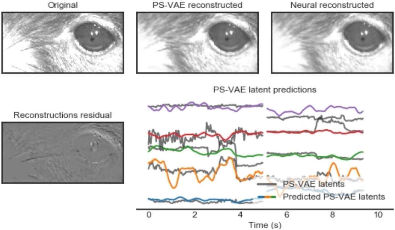
Neural decoding video still. Top left: frames from the original behavioral video. Top center: reconstructed frames from the PS-VAE. Top right: frames reconstructed by the neural activity. Bottom left: residual between the PS-VAE and neural reconstructions. Bottom right: PS-VAE latents (gray traces) and their predictions from neural activity (colored traces; colors are consistent with those in the main figures). Reconstructions are shown for several batches of test data, which were not used for the training or model selection of either the PS-VAE or the neural decoders. Each test batch is separated by black frames in the frame reconstructions, and breaks in the traces.
6.4 Neural decoding video links
mouse face: [link]
two-view: [link]
Acknowledgements
We thank Anne Churchland for helpful comments on the manuscript. We also thank the following for making their data publicly available: the International Brain Lab and the Angelaki Lab (head-fixed mouse), Matteo Carandini and Ken Harris (mouse face), and Simon Musall and Anne Churchland (two-view mouse).
Footnotes

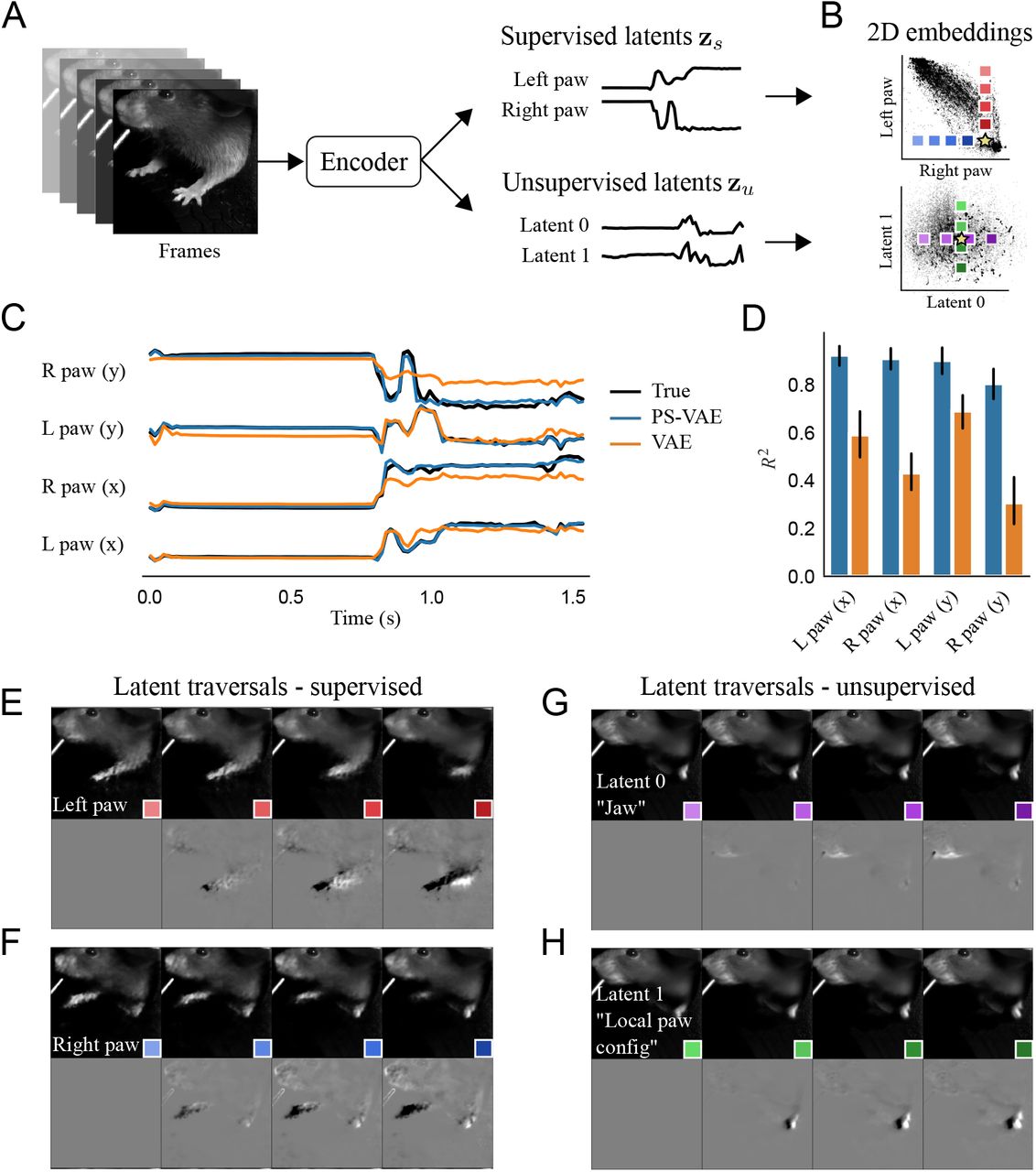
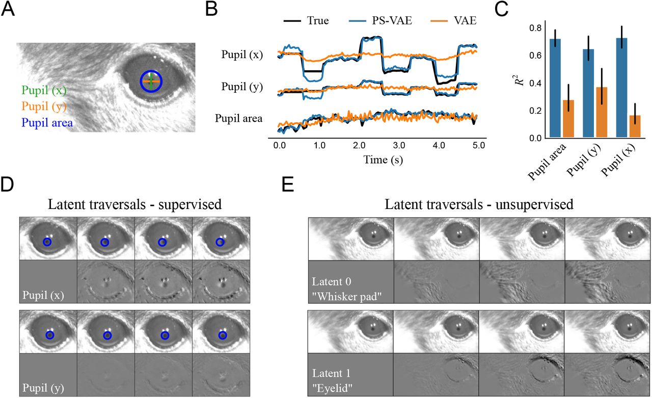
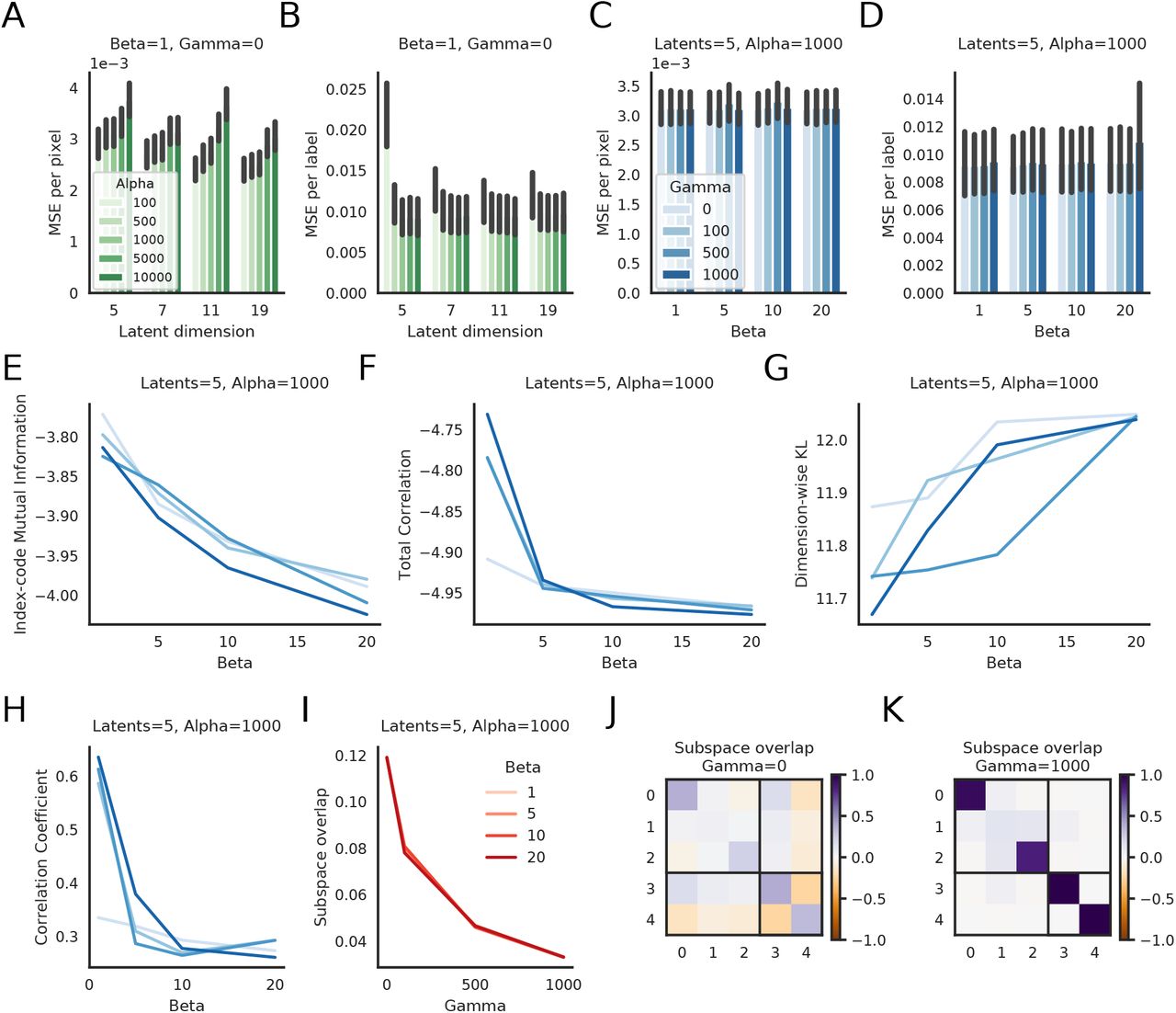
References
- [1].↵
- [2].↵
- [3].↵
- [4].↵
- [5].↵
- [6].↵
- [7].↵
- [8].↵
- [9].↵
- [10].↵
- [11].↵
- [12].↵
- [13].↵
- [14].↵
- [15].↵
- [16].↵
- [17].↵
- [18].↵
- [19].↵
- [20].↵
- [21].↵
- [22].↵
- [23].↵
- [24].↵
- [25].↵
- [26].↵
- [27].↵
- [28].↵
- [29].↵
- [30].↵
- [31].↵
- [32].↵
- [33].↵
- [34].↵
- [35].↵
- [36].↵
- [37].↵
- [38].↵
- [39].↵
- [40].
- [41].
- [42].↵
- [43].↵
- [44].↵
- [45].↵
- [46].↵
- [47].↵
- [48].
- [49].↵
- [50].↵
- [51].↵
- [52].↵
- [53].↵
- [54].↵
- [55].↵
- [56].↵
- [57].↵
- [58].↵
- [59].↵
- [60].↵
- [61].↵
- [62].↵
- [63].↵
- [64].↵
- [65].↵
- [66].↵
- [67].↵
- [68].↵
- [69].↵
- [70].↵
- [71].↵
- [72].↵
- [73].↵
- [74].↵
- [75].↵
- [76].↵
- [77].↵
- [78].↵
- [79].↵
- [80].↵
- [81].↵
- [82].↵
- [83].↵
- [84].↵
- [85].↵
- [86].↵
- [87].↵
- [88].↵
- [89].↵
- [90].↵
- [91].
- [92].↵
- [93].↵


