

Abstract
Predictive coding has been identified as a key aspect of computation and learning in cortical microcircuits. But we do not know how synaptic plasticity processes install and maintain predictive coding capabilites in these neural circuits. Predictions are inherently uncertain, and learning rules that aim at discriminating linearly separable classes of inputs – such as the perceptron learning rule – do not perform well if the goal is learning to predict. We show that experimental data on synaptic plasticity in apical dendrites of pyramidal cells support another learning rule that is suitable for learning to predict. More precisely, it enables a spike-based approximation to logistic regression, a well-known gold standard for probabilistic prediction. We also show that data-based interactions between apical dendrites support learning of predictions for more complex probability distributions than those that can be handled by single dendrites. The resulting learning theory for top-down inputs to pyramidal cells provides a normative framework for evaluating experimental data, and suggests further experiments for tracking the emergence of predictive coding through synaptic plasticity in apical dendrites.
1 Introduction
A hallmark of brain intelligence is its capability of using internal models, predictions, and internal goals that are maintained in higher brain areas to modulate, and arguably optimize, sensory processing in lower brain areas. This ubiquitous integration of context into sensory processing distinguishes brain computation from most other computing paradigms. Furthermore, we assume that the stereotypical laminar structure of cortical microcircuits supports this particular style of brain computation. In particular, inputs from higher brain areas preferentially arrive in pyramidal cells through synaptic connections in apical dendrites that are located in the upper layers of the laminar microcircuit. Hence in order to understand how context information from higher brain areas shapes sensory processing, we need to understand the plasticity mechanisms in apical dendrites of these pyramidal cells. One intriguing hypothesis is that pyramidal cells learn to predict bottom-up sensory inputs on the basis of information from other brain areas, including motor areas [Leinweber et al., 2017], that reaches these neurons through synapses on their apical dendrites [Xu et al., 2012, Larkum, 2013, Doron et al., 2020]. This hypothesis implies that plasticity of synapses at distal dendrites plays a key role for the emergence of predictive coding. Interestingly, a number of experimental data suggest that plasticity processes in apical dendrites differ in essential aspects from the more frequently studied correlative Hebbian or spike-timing-dependent plasticity (STDP)-like rules at other synaptic connections to pyramidal cells. In particular two differences have been emphasized: Firstly, the firing of the postsynaptic neurons, i.e., its somatic spikes, do not appear to play an essential role in the induction of this synaptic plasticity [Kampa et al., 2006, Kampa et al., 2007, Gambino et al., 2014]. Secondly, plasticity of these synapses is gated instead by other instructive signals [Magee and Grienberger, 2020], such as Ca2+-spikes [Kampa et al., 2006, Kampa et al., 2007], NMDAR spikes [Gambino et al., 2014], more general forms of plateau potentials within the dendritic arbor of pyramidal cells in area CA1 [Bittner et al., 2015, Bittner et al., 2017, Magee and Grienberger, 2020], or synaptic input from the perirhinal cortex [Doron et al., 2020]. These gating signals for synaptic plasticity have the common property that they are longer lasting events than postsynaptic spikes, extending over at least 50 ms. Hence we will refer to them as instructive signals in line with the terminology of [Magee and Grienberger, 2020].
In the case of Ca2+-spikes as instructive signals for synaptic plasticity, these Ca2+-spikes are typically generated when strong synaptic input to apical dendrites coincides with somatic spikes of a thick tufted pyramidal cell in layer 5. These somatic spikes may be caused by bottom-up sensory inputs, that arrive at synapses located below the dendritic tuft [Larkum, 2013]. Hence, prediction of Ca2+-spike can be seen for these neurons as a proxy for predicting sensory inputs.
A theoretical framework for analyzing these rules for synaptic plasticity at apical dendrites is missing, and a primary goal of this article is to establish such a framework. In addition, we propose a normative model for this form of synaptic plasticity. This normative model is based on the commonly conjectured learning goal for this synaptic plasticity: learning to predict. It takes into account that prediction is inherently uncertain, and can therefore not be learned well with learning rules such as the perceptron learning rule that is designed for learning classification of linearly separable classes of inputs. Furthermore, predictions are most useful if they are accompanied with an estimate of their uncertainty. For that one has to resort to models for learning probabilistic prediction, rather than classification.
We will first present a theoretical framework for learning probabilistic predictions through synaptic plasticity in a single dendritic branch in the apical tuft of a pyramidal cell, ignoring its interaction with other dendritic branches. We then extend the framework to the case where there are several dendritic branches in the apical tuft. There, we consider two types of experimentally reported interactions between dendritic branches, a saturating summation [Naud et al., 2014, Poirazi et al., 2003], as well as a soft XOR for pyramidal cells on layer 2/3 of the human cortex [Gidon et al., 2020]. We include illustrative examples for computational tasks that can be learned with the proposed model for synaptic plasticity in apical dendrites, both for the case of a single branch, and for the case of several interacting branches. For simplicity, we will refer to those dendritic branches in the apical tuft of pyramidal cells in layer 2/3 or 5, to which our learning theory applies, just as apical dendrites.
2 Results
2.1 A theoretically tractable model for prediction learning through synaptic plasticity in apical dendrites
We are considering a model for synaptic plasticity in apical dendrites that aims at being consistent with the main body of experimental data, and simultaneously at being as simple as possible so that it can be analyzed theoretically. Our model is closely related to the simple model for computations in apical dendrites of layer 5 pyramidal cells (L5Ps) proposed in [Larkum, 2013], see Fig. 1A. We have added to that a simple model for synaptic plasticity in these dendrites, see Fig. 1B.

A) Generic model of a thick tufted pyramidal cell in layer 5 of the stereotypical laminar cortical microcircuit, integrating two different inputs streams, see [Larkum, 2013] for details. A Ca2+-spike, which also propagates backwards into the dendritic tuft, is generated at the Ca2+-spike initiation zone when sufficiently strong depolarization arises from both input streams. This Ca2+-spike serves as the instructive signal in the sense of the plasticity model of [Magee and Grienberger, 2020] B) Illustration of synaptic input and output of the normative learning model, for the simplest case of a single dendritic branch. Synaptic input from neurons in higher brain areas with firing rates x1,…,xN is integrated with synaptic weights w1,…, wN in an apical dendrite. The normative learning model addresses plasticity of these weights, and the resulting depolarization qw(x) in the dendritic tuft represents the resulting prediction after learning.
The vector x = [x1, x2,…, xN]T represents the current firing rates of N neurons in higher brain areas that provide synaptic input to this dendritic branch. We write w = [w1, w2,…, wN]T for the synaptic weights of these synapses. We use the variable z to indicate the presence of a gating signal for synaptic plasticity, with z(t) = 1 if synaptic plasticity is enabled at time t, else z(t) = 0. This gating signal is referred to as the instructive signal in [Magee and Grienberger, 2020].
Since the analysis of synaptic plasticity in apical dendrites of these neurons [Kampa et al., 2006, Kampa et al., 2007] focused on the Ca2+-spike as a gating factor for synaptic plasticity in L5Ps, and since L5Ps are used as a running example for our analysis, we will refer in the following to this gating factor as a Ca2+-spike. But our analysis also holds if synaptic plasticity in apical dendrites is gated by a different signal, such as input from the perirhinal cortex according to [Doron et al., 2020], or a plateau potential in pyramidal cells of area CA1 that may emerge stochastically or triggered by attention or salience signals [Bittner et al., 2015, Bittner et al., 2017, Magee and Grienberger, 2020]. A common property of all these experimentally reported gating signals is that they last for 50 ms or longer.
We assume that the goal of synaptic plasticity of the weights w of synapses on the apical dendrite is the prediction of the gating signal z. Thus if this gating signal is triggered for example in pyramidal cells in layer 5 when the synaptic input from higher brain areas to the apical dendrites coincides with sensory inputs, this learning goal amounts to predicting coinciding sensory input to the neuron, see [Larkum, 2013]. Furthermore, we assume that the apical dendrites produce this prediction in the form of the depolarization qw(x) of the membrane potential that results from the current synaptic inputs x with weights w onto these dendrites. If one denotes the joint distribution of the input to the considered dendritic branch by x and the Ca2+-spike z by ptarget(x, z), then the optimal value of the model estimate qw(x) is the conditional probability ptarget (z|x). An important computational role of the resulting contribution qw(x) of distal dendrites to the processing of sensory information by a pyramidal cell in layer 5 was elucidated in [Takahashi et al., 2016] and [Takahashi et al., 2020]: it shifts the perceptual threshold.
Since Ca2+-spikes and the other gating signals that we are considering have a duration of 50 ms or more, we are looking for a synaptic plasticity rule which is consistent with this time scale, i.e., with a time scale that is slower than that of single spikes and EPSPs. In particular, we focus on a realization of the prediction qw(x) on this slower time scale: through the average membrane potential  that results from the firing rates x = [x1, x2,…, xN]T of neurons in higher brain areas that have formed synaptic connections on the considered apical dendrite. We approximate the resulting average membrane potential in this dendrite by:

It turns out that the resulting plasticity rule assumes a particularly simple form if one uses the following functional form for qw(x), which also takes into account a saturation effect:
 where
where  is the standard sigmoid function, u0 is a constant threshold, and β is a constant scaling factor.
In order to optimize qw(x) as approximation of ptarget(z|x), we use the cross entropy loss as a standard measure of the distance between the two distributions. A useful property of this loss function is that it is convex. Gradient descent for this loss function yields the following normative rule for synaptic plasticity of the weights w of synapses onto the apical dendrite:
 where Δwj is the change of the weight of synapse j and η > 0 is a constant scaling factor. We show in Section 3.2, that this weight update performs stochastic gradient descent for the previously described cross entropy loss. Because of the convexity of this loss function, this update is guaranteed to converge to its global optimum. Hence this plasticity rule is in a well-defined sense optimal, and this analysis provides the foundation for our normative model. The rule can equivalently be described in the form of Table 1. Note that it contains a weight decay term that is activated when the apical dendrite is depolarized, i.e., qw(x)) is large, but there is no gating signal, i.e., z(t) = 0. Both the LTP and the LTD component of the plasticity rule are proportional to the presynaptic firing rate xj.
The firing rates of presynaptic neurons in higher brain areas are denoted by x, and z is the gating signal. qw(x) is a function of the local dendritic membrane potential defined in equation 2.
Both the loss function that we minimize and the resulting type of plasticity rule are closely related to a well known optimization method in statistics and machine learning called Logistic Regression, see Methods. Hence we refer to the resulting synaptic plasticity rule as Dendritic Logistic Regression (DLR). For details regarding the implementation of this rule in simulations, see Methods.
2.1.1 A simple illustration of the capability of DLR to enable probabilistic predictions
Assume that there are two clusters of firing patterns x of neurons in higher brain areas that project to an apical dendrite of a pyramidal cell in layer 5, and that one can model each of these clusters by a Gaussian distribution  , with parameters (μ0, ∑0) and (μ1, ∑1). Furthermore, assume that firing patterns x from cluster k = 1 predict that a subsequent sensory input will arrive at the target neuron (thereby causing a Ca2+-spike in the neuron, i.e., a gating signal z = 1), and firing patterns from cluster k = 0 predict that this sensory input will not arrive (and that z = 0). Now assume that these two distributions overlap – as indicated by the clouds of dark green and light green dots in Fig. 2A. This occurs if many firing patterns x have significant probability under both of these distributions. In order to facilitate visualization, we consider here just two-dimensional firing patterns x, but the same principle applies for input patterns of arbitrary dimension. These two point clouds are not linearly separable, and hence the perceptron learning rule (as investigated in [Moldwin and Segev, 2020]) cannot do a good job of separating them, as indicated by the red trace in Fig. 2B. In contrast, synaptic weights in the apical dendrite can learn this inherently uncertain prediction task very fast through DLR; see the blowup of results for the first few trials in Fig. 2B. This large performance difference between perceptron learning and DLR might seem surprising. The perceptron learning rule is similar to the DLR given in equation 3, where qw(x) is replaced by qw(x) = 1 if
  and qw(x) = 0 if
  . The more fine-grained dependence of the DLR on the branch depolarization (equation 2) greatly improves the convergence properties. Moreover the apical dendrites learn through DLR to predict the probability that a spike input pattern x predicts a subsequent sensory input through the resulting value of qw(x) not only for those samples x that occurred during training, but they could generalize this probabilistic predictions to all potential values of presynaptic firing rates x. Furthermore the resulting predicting capability was on the same level as the theoretically optimal logistic regression learning rule, as shown in Fig. 2A. The resulting prediction capability through DLR can be measured through the negative log likelihood (NLL) in nats (lower is better) for the training data. Across a 100 independent training runs, it achieves an average of 0.378 nats, compared to 0.361 nats achieved through logistic regression.

A) Plot of probabilistic predictions for different firing rate patterns x of neurons in higher brain area that project to the considered apical dendrites, both as learned through DLR (at the top) and theoretically optimal predictions via logistic regression (below). The mean difference between the predicted probabilities is just 0.036. Also the resulting hyperplanes for resulting binary predictions for DLR and theoretically optimal logistic regression are very similar (bottom part). We also see a very rapid convergence of the DLR separation boundary after training with only 20 samples. B) Speed and accuracy of learning to guess (classify) from which cluster a presynaptic firing pattern x was drawn for the DLR learning rule and the perceptron learning rule, as considered in [Moldwin and Segev, 2020]. One sees that DLR enables much faster learning, and that the perceptron learning rule never converges to an optimal prediction performance. Mean and variance of the error are shown for 100 learning episodes with independently drawn initial weights and data points.
2.1.2 Predicting future sensory input caused by a moving object
Our brains are very good at estimating from the current position, speed, and movement direction of a moving object where this object will be at a later time point T. They can do this although estimates of movement speed and direction are inherently noisy, see the cartoon in Fig. 3B. We present a simple model which shows that this fundamental computational capability of neural circuits in the neocortex can be acquired through synaptic plasticity in apical dendrites. We assume that the receptive fields of a 2D array of neurons cover the movement field, and for simplicity, we represent the moving object by a linearly moving disk. The neurons in this array could for example be neurons in a visual or somatosensory area. We furthermore assume that these neurons receive from higher brain areas the estimated position, speed, and movement direction of a moving object at time 0, see Fig. 3A. We model the uncertainty of these estimates by adding Gaussian noise to an ideal estimate.
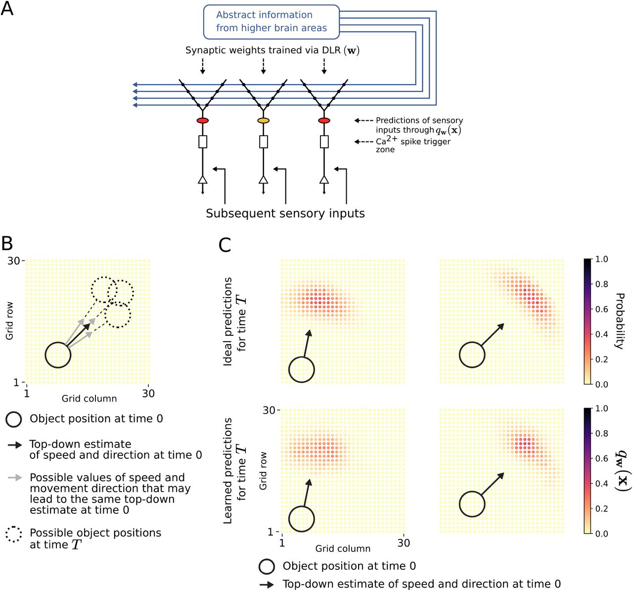
A) Schema of the simple network architecture that we consider. We assume that the position, speed, and movement direction of a moving object at time 0 are estimated in higher brain areas, and transmitted to the apical dendrites of a sheet of pyramidal cells, whose receptive fields cover the movement range by a 30 × 30 grid. More precisely, we assume that each of these neurons receives the same estimate. After learning, each apical tuft produces its individual probabilistic prediction, indicated by the same color code as used in panel C. B) For a particular top-down estimation of movement speed and direction, an illustration of three different possible trajectories of the moving object that may have resulted in this estimate. C) For two instances of this scenario we show in the lower row for each neuron in the 30 × 30 array its individual probabilistic prediction qw(x) that it generates in its apical dendrites, after self-supervised learning with DLR. Note that all these neurons receive the same synaptic input x in their apical dendrites. For comparison, we show in the upper row for each receptive field the actual probability that it will be covered at time T by the moving object, computed with knowledge of the full distribution of noisy estimates for time 0.
During learning, the neurons in this 2D array receive at time T both, these estimates from higher brain areas that arrive at their apical dendrites, and whether the receptive field of the neuron is covered at this time T by the moving object, as strong sensory inputs on their basal dendrites. We assume that the coincidence of both signals causes a Ca2+-spike, thereby triggering in the apical dendrites of the neuron synaptic plasticity via DLR. We show in Fig. 3C that the neurons learn in this way to predict through the membrane potential qw(x) generated by synaptic inputs x to their apical dendrites whether their receptive field will be covered at time T by the moving object. This holds whenever the input x to their apical contains the estimates of movement speed and direction at time 0. Hence when these estimates are provided before time T, the apical dendrites will produce a probabilistic prediction of a future event. These learnt predictions are shown in the lower row of Fig. 3C for two different movement scenarios. A comparison with the probabilistic ground truth in the upper row of Fig. 3C shows that the learnt probabilistic movement predictions are close to optimal. Note that the probabilistic ground truth in the upper row was computed on the basis of full knowledge of the distribution of the noisy estimates of speed and direction at time 0.
2.2 Extensions to the case of multiple dendritic branches
When there are several dendritic branches, the question arises as to how the contributions from different branches are combined for the prediction qw(x). Here, we denote the weights and inputs into each dendritic branch B by  and
and  respectively, and the weights and inputs across all branches as w, x respectively. We denote the predicted distribution by qw(x) (similarly to equation 2), which estimates the target conditional distribution ptarget(z = 1|x).
It was shown in [Naud et al., 2014] that a neuron model with a somatic and dendritic compartment can accurately predict spike responses of cortical pyramidal neurons. Similar two-layer models have been proposed for hippocampal CA1 pyramidal cells [Poirazi et al., 2003] and even for cortical interneurons [Tzilivaki et al., 2019]. In general, it is believed that two-layer models provide a viable model for neocortical and hippocampal pyramidal cells [Jadi et al., 2014]. In this model the activity of each dendritic branch saturates according to a sigmoidal nonlinearity. Dendritic outputs are then summed and another non-linearity is applied to model the neuron output activity. In line with this model, we assume that the contributions from each dendritic branch (fB) are a function of the mean branch local membrane potential  (equation 1) and consider a model of qw(x) that accumulates contributions from the dendritic branches:

Consistent with the single-branch model (equation 2), the contribution of each branch is given by a sigmoidal function of its weighted input rate, i.e.

For the function ψ we consider two possibilities. According to the classical two-layer model, the neuron output activity is given by a saturating nonlinearity applied to the summed dendritic contributions. Hence, as a first possibility, we model ψ as a sigmoidal function in Subsection 2.2.1 below. More recently, a more complex relationship was found for single human neurons [Gidon et al., 2020] which will be considered in Subsection 2.2.2.
2.2.1 Saturating model
In the first possibility, taking into consideration the thresholding and saturation dynamics of pyramidal neurons [Naud et al., 2014, Jadi et al., 2014], we chose the sigmoidal shape for ψ to get
 where α and ϑ are suitable constants. Note that by choice of α and ϑ, one can model different types of (soft-) logic operations. A low ϑ lesser than 1 implements a soft OR operation (a minimum of one branch needs to be active to get a high probability output). A ϑ close to the number of branches implements a soft AND, and in-between we obtain a general threshold condition on the number of active branches. See Fig. 4B (left and middle) for an example with two branches.

A) We consider here for simplicity the case of two branches of the dendritic tuft that both receive synaptic input from the same two neurons in a higher brain area, for two experimentally reported types of interaction of their contributions: saturating and soft-XOR. B) The resulting probabilistic predictions ψ(ftotal) of the apical tuft are shown after training on three different datasets. Note that for neither one of these datasets a single-branch probabilistic prediction as shown in Fig. 2 suffices. But both experimentally observed saturating and XOR-like interactions between different dendritic branches enable DLR to produce suitable distributions of probabilities, indicated again through color coding, that separate the two point clouds. Note that like in the case of Fig. 2, a number of these training examples could have been generated by either one of the two distributions that generate dark green and light green datapoints. Hence probabilistic predictions are needed, like in the case of Fig. 2. But with DLR running in parallel in several apical dendrites, also complex distributions of datapoints can be handled (Table 2).
The goal of the learning rule in this case is to get qw(x) to predict the probability ptarget(z = 1|x) of Ca2+-spikes that occurs during training. Hence a normative model for synaptic plasticity in these dendritic branches should minimize the distance between these two terms, formulated again as cross-entropy error.
The above choices for fB and ψ lead to the following weight update rule for the incoming weights to a particular dendritic branch B:
 where η is a learning rate and
  is the derivative of fB. This update is similar to the single-dendrite update, with two differences: (1) the term
  means that there is a nonlinear dependence on the local branch potential, and (2) the update depends on ψ (ftotal). This quantity is not local to the dendritic branch. In order to minimize the information about ψ (ftotal) at the branch, one can consider a gating of updates based on thresholds on ψ (ftotal) which approximates the term (z – ψ (ftotal)) in the update rule 7. This leads to the following updates of synaptic efficacies:
 for plasticity thresholds q− and q+. To see the correspondence with rule 7, first consider the case without Ca2+-spike (z = 0). Here, the term (z – ψ (ftotal)) in equation 7 is between –1 and 0. It becomes very small when ψ (ftotal) is close to zero. This is approximated by a gating mechanism which blocks plasticity if ψ (ftotal) is below some threshold q− close to 0. When there is a Cabspike (z = 1), the term (z – ψ (ftotal)) is between 0 and 1. It becomes very small when ψ (ftotal) is close to one. Hence, plasticity is blocked if ψ (ftotal) is above some threshold q+ close to 1 in the approximation 8.
2.2.2 Soft-XOR model
This second choice for ψ is motivated by recent findings from human L2/3 pyramidal cells. According to [Gidon et al., 2020], Ca2+-spikes are initiated in these cells at a threshold activation ϑ of dendrites, but if dendrites are even more strongly activated, these spikes are not elicited. We can model such behavior by a nonlinearity ψ(ftotal) that is close to 1 in a certain activation region (ϑ, ϑ + Δϑ), see Fig. 4B (right) and Methods.
A plasticity rule for this model is derived in Methods, where the plasticity at the synapse depends on ftotal. Again, we can consider a coarse influence of ftotal on the local plasticity, where it switches between LTP, LTD, and no update based on three thresholds f− (low ftotal), fmid (medium ftotal), and f+ (high ftotal), see Fig. 4B (right). This leads to the following updates of synaptic efficacies:

We can interpret these plasticity dynamics as follows. Assume first the case of a Ca2+-spike z = 1. For low ftotal (< f−), the activation has to increase in order to increase the probability of the model. Hence active synapses are potentiated. For medium ftotal (f− ≤ ftotal ≤ f+), we have already a high probability for a Ca2+-spike. Hence, no update is necessary. For high ftotal (> f+), the activation is too high and depression is needed. Consider now the case of no Ca2+-spike z = 0. If the neuron is at medium ftotal, the probability can be decreased either by decreasing the activation (LTD) or increasing it (LTP). In the upper half of the “high probability bump” (fmid < ftotal ≤ f+), LTP is chosen, and in the lower half (f− ≤ ftotal < fmid) LTD is chosen, which shift ftotal in the direction leading to a decreased probability. Outside of this, i.e. for ftotal > f+ and ftotal < f−, we already predict a low probability of Ca2+-spike and thus no updates are necessary.
2.2.3 Demonstration of the enhanced probabilistic prediction capabilities that emerge through DLR in the case of several apical dendrites
Similar to as shown in Fig. 2 we assume here that data points with labels z = 0 or 1 are drawn from some overlapping probability distributions. But in contrast to Fig. 2 we assume here that these distributions are not just Gaussians that can be separated by an optimal linear decision boundary. Examples for the resulting clouds of data points are shown for three examples of more complex distributions in Fig. 4B.
Using a model with two dendritic branches, we consider three different kinds of interactions between these two branches – a saturating interaction with a low threshold, high threshold, and a soft-XOR interaction. One sees in Fig. 4B that each of these three types of interactions is useful for learning probabilistic predictions for three different types of distributions of data points. Furthermore one sees that training via DLR enables the dendritic branches to also provide meaningful predictions for presynaptic firing rates x that never occurred during training.
A detailed quantitative evaluation is provided in Methods, see Table 2 there. Here we summarize these results: When using two dendritic branches, the cases of saturating interaction with low and high value of the strong spike threshold perform very well on the OR and AND tasks respectively. The Soft-XOR interaction performs much better than the saturating interaction in modelling the XOR dataset. This validates the intuitive understanding of the different interactions and how they correspond to different Boolean operations. Adding more branches with a saturating interaction with an intermediate threshold value ϑ, we see that these configurations perform very well across all the three datasets thus showing that increasingly complex distributions can be modelled by a single configuration given enough branches.
Mean negative log likelihood (NLL) in nats (lower is better) is given for the training sets of the three different data distributions considered in 4B, and for the three types of interactions among apical dendrites that we consider, as well as for different numbers of apical dendrites. One sees that using a saturating interaction with low threshold for two branches excels at the OR task, while the high threshold scheme excels at the AND task. The Soft-XOR interaction turns out to be substantially more effective for learning with two branches the probabilistic prediction for the case of the XOR data distribution. However, with more branches the saturating interaction supports learning of probabilistic predictions via DLR for all three tasks. Each of the mean NLL values above is calculated from the best 8 out of 14 independent training runs (to avoid outliers which do not converge).
3 Methods
3.1 Implementation Details of DLR
Each dendritic branch indexed by B receives top-down input xB weighted by input weights wB. An input vector  is presented to the branch as input spike trains
  for a fixed duration. Mathematically, we model the spike trains
  as sums of Dirac delta pulses at spike times. For each n, the spike times are generated by a Poisson point process of rate equal to
  .
.
For the duration of the input presentation, the membrane potential u is given by the weighted sum of the spike trains convolved temporally with a linear postsynaptic potential kernel kPSP
 where we use a double exponential PSP kernel

In our simulations, we used values λPSP = 1, τf = 2 ms, and τr = 10 ms for the scaling- and time-constants.
We define the quantity  as the un-weighted contribution of incoming synapse n to the dendritic potential in branch B. For any PSP shape, the expectation of
  is proportional to the spike input rate
  .
.
Thus, for the weight update rule in 3, we use the time average of the membrane potential  to calculate qw(x), and the time average of
  in lieu of
  . This is because
  is a quantity that is local to the incoming dendritic synapse and can thus be used in local synaptic weight updates.
For the case of the single branch SLR, the implemented weight update is thus given by
 where we make use of the definition of qw(x) from equation 2.
For the multi-branch update rules, we use  and
and  in lieu of
  and
and  respectively when implementing the weight update rules corresponding to the saturating and soft-XOR dynamics in equations 8, 9.
3.2 Derivation of DLR for a single branch
In general, each dendritic branch indexed by B receives top-down input xB weighted by weights wB. Here, we consider the case of a single dendritic branch. Hence, to simplify notation, we will in the following suppress the superscripts and simply write x for the inputs to this branch and w for the corresponding weights. In our model the input x represents the vector of firing rates of the neurons presynaptic to the dendritic branch.
The Ca2+-spikes are denoted by z where z = 1 denotes the presence of the calcium spike, and z = 0 denotes the absence of a Ca2+-spike for the duration of the input. We denote the joint distribution of the input x and the calcium spikes z as ptarget(x,z). Our regression formulation then seeks to provide an estimator parametrized by w (qw(x)) which is optimized to approximate ptarget(z = 1|x). Namely, we aim to train the weights w so that qw(x) accurately predicts the probability of the occurrence of a Ca2+-spike given a particular top-down input x.
The cross entropy loss function that measures the distance between qw(x) and the data distribution ptarget is defined by
 where x, z are sampled from the data distribution ptarget.
The corresponding gradient with respect to the parameters w is given by

In our case, we take into account the fact that qw(x) is a function of the dendritic membrane potential which is proportional to wTx. Hence, if qw(x) takes the simple form q(wTx) for some nonlinearity q, one gets

A further simplification arises if one uses a logistic sigmoid function as nonlinearity q such that:
 where
where  and β and u0 are model constants. Hence, in this case, the predictive depolarization that results from synaptic currents at the dendrite is a saturated version of
  as given in equation 2. Then, using the fact that σ′(α) = σ(α) (1 – σ(α)), one obtains

When we insert the definition of qw(x) from equation 15 into the loss function  , we find that this loss function corresponds to a well known linear regression scheme called Logistic Regression. It is known that this loss function is a convex loss function.
Thus, with x encoded as the mean input spike rate, and  (equation 1), we see that the weight update rule described in equation 3 performs stochastic descent along the gradient of the convex logistic cross entropy loss function. This guarantees the convergence of the weight update to the global optimum of the loss function.
3.3 Derivation of DLR for the case of multiple branches
Here, xB, wB represent the weights and input to dendritic branch B, and x, w represent the full input and weights. The corresponding cross entropy loss with qw(x) defined as in equation 4 is given by

The derivative of the above loss with respect to the weights wB of a branch B evaluates to

3.3.1 Derivation of DLR for the saturating model
In this model, a sigmoidal shape for ψ is chosen:
 where α and θ are suitable constants. Using this in equation 18 we obtain the gradient for the saturating model:
 which leads to the weight update rule in equation 7.
In order to minimize the information about ψ (ftotal) at the branch, one can consider a gating of updates based on thresholds on ψ (ftotal) which approximates the term (z – ψ (ftotal)) in the update rule 7. We consider the two cases z = 0 and z = 1 separately. For z = 0, the term (z – ψ (ftotal)) is between –1 and 0. It becomes very small when ψ (ftotal) is close to zero. A gating mechanism which blocks plasticity if ψ (ftotal) is below some threshold q− close to 0 approximates this term. For z = 1, the term (z – ψ (ftotal)) is between 0 and 1. It becomes very small when ψ (ftotal) is close to one. A gating mechanism which blocks plasticity if ψ (ftotal) is above some threshold q+ close to 1 approximates this term. Hence, we can formulate the approximate update 8.
3.3.2 Derivation of DLR for the soft-XOR model
In the soft-XOR model, ψ is given by


Suitable parameters α, θ, and Δθ lead to an XOR-like behavior (high probability in a certain activation region), see Fig. 4B (right). Using this nonlinearity in equation 18, we obtain

Considering a coarse influence of the ftotal on the local plasticity, we can formulate an approximate rule which switches between LTP, LTD, and no update based on three thresholds f− (close to ϑ), fmid (ϑ + Δϑ/2), and f+ (close to ϑ + Δϑ), see Fig. 4B. This leads to the updates given in equation 9.
3.4 Simulation Details: Classification of 2D data (Fig. 2)
The training examples for this task consist of points generated from two 2D Gaussian clusters with means and covariances μk, ∑k for k ∈ {0,1}. All points generated from  have the target value z = k. The prior probabilities for the classes 0 and 1 were chosen to be equal (0.5). Thus to generate a training sample (xi, zi), we first pick the Gaussian component k ∈ {0,1} with equal probability i.e. k ~ bernoulli(p = 0.5). We then pick
  and assign the target zi = k. This gives the following conditional probability distribution p(z = 1|x)
 where p(x|k) is the Gaussian probability density function with mean μk and covariance ∑k. It is the aim of the algorithm to learn this conditional distribution in the quantity qw(x) in the dendrite (equation 2).
The covariance matrix ∑k can be decomposed as  . Here Vk is an orthogonal matrix where the columns are the eigenvectors of ∑k and give the directions along which the 2D Gaussian is aligned. Sk is a diagonal matrix with each diagonal entry representing the standard deviation of the Gaussian along the corresponding eigenvector. The parameters used for this simulation are:

For this demonstrative simulation we consider the neuron to be receiving the input on a single dendritic branch, with the DLR being applied to the incoming weights to that branch. Each data point xi, is padded with an additional component of constant rate of 40Hz (in order to model intercept fitting). Each component of this data point is then given as input to the network encoded as a Poisson spike train with mean rate equal to the value of the component. This spike train is provided to the neuron for a duration of 400 ms. Targets are fed to the network by enabling or disabling Ca2+-spike firing corresponding to z = 1 and z = 0 respectively. Fig. 1B illustrates this neuron and learning setup.
When training the input weights to the neuron using DLR, the initial weights for each run are initialized to positive values drawn from a normal distribution with mean 9.0 and standard deviation 4.5. The weights are clipped at zero so that they stay positive in order to obey Dale’s law.
The standard perceptron classifier trains a set of weights w so that for any data point (x, z), we should have wTx > 0 if z = 1 and wTx < 0 if z = 0. For each iteration of updating the weights w, we randomly sample a single data point (x, z) from the target distribution ptarget, and apply the following standard perceptron update to weights w. Note that we also add here the same additional component of 40Hz to x to enable the perceptron to train the intercept of the separating line.

The learning rates η for both the DLR and perceptron learning (used in equations 3, and 24 respectively) decay harmonically from an initial value of η0 to a final value of ηfinal over the course of the 30000 iterations that we run them for in Fig. 2. For the DLR we use η0 = 1.8 (See Table 3), and for the perceptron learning we use η0 = 0.01, where the lower learning rate is used to aid any possible convergence of the perceptron. In both cases ηfinal = η0/6. Thus we see that even with a lower learning rate and an idealized perceptron learning, the perceptron rule does not converge for this case where the data is not linearly separable.
Parameters related to DLR that are used for each experiment. η0, ηfinal are the initial and final learning rate used. β and u0 are the scale and threshold for the sigmoid function used to calculate qw(x) and fB in equations 2 and 5 respectively.
3.5 Simulation Details: Predicting the future sensory input from a moving object (Fig. 3)
3.5.1 Input encoding and parameters
In our simulation, the moving object is a 2D circle which moves within a 30 × 30 grid and has a diameter of 5 Grid Units (GU). We consider here the task of predicting the sensory input corresponding to its position after a fixed delay of T. The top-down input corresponding to an instance of a moving object is specified by a four-tuple (rx, ry, v, θ) consisting of x and y coordinates rx, ry of the initial position, the speed v, and the direction angle θ. This four-tuple is encoded in a population coded manner described below. This set of population coded inputs is connected to a 30 × 30 grid of L5P neurons (one neuron per grid position). The speed and direction are perturbed by a Gaussian noise to model inaccuracies in top-down measurement. This grid is trained to reproduce the image of the ball at its final position which is determined by the initial position and the true (unperturbed) velocity in the external environment. The incoming weights to each L5P neuron are trained using DLR with the target being the corresponding pixel value in this image.
The top-down inputs specifying the initial position and velocity of the ball are encoded as follows. The initial position (rx, ry) can take any value such that both rx, ry take values in the range of Sr = [3,27] GU. The speed v is defined in terms of the distance (in GU) that the moving object covers in the fixed delay T between the top-down and the bottom up inputs. This distance can take any value in the range Sv = [4,20] GU. The direction is specified by an angle θ to the horizontal which can take any value in the range [0, 2π).
In addition, before being given as input, the speed v and the direction angle θ are perturbed by the addition of a Gaussian noise in order to model a noisy estimate of the object velocity. This means that given a particular initial position and velocity as input, the true velocity of the ball and consequently the final position of the ball is uncertain.
The encoding of these values into neuron populations is described below. We consider the sets Mr, Mv and Mθ, which consist of Nr, Nv, and Nθ equally spaced values in the ranges Sr, Sv, and Sθ respectively. Then, corresponding to each four-tuple (μx, μy, μv, μθ) ∈ Mr × Mr × Mv × Mθ, we have a single input neuron that fires according; to a Gaussian tuning curve centered at (μx, μy, μv, μθ). The neuron encodes the input (rx, ry, v, θ) by firing at a rate ρ given by
 where Z is a normalization factor calculated so that the total spike rate of all the input neurons is ρtotal = 250 Hz. Here the standard deviation of the response curve corresponding to position σr, velocity σv, and direction σθ are constant across all neurons.
For the simulation whose results are shown in Fig. 3, we use Nr = 10, Nv = 10, Nθ = 24, σr = 2.67, σv = 1.78, σθ = 0.2618 = 15.0°. This leads to a total input dimension of Nr2NvNθ = 24000. The standard deviations of the Gaussian noise perturbations applied to the speed and direction components of the top-down input are equal to the width of the respective receptive fields σv, σθ. In order to train the network we make use of 168000 data points in the training dataset.
All the weights are initialized to a constant positive value of 9.0 and are clipped at zero during training so that they stay non-negative in accordance with Dale’s law.
3.5.2 Calculating actual probability of a neuron’s receptive field being covered by the object at time T
The imprecision in the estimate of the object velocity, modeled by the perturbed input speed and direction, leads to the final position of the object being uncertain. Each pyramidal neuron in the 30 × 30 grid receives as input to the apical dendrites the four-tuple sin ≜ (rx, ry, vin, θin). Here (rx, ry) is the initial position of the object and (vin, θin) are the noisy estimates of speed and direction of the velocity used by the pyramidal neuron. We denote the true velocity of the object by (v, θ), and define the corresponding four-tuple s ≜ (rx, ry, v, θ).
Consider a single neuron in the grid. For this neuron, we denote as Z the random variable such that Z = 1 if and only if the object covers the receptive field of this neuron at time T, and Z = 0 otherwise. Given the noise in the estimate of velocity, we thus wish to calculate p(Z = 1|sin), which is the conditional distribution that is estimated by the neuron via qw(x)

Here we use the fact that the final position of the object is fully determined given the true velocity and the initial position s.
To calculate p(s|sin) we use the following facts regarding (v, θ) and (vin, θin) (as in description of input above)

Thus, using Bayes’ theorem, we can calculate

The above can be computed using the fact that p(sin|s) is the probability density function of a normal distribution.
3.5.3 Measurement of performance
Here we provide measurements to demonstrate that the network reliably predicts the probability that a neuron receives input from the moving object at time T. We term the position of the center of the moving object as predicted by the noisy estimate of the velocity as the estimated final position. We then consider three concentric slices of the neuron grid centered at the estimated final position, with diameters 0 – 5 GU, 5 – 9 GU, and 9 – 13 GU. For the pyramidal neurons within a slice, we compare the mean predicted probability qw(x) and the mean actual probability, of their receptive fields being covered by the object at time T.
Slice of diameter 0 – 5 GU: mean qw(x) = 0.3546, mean actual probability = 0.4108
Slice of diameter 5 – 9 GU: mean qw(x) = 0.1666, mean actual probability = 0.1668
Slice of diameter 9 – 13 GU: mean qw(x) = 0.0461, mean actual probability = 0.0435
From this we can clearly see that the mean predicted probability qw(x) drops away from the estimated final position, as well as that the theoretically calculated probabilities are followed closely by the predicted probabilities. The examples in Fig. 3 and the results above are calculated from combinations of initial position and velocity that were not seen during training.
3.6 Simulation Details: Predicting complex distributions with multiple dendritic branches (Fig. 4)
In this experiment, the 2D data is generated from multiple gaussian clusters. The parameters and the class labels assigned to each cluster are chosen to create datasets corresponding to an OR, AND, and XOR operation shown in Fig. 4.
In order to solve this task, we consider a neuron with NB (two or more) dendritic branches each with their respective incoming synapses with weights w1,…, wNB. All of these branches receive the same 2D input, i.e., xB = [x; 1] = [x1, x2,1] for B = 1,…, NB. This input is provided as in the 2D regression task for a single branch, i.e., as a spike sequence with a spike rate proportional to the input value. The additional input component with a value of 20 Hz is given in order to model the training of the branch baseline activation.
The various configurations in table 2 along with corresponding parameters are below.
2 Branches, saturating interaction, low threshold ϑ = 0.6: This implements the OR operation between the two branches.
2 Branches, saturating interaction, high threshold ϑ = 1.2: This implements the AND operation between the two branches.
2 Branches, soft-XOR interaction, ϑ = 0.5, Δϑ = 1.0. This implements the XOR operation between the two branches.
4 Branches, saturating interaction, ϑ = 1.4.
6 Branches, saturating interaction, ϑ = 2.1.
For all the saturating interactions, we use a scale factor α = 12. The parameters q+, q− used in the learning rule in 8 are set to q+ = 0.9 and q− = 0.1. For the Soft-XOR interaction, we use α = 8.0 and set f− = ϑ = 0.5, f+ = ϑ + Δϑ = 1.5 and fmid = ϑ + Δϑ/2 = 1.0.
The initial weights for each branch B are initialized in the following manner. We pick a point  , where both
  are randomly picked uniformly from the interval [110,130] Hz. We then pick a random direction vector hB sampled uniformly from a unit circle. Using this pair of sB,hB, we set the initial weights
  so that the separating plane is a plane that passes through the point sB, with the direction of the plane determined by the normal vector hB. The weights in this case are unconstrained in sign to allow the model to fit the complex distributions in the case of the low dimensional inputs.
3.7 Common Parameters for DLR
Some of the common parameters and the values for the DLR rule for the three experiments are given in Table 3.
4 Discussion
We have presented a mathematical framework and learning theory for the arguably most important synaptic connection for the integration of top-down predictions from higher brain areas into computational processing of sensory input in lower areas: Synapses from axons of neurons in higher brain areas onto apical dendrites of pyramidal cells in lower areas. Experimental data show that plasticity at these synapses follows rules that differ from rules for correlated Hebbian learning, because they are gated by instructive signals [Magee and Grienberger, 2020]. Furthermore these instructive signals differ from commonly considered global third factors for synaptic plasticity, such as dopamine, that typically signal reward. Instead, these instructive signals either emerge locally within the neuron — such as Cabspikes [Kampa et al., 2006, Kampa et al., 2007], NMDAR spikes [Gambino et al., 2014], or other types of plateau potentials [Bittner et al., 2015, Bittner et al., 2017, Magee and Grienberger, 2020] – or arrive in the dendritic tuft through synaptic connections from brain areas such as the perirhinal cortex [Doron et al., 2020] or higher order thalamus [Aru et al., 2020]. We have focused in our illustrative example in Fig. 1 and in the text on the case where these instructive signals, denoted by z in our mathematical models, take the form of Ca2+-spikes. But our theoretical framework and normative learning theory also applies to other forms of instructive signals. The only aspect on which this learning theory is based is that these instructive signals last for 50-100 ms or longer, so that the firing rates of presynaptic neurons become salient, rather than single spikes.
Apart from these neurophysiological differences, the functional impact of plasticity at these synapses on apical dendrites has been shown to differ from that of other synaptic connections. For example, the input from apical dendrites has been shown to shift the perceptual threshold in a graded manner [Takahashi et al., 2016]. In addition, if these synapses learn to predict sensory inputs on the basis of inputs from higher brain areas, such predictions are inherently uncertain, and therefore would be functionally most useful if they aim at learning probabilities, rather than categorical decisions. We have shown that this learning goal can be achieved through simple rules for LTP and LTD, gated by instructive signals z, at synapses on apical dendrites. In fact, a suitable balancing of LTP and LTD can produce a depolarization of the dendritic tuft that approximates logistic regression, i.e., a simple form of probabilistic prediction that is in a well-defined sense optimal. Hence we refer to this normative model for synaptic plasticity in the dendritic tuft as dendritic logistic regression (DLR). We have shown in illustrative examples that DLR enables the dendritic tuft to make meaningful probabilistic predictions in the case where the same prediction is sometimes correct and sometimes not (Fig. 2A). Furthermore these probabilistic predictions can be learnt really fast through DLR (Fig. 2B). In particular, they provide substantially better performance than the perceptron learning rule [Moldwin and Segev, 2020]. The reason is that the latter is guaranteed to work well only if the training examples are linearly separable, in particular if they do not contain contradicting examples that commonly occur in the case of probabilistic predictions. We have also demonstrated in Fig. 3 that the DLR rule enables distal dendrites to predict future sensory inputs caused by a moving object.
A concrete experimentally testable prediction of this normative model is that, after learning, the depolarization in a dendritic branch of the tuft is correlated with the probability that the current synaptic input to the dendritic tuft coincides with an instructive signal, for example with a Ca2+-spike. Another experimentally testable prediction of our model is that the current depolarization of the dendritic branch scales the amplitude of LTP and LTD during the induction of plasticity. In particular, if synaptic input to an apical dendrite coincides with a plateau potential, the expression of LTP is predicted to be weaker if the dendrite is already strongly depolarized. Furthermore, our normative model predicts that synaptic input to an apical dendrite causes LTD in the absence of a plateau potential, and the impact of LTD is stronger if the apical dendrite is already stronger depolarized. Our model also raises the question whether LTP of synapses on distal dendrites of pyramidal cells in other brain areas besides the neocortex, such as area CA1 [Bittner et al., 2015, Bittner et al., 2017], is also accompanied by a corresponding forms of LTD, and whether LTP and LTD combine to generate probabilistic predictions of other events.
We have extended our learning theory in the second part to the case of several interacting branches in the dendritic tuft. Two different types of interactions have been found in experiments: Summation of depolarization [Jadi et al., 2014, Poirazi et al., 2003], and competition between depolarized branches [Gidon et al., 2020]. We have characterized in Fig. 4 additional capabilities of probabilistic prediction that are enabled by DLR for these two types of interactions between dendritic branches. In both cases, probabilistic predictions emerge that can learn predictions for substantially more complex distributions than for the simplified case of a single dendritic branch. In this sense, our learning theory also throws new light on likely computational contributions of the dendritic arbor.
Acknowledgments
This work was supported by the European Union’s Horizon 2020 Framework Programme for Research and Innovation under the Specific Grant Agreements No. 785907 (Human Brain Project) and No. 899265 (ADOPD).
Footnotes
↵* First authors
The results corresponding to the prediction of the moving object have been clarified to show how the target distributions are accurately predicted. Figure 3 has been correspondingly revised. The methods sections have been updated to include missing parameters and to specify the precise implementation of the learning rule using input spikes. Title has been changed.
References
- [Aru et al., 2020].↵
- [Bittner et al., 2015].↵
- [Bittner et al., 2017].↵
- [Doron et al., 2020].↵
- [Gambino et al., 2014].↵
- [Gidon et al., 2020].↵
- [Jadi et al., 2014].↵
- [Kampa et al., 2006].↵
- [Kampa et al., 2007].↵
- [Larkum, 2013].↵
- [Leinweber et al., 2017].↵
- [Magee and Grienberger, 2020].↵
- [Moldwin and Segev, 2020].↵
- [Naud et al., 2014].↵
- [Poirazi et al., 2003].↵
- [Takahashi et al., 2020].↵
- [Takahashi et al., 2016].↵
- [Tzilivaki et al., 2019].↵
- [Xu et al., 2012].↵


