

Abstract
Motivation Gene co-expression analysis is an attractive tool for leveraging enormous amounts of public RNA-seq datasets for the prediction of gene functions and regulatory mechanisms. However, the optimal data processing steps for obtaining high-quality co-expression networks from such large datasets remain unclear. Especially the importance of batch effect correction is understudied.
Results We conducted a systematic analysis of 50 different data processing workflows and applied them on RNA-seq data of 68 human and 76 mouse cell types and tissues. We analyzed the resulting 7,200 gene co-expression networks and identified the factors that contribute to their quality focusing on data normalization, batch effect correction and the measure of correlation. We confirmed the key importance of large sample counts for generating high-quality networks. However, choosing a suitable normalization approach and applying batch effect correction can further improve the quality of co-expression networks, equivalent to a >70% and >40% increase in samples count. Finally, Pearson correlation appears more suitable than Spearman correlation, except for smaller datasets.
Conclusion A key point in constructing high-quality gene co-expression networks is the collection of many samples. However, paying attention to data normalization, batch effects, and the measure of correlation can significantly improve the quality of co-expression estimates.
Introduction
Understanding the functions and regulatory mechanisms of genes is one of the central challenges of biology. Gene co-expression is an important concept in bioinformatics because it serves as a foundation for predicting gene functions and regulatory mechanisms, for more complex network inference methods, and for gene prioritization (Eisen et al., 1998; Wolfe et al., 2005; Zhang and Horvath, 2005; Usadel et al., 2009; Serin et al., 2016; van Dam et al., 2018). Several gene co-expression databases have been developed (Zimmermann et al., 2004; van Dam et al., 2015; Vandenbon et al., 2016; Obayashi et al., 2019).
To accurately infer correlation of expression, gene co-expression analysis requires large numbers of samples (Ballouz et al., 2015). In practice, high numbers of samples can only be obtained by aggregating samples that were produced in different studies by different laboratories. As a result, the input data for gene co-expression analysis often contains considerable technical variability, called batch effects (Leek et al., 2010; Vandenbon et al., 2016).
In a recent study, we showed that batch effects result in extreme correlation values, which decrease the quality of the inferred co-expression patterns (Vandenbon et al., 2016). Removing batch effects in gene expression data resulted in significantly better co-expression estimates. However, our previous study was limited to microarray data, and considered only one data normalization method and one batch correction method, ComBat (Johnson et al., 2007). While we found that treating batch effects increased the quality of resulting gene co-expression estimates, other studies have shown that treating batch effects can also result in unwanted artifacts such as exaggerated differences between covariates in gene expression and DNA methylation data (Harper et al., 2013; Nygaard and Rødland, 2016; Price and Robinson, 2018; Zindler et al., 2020).
The ever-increasing amount of publicly available gene expression datasets contains a huge potential for dissecting regulatory mechanisms and functional genomics. A critical future challenge for this field is how to extract as much biological information out of this data as possible. The best approaches for doing this remain unknown and this issue is understudied. Little attention is paid to the importance of batch effect correction in the network inference literature.
Here, we present a systematic analysis of the effects of RNA-seq data normalization, batch effect correction, and correlation measure on the quality of resulting gene co-expression networks. We applied 50 data processing workflows on data for 68 human and 76 mouse cell types and tissues, resulting in 7,200 gene co-expression networks. Through analysis of the quality of these cell type- and tissue-specific networks, we confirmed the importance of large numbers of samples (Ballouz et al., 2015). We also found that some normalization methods (especially UQ normalization) result on average in better co-expression networks than others. In addition, treating batch effects resulted in a significant improvement of the co-expression estimates, equivalent to on average a 40 to 50 % increasing in sample numbers. Finally, the difference between Pearson’s correlation and Spearman’s correlation was small, with Spearman working better in small datasets and Pearson better in larger datasets. To the best of our knowledge, this is the first comprehensive study evaluating the importance of batch effect correction in the construction of gene co-expression networks.
Results
Overview of this study
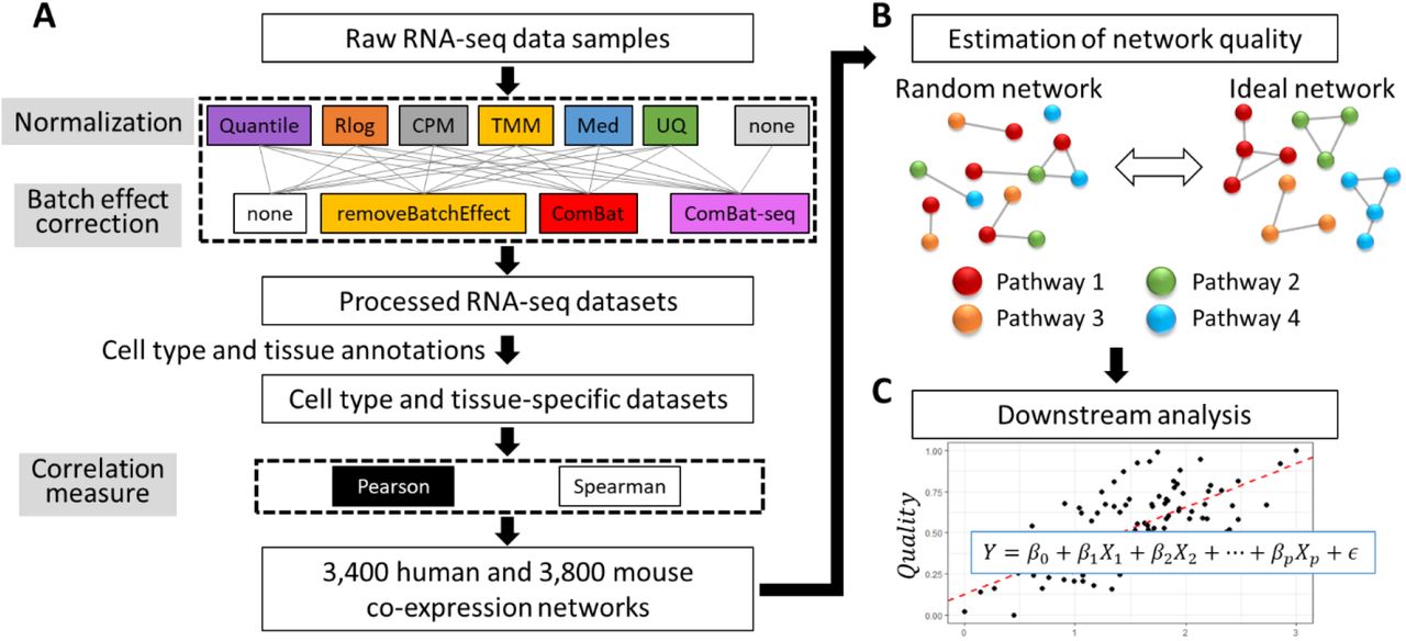
The main goal of this study is to gain insights into which data processing steps are preferable for obtaining high-quality gene co-expression estimates from a large collection of RNA-seq data. To address this issue, we used the RNASeq-er REST API to collect a dataset of 8,796 human and 12,114 mouse bulk RNA-seq samples, from 401 and 630 studies, covering 68 human and 76 mouse cell types and tissues (see Methods; Supplementary Tables S1 and S2) (Petryszak et al., 2017). On these two datasets, we applied combinations of data normalization approaches and batch effect correction approaches (see Figure 1 for a summary of the workflow). As proxies for batches we used the studies that produced each RNA-seq sample (1 study is 1 batch). We also applied the method ComBat-seq on the raw read count data without any prior normalization. The resulting 25 (6 normalizations x 4 batch effect correction approaches, and ComBat-seq without normalization) human and 25 mouse datasets were used to estimate gene co-expression patterns using 2 measures for correlation (Pearson’s correlation and Spearman’s correlation) in the data of each cell type or tissue. This resulted in a total of 7,200 (3,400 human and 3,800 mouse) cell type or tissue-specific gene co-expression networks.

(A) Raw RNA-seq data was processed with 50 different combinations of normalization, batch effect correction, and correlation measures into 7,200 cell type and tissue-specific co-expression networks. (B) Quality of networks was estimated based on the enrichment of functional annotations of correlated genes and regulatory motifs in their promoters. In random networks no common annotations and motifs are expected to be found among correlated genes. In contract, in ideal networks such enrichments should be encountered frequently. Here nodes represent genes and edges co-expression. (C) Quality measures are processed into a single quality score per network, which is used for linear regression analysis.
Defining the quality of co-expression networks
In a next step, we evaluated the quality of each co-expression network. Many studies have used the enrichment of shared functional annotations of correlated genes or regulatory DNA motifs in their promoter sequences as measures of co-expression network quality (Lee et al., 2004; Verleyen et al., 2015; Ballouz et al., 2017; Obayashi et al., 2019). In a high-quality co-expression network, we expect correlated genes to belong to shared pathways or to be controlled by a common regulatory mechanism (Figure 1B). On the other side of the spectrum, in a randomly generated network, any correlation of expression is devoid of biological meaning and there should be no common functions or regulatory mechanisms among correlated genes. In this study, in each network, for every gene, we extracted the set of 100 genes with the highest correlation. We then defined eight quality measures that are based on how frequently we observed enrichment of functional annotations (GO terms) and regulatory motifs (in promoter sequences) among these sets of 100 genes (see Methods for more details). In high-quality networks this frequency should be high, and in low-quality networks it should be low.
We collected the eight quality measures of the 7,200 co-expression networks and applied Principal Component Analysis (PCA). PCA revealed that the eight quality measures were highly consistent and correlated: the first PC explains 81.4% of variability in the quality measures (Supplementary Figure S1A), and had a high correlation with all eight quality measures (range 0.77 to 0.96; Supplementary Figure S1B-C). To facilitate the downstream analysis, we therefore decided to use this first PC as a general quality score (Quality;, see Methods) after rescaling it to the range 0 (worst networks) to 1 (best networks). Figure 2A shows the distribution of Quality; of all networks.
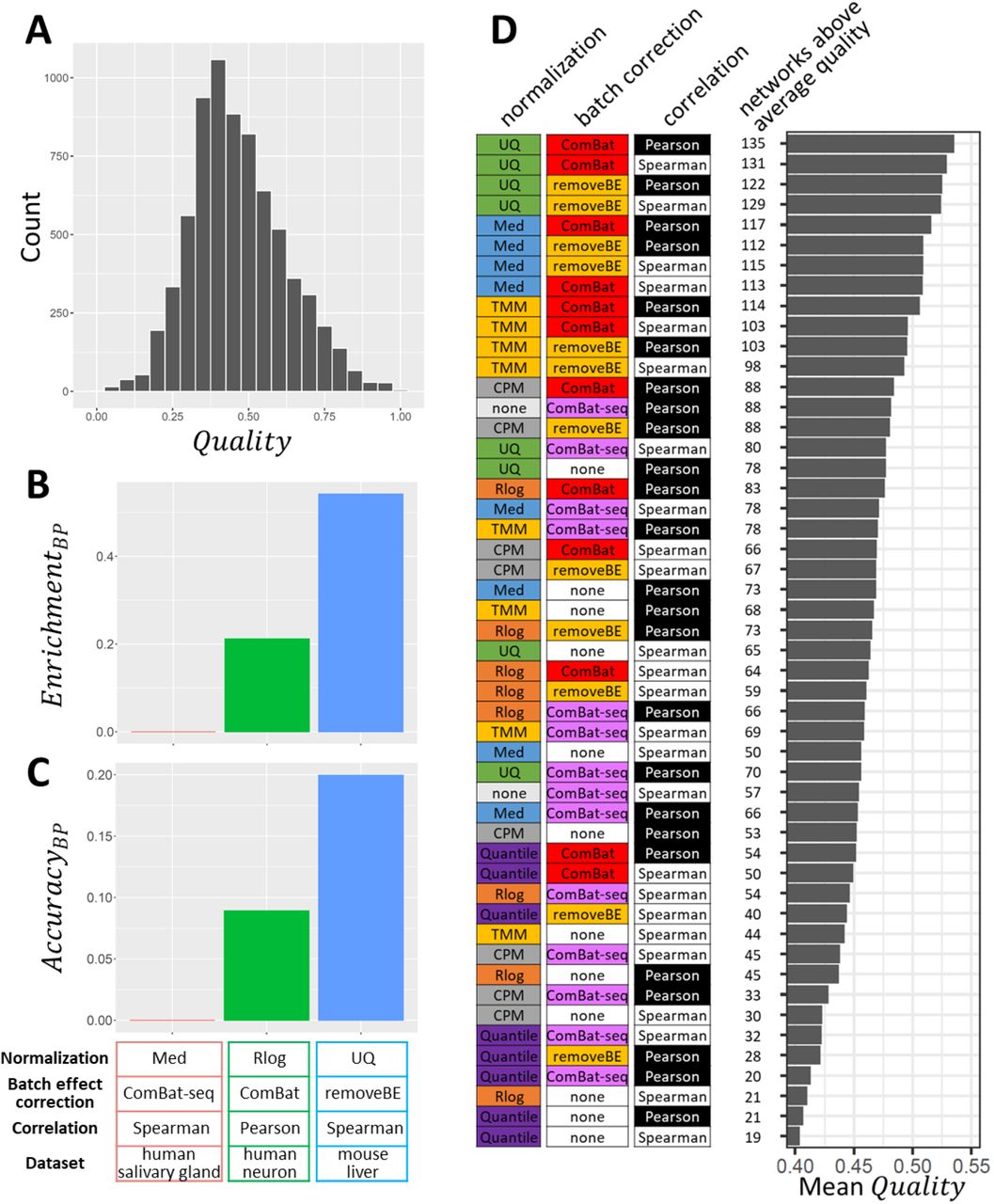
(A) Distribution of the 7,200 general quality scores, Quality; (B-C) Raw quality measures of the worst (red), the median (green), and the best (blue) network for GO Biological Process terms. The frequency of GO term enrichment (B) and their accuracy (C). (D) All 50 evaluated workflows are shown in order of decreasing average quality of the networks they produced. From left to right are shown: the normalization method, batch effect correction method, and measure of correlation used in each workflow. Next, the number of datasets (144 in total) in which the workflow resulted in an above-average quality network is shown, and the mean Quality; of the 144 networks generated using each workflow.
As an illustration, Figure 2B-C show two (of eight) quality measures for the networks with the lowest (Med + ComBat-seq + Spearman applied on human salivary gland data), 50th percentile (Rlog + ComBat + Pearson applied on human neuron data), and highest (UQ + removeBatchEffect + Spearman applied on mouse liver data) Quality;. From the lowest-quality network to the highest-quality network, the measures of quality are progressively increasing. Focusing on the enrichment of Biological Process GO terms (Figure 2B), 0.0% of genes in the lowest-quality network have common annotations among their top 100 correlated genes, while this is 21.2% and 54.2% for the 50th percentile and highest-highest quality network. Enriched Biological Process terms fit with one or more of the known annotations of 0.0%, 8.9%, and 20.0% of the genes in these networks, respectively (Figure 2C). The other six quality measures showed similar trends (Supplementary Figure S2). Together, these results confirm that Quality; reflects the overall quality of the networks accurately.
Figure 2D shows the 50 workflows that we examined, sorted by the average quality of the 144 networks that they each resulted in. The top four workflows all used UQ normalization. Similarly, the top 16 workflows all include a batch processing step, while many of the worst-performing workflows did not treat batch effects. The top-ranking workflow (UQ + ComBat + Pearson) resulted in an above-average network for 135 out of 144 (94%) of the datasets (see also Supplementary Figure S3). This processing workflow therefore appears to be a safe choice.
Modeling the quality of co-expression networks
To gain more quantitative insights into what factors contribute to a high-quality co-expression network and their relative importance, we performed linear regression on the general quality scores Quality; using as predictors: 1) the number of RNA-seq samples on which the network was based (log10 values), 2) the number of batches in the data (log10 values), 3) the species (human or mouse), 4) the data normalization approach, 5) batch correction approach, and 6) the correlation measure. In the next sections, we will first focus on workflows that did not include ComBat-seq. ComBat-seq differs from ComBat and RemoveBatchEffect in that it takes integers as input and therefore cannot be used on data that has already been normalized. Networks generated using ComBat-seq will be treated separately in section “ComBat-seq results in lower-quality networks compared to ComBat and removeBatchEffect”.
The resulting linear model is summarized in Table 1. Despite its simplicity, this model explains 50% of the variability in Quality; (R2 = 0.50). In brief, the model teaches us that a tenfold increase in samples results on average in a 0.27 increase in Quality;. This is consistent with a previous study (Ballouz et al., 2015).
Features (intercept and predictors), estimated coefficients, their standard error, t value and p-value are shown. Qualitative predictors are grouped by species, normalization, batch effect correction and correlation measure.
At the same time, an increase in the number of batches results in a small decrease in Quality;. A number of samples obtained from a small number of studies (=batches) is expected to result in a better network than an equal number of samples generated by many smaller studies.
There was a significant difference between the different normalization methods, with Med and UQ normalization resulting in an average increase of 0.065 and 0.079 in Quality; compared to the baseline (here Quantile normalization, the worse performing method), respectively. These improvements are equivalent to a 74% and 96% increase in sample count, respectively.
Correction of batch effects by removeBatchEffect or by ComBat resulted in better networks. removeBatchEffect increased the Quality; on average by 0.041 and ComBat by 0.048 compared to ignoring batch effects (no correction). These improvements are equivalent to a 41% and 50% increase in sample count, respectively.
Keeping all other things fixed, using Spearman’s correlation instead of Pearson correlation resulted on average in a decrease in the Quality; of about 0.0089 (equivalent to a 7.3% decrease in sample count). Although this is a significant decrease (p = 0.00420), the sample count plays a role in deciding which correlation measure is preferable, and Spearman’s correlation is on average the better approach when the sample count is < 30 (see below).
Note that mouse liver tissue had a high sample count (2,644 samples) compared to other tissues and cell types. As a result, the mouse liver dataset is a high-leverage point for our linear regression analysis. Results presented above are based on a model trained on data that includes the mouse liver data. For completeness, we also present the model trained on data excluding the mouse liver data (Supplementary table S3). In general, similar tendencies were observed.
Below we discuss the roles of sample counts, data normalization, batch effect correction, and correlation measures in more detail.
Importance of sample counts
The best predictor for the quality of the co-expression networks was the number of samples they were based on (Table 1). We observed a clear increase in Quality; as the dataset size increases (Figure 3A). However, it should be noted that this trend follows the law of diminishing returns: if we start at a dataset size of 20, and we increase the number of samples to 100, these additional 80 samples would result in on average an increase in Quality; of 0.19 (the expected increase in quality for a 5-fold higher sample count). However, to further increase the quality by 0.19, we would have to increase the number of samples from 100 to 500, requiring an additional 400 samples. A further increase would require an additional 2,000 samples.

(A) Sample count vs quality of networks. Small points represent the individual networks. Larger points are averages for each dataset. Blue: mouse, red: human datasets. (B) Violin plots of the quality of networks made using each of the six normalization methods. Left: For 59 small datasets (< 50 samples; 354 networks per normalization method). Right: For 26 large datasets (> 200 samples; 156 networks per normalization method).
The collection of hundreds or thousands of additional samples is practically impossible under most circumstances. Therefore, it makes sense to look for data processing steps that can maximize the quality of our networks even in the absence of an increase in samples.
Importance of data normalization approach
Our linear regression analysis revealed clear differences in the average quality of networks generated using the six different normalization methods, with UQ being the best method (Table 1). One weak point of linear regression models is that they assume additivity and independence between predictors. Additional exploratory analysis revealed interactions exist between sample counts and normalization methods: the performance of normalization methods depends on the size of datasets. Figure 3B shows Quality; of networks based on small datasets (< 50 samples; left) and large datasets (> 200 samples; right). While UQ results in high-quality networks in general, the advantage is especially clear on small datasets. In contrast, TMM normalization performed relatively well on large datasets, but less so on small datasets (Figure 3B).
Correcting batch effects in general improves co-expression quality
Our linear regression analysis showed that on average it is better to treat batch effects in gene expression data than to ignore them (Table 1). However, here too, the effect of batch effect correction depends on sample counts, as well as on the number of batches in the dataset (Figure 4). Both removeBatchEffect (Figure 4A) and ComBat (Figure 4B) did not strongly improve networks when the sample count was low (roughly below 50). However, for larger datasets (between 50 and 1,000 samples) both removeBatchEffect and especially ComBat consistently resulted in higher-quality networks (Figure 4A-B). removeBatchEffect on the other hand appeared to have failed to correctly treat batch effects in a few datasets, resulting in worse quality (Figure 4A, indicated datasets). Looking at the quality improvement in function of the number of batches in a dataset (Figure 4D-E), it is clear that batch effect correction offered no clear advantage when a dataset contained few batches (e.g. less than 5). However, for datasets containing 5 or more batches, batch effect correction using ComBat resulted in general in better networks.

(A-C) Difference in quality of co-expression networks based on data with and without treating batch effects in function of sample count, for data treated with removeBatchEffect (A), ComBat (B), and ComBat-seq (C). Positive values indicate an increase in quality in the batch treated networks. (D-F) The same differences in quality in function of the number of batches in each dataset, for removeBatchEffect (D), ComBat (E), and ComBat-seq (F). The average difference in quality is shown in blue for each sample count and for each batch count. A smoothed pattern (generalized additive model) is included in each plot. The plots for ComBat-seq (C,F) compare workflows using ComBat-seq and no normalization step with workflows without batch effect treatment.
In summary, using ComBat to treat batch effects typically led to better co-expression networks, especially for large datasets consisting of data produced in several batches.
Spearman correlation is preferred for small datasets
Linear regression analysis showed that on average there is a small advantage in using Pearson’s correlation over Spearman’s correlation (Table 1). However, here too there the sample count plays an important role: for small datasets (sample count < 30) Spearman’s correlation has an advantage over Pearson’s correlation (Figure 5). For larger datasets Pearson’s correlation leads in general to better co-expression networks, although the difference becomes smaller as the sample count increases.

Difference in the quality (Y axis) of co-expression networks based on Pearson’s correlation and networks based on Spearman’s correlation is shown in function of the number of samples in the datasets (X-axis). Positive values indicate an advantage for Pearson’s correlation, and negative values an advantage for Spearman’s correlation, respectively. The average difference in quality is shown in blue for each dataset. A smoothed pattern (generalized additive model) is included in the plot.
These results make intuitive sense. Pearson’s correlation is more sensitive to extreme values than Spearman’s correlation, which is based on ranks and not on raw values. In small datasets, extreme values have a large leverage on correlation coefficients, adversely affecting networks based on Pearson’s correlation. However, in medium-sized datasets, the influence of extreme values decreases. In those datasets, correlations based on actual values (i.e. Pearson’s correlation) rather than on ranking are better able to capture biological signals.
ComBat-seq results in lower-quality networks compared to ComBat and removeBatchEffect
On average, ComBat-seq did not result in high-quality networks compared to ComBat and removeBatchEffect (Figure 2D). Adding a normalization step following the correction by ComBat-seq did not improve qualities but rather reduced them (Figure 2D). In their study, Zhang and colleagues noted that on some datasets ComBat-seq did not show improved results compared with ComBat (Zhang et al., 2020). In our data, ComBat-seq appeared to lead to lower-quality networks especially in the datasets with more samples (Figure 4C) and those consisting of more batches (Figure 4F). Although the reason for this failure is not clear, we did note that adjustment using ComBat-seq resulted in unrealistically high read counts in a substantial subset of samples. For example, in 821 human samples (out of a total of 8,796) the total read count after correction exceeded 10 billion reads. A subset of genes had extremely high reads counts in some samples. For example, Prh1 had corrected read counts > 1e100 in a subset of human salivary gland samples. These observations suggest that ComBat-seq adjusted a subset of the data to negative binomial distributions that are extremely skewed, negatively affecting the quality of co-expression networks.
The best method depends on the number of samples
Our results suggest that UQ + ComBat + Pearson is in general the preferred approach (Figure 2D and Table 1). However, as discussed above, Spearman correlation offers an advantage on smaller datasets. Figure 6 shows smoothed trends of Quality; in function of sample sizes for all 50 workflows. Five workflows are highlighted: two with the highest average qualities, two with low average qualities, and a default workflow (Rlog + no batch correction + Pearson). Using Spearman correlation clearly leads to better qualities for small datasets, even when using a less well-performing workflow (Quantile + no batch correction + Spearman, Figure 6).

Scatter plot of the number of samples in each dataset (X axis) and Quality; of the networks (Y axis) for all 7,200 networks generated in this study. Smoothed patterns (generalized additive models) are shown for all 50 workflows, with 5 workflows indicated in color.
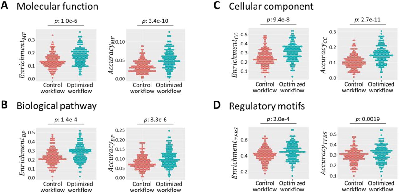
Finally, we returned our focus to the raw quality measures, and compared the networks produced by a default workflow (Rlog + no batch correction + Pearson) with those produced by optimized workflows (UQ + ComBat + Spearman for datasets with < 35 samples, and UQ + ComBat + Pearson otherwise) (Figure 7). For all eight measures, using the optimized approaches resulted in a significant improvement compared to the default workflow (one-sided paired t-tests): the optimized workflows lead to co-expressed genes sharing common functional annotations more frequently (Figure 7A-C left side), as well as shared annotations fitting with the known annotations of genes more frequently (Figure 7A-C right side). The same was true for regulatory motifs in promoter sequences (Figure 7D).

(A-D) (left) Dotplots showing the fraction of genes with enrichment of GO terms and regulatory motifs in networks produced by a default workflow (red) and the optimized workflow (blue). (right) Dotplots showing the fraction of genes with an annotation that fit with enrichment GO terms, and with promoters that contain an instance of an enriched regulatory motif. P values are based on one-sided paired t-tests.
Discussion
We presented a systematic analysis of 50 workflows for generating gene co-expression networks, applied on a large collection of RNA-seq data for 68 human and 76 mouse tissues and cell types. We estimated a general quality score Quality; for the resulting 7,200 networks and used linear regression analysis to gain understanding of the important factors for obtaining a high-quality co-expression network. Here, out aim was to re-analyze existing large RNA-seq expression datasets, that have already been trimmed, aligned to a reference genome, and counted. We focused on the steps of RNA-seq normalization, batch effect correction, and measure of correlation of expression. Other studies have compared between read trimming and alignment approaches in related contexts (Corchete et al., 2020).
We found that co-expression network quality is to a large degree determined by the number of samples on which it is based, as has been reported before (Ballouz et al., 2015). One critical point therefore is to gather as many samples as possible. However, the quality of networks appears to be roughly linearly proportional to the logarithm of the sample count. For every additional increase in quality, an ever-increasing number of additional samples is needed. In practice the number of available samples is always limited, so it makes sense to optimize the data processing workflow to obtain high-quality networks even in the absence of large sample counts.
Treating batch effects in general lead to better networks. On average, ComBat performed better than limma’s removeBatchEffect function. ComBat-seq however performed considerably worse than ComBat and removeBatchEffect. A comparison of batch effect removal approaches for microarray data, found that ComBat outperformed 5 other methods (Chen et al., 2011). Unfortunately, gene co-expression studies still typically ignore batch effects. In our analysis, correcting batch effects using ComBat resulted in improvements to network quality equivalent to a 50% increase in sample count in general. Focusing on larger datasets (>50 samples), the advantage was even more pronounced, equivalent to roughly a doubling in sample count. Clearly, more attention needs to be paid to the issue of batch effects in order to extract the maximum potential out of ever-increasing public gene expression datasets.
We found that some data normalization approaches lead to better networks than others. Especially UQ normalization performed well (Table 1, Figure 2D, and Figure 3B). UQ has also been found to perform relatively well compared with total count normalization (equivalent to CPM normalization in our study) and quantile normalization in the context of predicting differentially expressed genes (Bullard et al., 2010). Other comparisons of RNA-seq normalization methods (outside of the context of co-expression) have come to different and conflicting conclusions (Dillies et al., 2013; Li et al., 2015; Conesa et al., 2016).
The measure of correlation appeared to be less crucial, but Pearson’s correlation seems to have a slight advantage, except when there are only small numbers of samples (<35). In the latter case, Spearman’s correlation seems better.
Although no workflow dominated all others, UQ + ComBat + Pearson (or Spearman for small datasets) resulted in the best network quality overall, and in above-average networks in >90% of the tissues and cell types we examined.
Methods
Gene Expression Data
We used the RNASeq-er REST API of the European Bioinformatics Institute (EBI; https://www.ebi.ac.uk/fg/rnaseq/api/, (Petryszak et al., 2017)) to obtain a list of human and mouse RNA-seq datasets from the European Nucleotide Archive (ENA) with at least 70% of reads mapped to their reference genome.
http://www.ebi.ac.uk/fg/rnaseq/api/tsv/70/getRunsByOrganism/homo_sapiens
http://www.ebi.ac.uk/fg/rnaseq/api/tsv/70/getRunsByOrganism/mus_musculus
Annotation data for each study was downloaded (http://www.ebi.ac.uk/fg/rnaseq/api/tsv/getSampleAttributesPerRunByStudy/<study ID>), and parsed for “cell type” and “organism part” annotation fields. Annotation terms were processed into a list of unique cell types and tissues which were manually checked and turned into a list of consistent terms (removing differences and redundancies in spelling and capitalization). This resulted in consistent cell type or tissue annotations for the RNA-seq samples.
For all samples to which we could assign an annotation, raw read counts per gene were downloaded using the URL:
where <organism> is either “mus_musculus” or “homo_sapiens”. This read count data has been processed using the iRAP pipeline (Fonseca et al., 2014) which includes quality control (including adaptor trimming and filtering out low-quality reads and contaminants), alignment to the reference genome using TopHat2 (Kim et al., 2013), and quantification of the mapped reads per gene using HTSeq (Anders et al., 2015). Because we are focusing here on bulk RNA-seq data we excluded single-cell data from the dataset. This resulted in 9,421 samples for human and 12,787 for mouse. After inspection of the distribution of total number of reads per sample, human samples with less than 2.5 million reads and mouse samples with less than 3 million reads were filtered out. Finally, cell type and tissues with less than 20 samples were removed from the further analysis. The final two datasets contained 8,796 human and 12,114 mouse samples, produced by 401 and 630 studies, covering 68 human and 76 mouse cell types and tissues, respectively (Supplementary Tables S1 and S2).
Gene Expression Data Normalization
On the raw read counts of the two large datasets of human and mouse samples, the following six normalization approaches were used:
Trimmed Mean of M-values (TMM)
One sample is used as reference, and for all other samples, the log ratios for all genes are calculated versus the reference sample (Robinson and Oshlack, 2010). The most highly expressed genes, and the genes with high log ratios are filtered out (hence: “trimmed”). The mean of the remaining log ratios is used as a scaling factor. This normalization methods is the default normalization method of the edgeR function calcNormFactors (McCarthy et al., 2012; Robinson and Oshlack, 2010). In this study, we first removed genes that have less than 1 read per million reads in all samples prior to normalizing the remaining genes.
Counts per million (CPM)
the number of reads per gene is divided by the total number of mapped reads of the sample and multiplied by 1 million ((Dillies et al., 2013), see also (Abbas-Aghababazadeh et al., 2018)).
There are several variations on CPM, describe below, including Upper Quartile and Median.
Upper Quartile (UQ)
counts are divided not by total count but by the upper quartile of non-zero values of the sample (Bullard et al., 2010).
Median (Med)
counts are divided not by total count, but by the median of non-zero values of the sample (Dillies et al., 2013).
Regularized Logarithm (RLog or RLE)
A regularized-logarithm transformation is applied which is similar to a default logarithmic transformation, but in which lower read counts are shrunken towards the genes’ averages across all samples. We applied this normalization using the R package DESeq2 (Love et al., 2014).
Quantile
All samples are normalized to have the same quantiles. We applied this normalization using the function normalizeQuantiles of the limma R package (Ritchie et al., 2015).
Note that methods that correct for differences in gene length (RPKM and FPKM) are not relevant here, since they don’t affect correlation values. Correlation is not changed if one variable is multiplied by a certain factor that is constant over all samples (e.g. 1/gene_length). In this study, these methods would be equivalent to CPM normalization.
We thus obtained 12 normalized datasets (6 each for the human and the mouse data). Each dataset was transformed to log values. To avoid log(0) problems a small pseudo count was added (defined as the 1% percentile of non-zero values in the normalized dataset).
Batch Effect Correction using Combat and limma’s removeBatchEffect Function
On the 12 log-transformed datasets (2 species x 6 normalizations) we applied two batch effect correction methods: ComBat (function ComBat in the sva package) and the removeBatchEffect function of the limma package (Johnson et al., 2007; Ritchie et al., 2015). Both ComBat and removeBatchEffect allow the user to specify the batch covariates to remove from the data (“batch” parameter in both functions). Here, studies were used as substitutes for batches. Users can also give the biological covariates to retain (“mod” parameter in ComBat and “design” parameter in removeBatchEffect). In this study, biological covariates are the cell type or tissue from which the samples were obtained. Both Combat and removeBatchEffect were used using default parameter settings.
In order to be able to treat batch effects in a dataset there can be no confounding between technical and biological covariates. The batch effect removal depends on overlap in biological covariates between batches. Removing batch effects is impossible if all samples of cell type X are present in a batch that contains no samples of cell types that are shared with other batches. In practice, studies often focus on a single cell type, which makes confounding of batches and cell types highly probable. Both the human and mouse datasets could be divided into several subsets with no shared cell types or tissue annotations. Therefore, batch effects were corrected for each of these subsets of samples separately, and finally the treated datasets were merged again into one dataset.
In addition to correcting the data using ComBat and removeBatchEffect we also considered 2 other options. One is to ignore batch effects and use the normalized data directly for estimating gene co-expression. Another is to use ComBat-seq (see next section).
Batch Effect Correction and Normalization using Combat-seq
ComBat-seq differs from ComBat and limma’s removeBatchEffect function in that both its input and output are integer counts, making it more suitable for processing RNA-seq read count data (Zhang et al., 2020). To correct batch effects using ComBat-seq, we therefore gave as input the raw count data (without any normalization step applied to it). In addition, we provided ComBat-seq with the same batch covariates and biological covariates as we used for ComBat and removeBatchEffect. Combat-seq was used with default parameter settings. The output read counts were transformed to log values after adding a pseudocount of 1. These log-transformed data were used for estimating correlation of expression (see next section) without an additional normalization step.
However, quality estimates of the resulting ComBat-seq-processed networks were relatively low compared to those which had been processed using ComBat and removeBatchEffect (Figure 2D and Figure 4C,F), which did include a normalization step. Therefore, to avoid an unfair comparison, we also applied the 6 normalization approaches (TMM, CPM, UQ, Med, Rlog and quantile) on the ComBat-seq output data. Rlog normalization using DEseq2 failed because of the extremely high reads counts in a subset of the data (see also section “ComBat-seq results in lower-quality networks compared to ComBat and removeBatchEffect”). We therefore trimmed all read counts >1e9 to 1e9 before conducting the Rlog normalization.
Together, this resulted in 7 datasets which had been processed using ComBat-seq.
Estimating Correlation of Expression
For each of the 25 data processing combinations (6 normalization methods x 4 batch correction methods, and ComBat-seq without a normalization method), we calculated the correlation of expression between each pair of genes in the log-transformed data for each cell type or tissue. We did this using Pearson’s correlation and Spearman’s rank correlation. Before calculating correlation coefficients in the expression data of a tissue or cell type, genes with general low levels of expression (less than 10 mapped reads in >90% of samples) or with no variation in expression (standard deviation = 0) were removed. The number of samples and number of genes used for calculating co-expression in each tissue and cell type are listed in Supplementary Tables S1 and S2.
Evaluation of Correlation Network Quality
The processing steps described above resulted in 7,200 (3,400 human and 3,800 mouse) cell type or tissue-specific co-expression networks. The main goal of this study is to gain understanding into what are the critical features that distinguish good co-expression networks from bad ones. Because there is no gold standard co-expression network available, we first defined eight measures of quality based on the enrichment of biologically meaningful features (functional annotations of genes and regulatory DNA motifs in promoter sequences) among co-expressed genes. To facilitate comparison between networks, these eight measures were finally combined into a single quality score (see description below).
For each gene X in a co-expression network, we define setX to be the 100 genes with the highest correlation of expression with X (excluding X itself). Our quality measures are based on the enrichment of biologically meaningful features among the genes in setX. These measures should not be interpreted as strict measures of accuracy of for example functional annotation predictions, but rather as rough indicators of quality of the inferred gene co-expression values.
GO enrichment frequency
Genes involved in the same biological process are expected to be co-expressed more frequently than unrelated sets of genes. In a high-quality co-expression network we would expect the genes in setXto share a functional annotation (Figure 1B). In contrast, in a low-quality network (e.g. a randomly generated network) we expect genes in setXto have a random set of annotations. We define EnrichmentMF, EnrichmentBP, and EnrichmentCC as the fraction of genes in a network for which setX contained one or more significantly enriched GO terms (after correction for multiple testing) for Molecular Function (MF), Biological Process (BP) and Cellular Component (CC) GO terms.
GO enrichment accuracy
Where we found setX to have enriched GO terms, we checked if the enriched terms overlapped with the GO terms of gene X. AccuracyMF, AccuracyBP, and AccuracyCC were defined as the fraction of genes in the network for which this was the case for MF, BP, and CC GO terms.
TFBS enrichment frequency
Genes with similar expression profiles are likely to be under the control of a shared regulatory mechanism, including regulation by a similar set of transcription factors (TFs). In a high-quality co-expression network, we would therefore expect the genes in setX to contain a shared set of transcription factor binding sides (TFBSs). We define EnrichmentTNBS as the fraction of genes in a network for which the promoter sequences of setXcontained one or more significantly enriched TFBSs.
TFBS enrichment accuracy
Where we found setX to have enriched TFBSs, we checked if the promoter of gene X contained one or more of those TFBSs. AccuracyTNBS was defined as the fraction of genes in the network for which this was the case.
Correlation between the eight quality measures was high (range 0.60 to 0.98). Principal component analysis (PCA; after standardizing each quality measure to mean 0 and standard deviation 1) revealed that 81.4% of the total variation in the eight quality measures could be explained by the first principal component (PC; Supplementary Figure S1A). We decided to use this first PC as the general quality score, Quality;, after rescaling to the range 0 to 1. The correlation between Quality; and each of the quality measures was high (range 0.77 to 0.96; Supplementary Figure S1B-C). In conclusion, Quality; captures well the general trend of the eight quality measures and simplifies the comparison between the quality of different networks.
Gene Ontology analysis
Gene-to-GO term association data was obtained from the Mouse Genome Informatics website (http://www.informatics.jax.org/) for mouse, and from the EBI database (ftp://ftp.ebi.ac.uk/pub/databases/GO/goa/HUMAN/goa_human.gaf.gz) for human. The basic version of the Gene Ontology (go-basic.obo) was obtained from GO Consortium website (http://geneontology.org/).
GO terms were mapped to their parent terms upward in the GO graph structure. Genes (Entrez IDs) assigned to a particular GO term were also assigned to that term’s parent terms. GO term enrichment in sets of 100 correlated genes (see above) was evaluated using hypergeometric tests: for every GO term the total number of genes associated with the term was compared with the number of genes in the set of 100 genes (Ensembl ids converted to Entrez ids), and a p-value was estimated using a hypergeometric distribution. The Bonferroni correction was used to adjust p-values for multiple testing, and corrected p-values < 0.01 were regarded as significant.
Transcription Factor Binding Site Analysis
Position Weight Matrices (PWMs) were obtained from the JASPAR database (JASPAR_CORE redundant vertebrate PWMs, version of October 2016; 635 PWMs in total) (Mathelier et al., 2016). Promoter sequences (region -500 to +200 around transcription start sites) for all human (hg19/GRCh37) and mouse (mm10/GRCm38) Refseq genes were downloaded using the UCSC Table Browser (Karolchik et al., 2004). We also extracted 10,000 randomly selected regions of the human genome of length 2kb and used them to set a threshold score for each PWM. Threshold scores were set so that each PWM would return on average 1 hit per 5,000 base pairs. A threshold score could be set for 618 PMWs (17 PWMs failed because of low information content).
Vertebrate promoters can be roughly divided into two classes: CpG island-associated promoters and non-CpG island promoters (Lenhard et al., 2012; Illingworth and Bird, 2009). CpG island-associated promoters have on average a higher GC content. To avoid biases caused by differences in GC content and CpG scores, we conducted PWM enrichment analysis as described before (Vandenbon et al., 2016). In brief, we classified all human and all mouse promoter sequences into two classes: promoters with high GC content and high CpG scores, and promoters with low GC content and low CpG scores. For each PWM p, we calculated frp,high, the fraction of high GC content promoters that contain a hit for p. Similarly, we calculated frp,low, the fraction of low GC content promoters that contain a hit for p. For the prediction of enriched PWM motifs in a set of promoters D, we counted hp,D, the number of sequences that contain a hit for p, as well as the number of sequences in D that were classified in the high GC content class (nhigh) and in the low GC content class (nlow), respectively. Finally, using a binomial distribution, we calculated the probability of observing hp,D or more hits for p in a set of nhigh high GC content and nlow low GC content sequences, given frp,high and frp,low. This probability was corrected for multiple testing using the Bonferroni correction, and PWMs with a corrected p value < 0.01 were considered as significantly enriched in the input set D.
Linear regression analysis
We conducted least squares regression using the lm() function in R. As response variable we used Quality;, and as predictors we used 1) the number of RNA-seq samples on which the network was based (log10 values), 2) the number of batches in the data (log10 values), 3) the species (human or mouse), 4) the data normalization approach, 5) batch correction approach, and 6) the correlation measure. For the categorical predictors (i.e. species, data normalization approach, batch correction approach and correlation measure) lm()uses dummy variables with values 0 and 1. The baseline levels of these categorical variable were set in a way that facilitates interpretation of the results (Table 1).
Data Availability
Both the human and the mouse RNA-seq datasets are available in figshare with DOIs doi.org/10.6084/m9.figshare.14178446.v1 and doi.org/10.6084/m9.figshare.14178425.v1. These datasets include 1) the raw read counts of genes in all RNA-seq samples, 2) the same RNA-seq data after UQ normalization and batch effect removal using ComBat, which is in general the best processing workflow according to our study, 3) annotation data assigning a study ID and cell type or tissue to each RNA-seq sample, and 4) A list of each cell type or tissue included in the dataset along with its sample count.
End Notes
Author Contributions
A.V. conceived of the project and methodology, ran the analyses, and wrote the manuscript.
Conflict of Interest
The authors declare that they have no competing interests.
Acknowledgements
We thank Prof. Yoshio Koyanagi and the members of the Lab. of Systems Virology (Kyoto University), Prof. Kenta Nakai and the member of the Lab. of Functional Analysis in silico (Tokyo University), Prof. Wataru Fujibuchi (Kyoto University), and Dr. Diego Diez (Osaka University) for helpful discussions and advice. This work was supported by a KAKENHI Grant-in-Aid for Scientific Research (C) (20K06609) by the Japan Society for the Promotion of Science (JSPS).
Footnotes
Contact: alexisvdb{at}infront.kyoto-u.ac.jp
References


