

Abstract
Biological networks constructed from varied data, including protein-protein interactions, gene expression data, and genetic interactions can be used to map cellular function, but each data type has individual limitations such as bias and incompleteness. Unsupervised network integration promises to address these limitations by combining and automatically weighting input information to obtain a more accurate and comprehensive result. However, existing unsupervised network integration methods fail to adequately scale to the number of nodes and networks present in genome-scale data and do not handle partial network overlap. To address these issues, we developed an unsupervised deep learning-based network integration algorithm that incorporates recent advances in reasoning over unstructured data – namely the graph convolutional network (GCN) – and can effectively learn dependencies between any input network, such as those composed of protein-protein interactions, gene co-expression, or genetic interactions. Our method, BIONIC (Biological Network Integration using Convolutions), learns features which contain substantially more functional information compared to existing approaches, linking genes that share diverse functional relationships, including co-complex and shared bioprocess annotation. BIONIC is scalable in both size and quantity of the input networks, making it feasible to integrate numerous networks on the scale of the human genome.
Introduction
High-throughput genomics projects produce massive amounts of biological data for thousands of genes. The results of these experiments can be represented as functional gene-gene interaction networks, which link genes or proteins of similar function1. For example, protein-protein interactions describe transient or stable physical binding events between proteins2–7. Gene co-expression profiles identify genes that share similar patterns of gene expression across multiple experimental conditions, revealing co-regulatory relationships between genes8,9. Genetic interactions (e.g. synthetic lethal) link genes that share an unexpected phenotype when perturbed simultaneously, capturing functional dependencies between genes10,11. Each of these data typically measures a specific aspect of gene function and have varying rates of false-positives and negatives. Data integration has the potential to generate more accurate and more complete functional networks. However, the diversity of experimental methods and results makes unifying and collectively interpreting this information a major challenge.
Numerous methods for network integration have been developed with a range of benefits and disadvantages. For example, many integration algorithms produce networks that retain only global topological features of the original networks, at the expense of important local relationships12–15, while others fail to effectively integrate networks with partially disjoint node sets16,17. Some methods encode too much noise in their output, for instance by using more dimensions than necessary to represent their output, thereby reducing downstream gene function and functional interaction prediction quality12–16. Most of these approaches do not scale in the number of networks or in the size of the networks to real world settings14,16,18. Supervised methods have traditionally been the most common network integration approach15,18–20. These methods, while highly successful, require labelled training data to optimize their predictions of known gene functions, and thus risk being biased by and limited to working with known functional descriptions.
Unsupervised methods have more recently been explored to address this potential weakness. They automatically identify network structure, such as modules, shared across independent input data and can function in an unbiased manner, using techniques such as matrix factorization12–14, cross-diffusion16, low-dimensional diffusion state approximation17 and multimodal autoencoding21. Theoretically, unsupervised network integration methods can provide a number of desirable features such as automatically retaining high-quality gene relationships and removing spurious ones, inferring new relationships based on the shared topological features of many networks in aggregate, and outputting comprehensive results that cover the entire space of information associated with the input data, all while remaining agnostic to any particular view of biological function.
Recently, new methods have been developed that focus on learning compact features over networks22,23. These strategies aim to capture the global topological roles of nodes (i.e. genes or proteins) and reduce false positive relationships by compressing network-based node features to retain only the most salient information. However, this approach produces general purpose node features that cannot be tuned to capture the unique topology of any particular input network, which may vary greatly with respect to other input networks. Recent advances in deep learning have addressed this shortcoming with the development of the graph convolutional network (GCN), a general class of neural network architectures which are capable of learning features over networks24–27. GCNs can learn compact, denoised node features that are trainable in a network-specific fashion. Additionally, the modular nature of the GCN enables the easy addition of specialized neural network architectures to accomplish a task of interest, such as network integration, while remaining scalable to large input data. Compared to general-purpose node feature learning approaches22,23, GCNs have demonstrated substantially improved performance for a range of general network tasks, a direct result of their superior feature learning capabilities24,27. These promising developments motivate the use of the GCN for gene and protein feature learning on real-world, biological networks, which are large and numerous, and feature widely variable network topologies.
Here we present a general, scalable deep learning framework for network integration called BIONIC (Biological Network Integration using Convolutions) which uses GCNs to learn holistic gene features given many different input networks. To demonstrate the utility of BIONIC, we integrate three diverse, high-quality gene or protein interaction networks to obtain integrated gene features that we compare to a range of function prediction benchmarks. We compare our findings to those obtained from a wide range of integration methodologies12,17, and we show that BIONIC features perform well at both capturing functional information, and scaling in the number of networks and network size, while maintaining gene feature quality.
Results
Method overview
BIONIC uses the GCN neural network architecture to learn optimal gene (protein) interaction network features individually, and combines these features into a single, unified representation for each gene (Fig. 1). First, the input data, if not already in a network format, are converted to networks (e.g. by gene expression profile correlation). Each input network is then run through an independent GCN to produce network-specific gene features. Using an independent GCN for each network enables BIONIC to learn the parameters that capture unique input network features. Each input network is passed through its corresponding GCN multiple times (two times in our experiments - see Methods) to capture higher-order gene neighborhood information24 and, with the addition of residual connections, BIONIC produces both local and global gene features28. The network-specific features are then summed through a stochastic gene dropout procedure to produce unified gene features which can be used in downstream tasks, such as functional module detection or gene function prediction. To optimize the functional information encoded in its integrated features, BIONIC must have a relevant training objective that facilitates capturing salient features across multiple networks. Here, BIONIC uses an autoencoder design and reconstructs each input network by mapping the integrated features to a network representation (decoding) and minimizing the difference between this reconstruction and the original input networks. By optimizing the fidelity of the network reconstruction, BIONIC forces the learned gene features to encode as much salient topological information present in the input networks as possible and reduces the amount of spurious information encoded. Indeed, in many cases, inputting even individual networks into BIONIC improves their performance on several benchmarks (below) compared to their original raw format (Fig. S1).
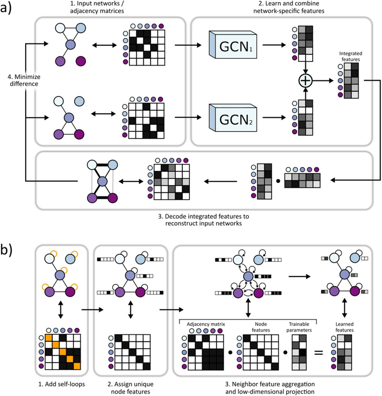
a) 1. Gene interaction networks input into BIONIC are represented as adjacency matrices. 2. Each network is passed through a graph convolution network (GCN) to produce network-specific gene features which are then combined into an integrated feature set which can be used for downstream tasks such as functional module detection. 3. BIONIC attempts to reconstruct the input networks by decoding the integrated features through a dot product operation. 4. BIONIC trains by updating its weights to reproduce the input networks as accurately as possible. b) The GCN architecture functions by 1. adding self-loops to each network node, 2. assigning a “one-hot” feature vector to each node in order for the GCN to uniquely identify nodes and 3. propagating node features along edges followed by a low-dimensional, learned projection to obtain updated node features which encode network topology.
Few biological networks are comprehensive in terms of genome coverage and the overlap in the set of genes captured by different networks is often limited. Some methods ignore this problem by simply integrating genes that are common to all networks16, resulting in progressively smaller gene sets as more networks are added, whereas others unintentionally produce gene features that are dependent on whether a gene is present in all or only some of the input networks17. Integration methods generally require each input network to have the same set of genes, so to produce an integrated result that encompasses genes present across all networks (i.e. the union of genes) each network must be extended with any missing genes12,15–17,21. However, existing methods do not distinguish between genes that have zero interactions due to this extension or genes with zero measured interactions in the original data12,15–17. To address this, BIONIC implements a masking procedure which prevents penalizing the reconstruction fidelity of gene interaction profiles in networks where the genes were not originally present (see Methods).
Evaluation criteria
We compared the quality of BIONIC’s learned features to two established unsupervised integration methods, a matrix factorization method12 and a diffusion state approximation method17, as well as a naive union of networks as a baseline. We assessed the quality of these method outputs using three evaluation criteria: gene co-annotation precision-recall, gene module detection, and supervised gene function prediction. First, we used an established precision-recall evaluation strategy11,29 to compare pairwise gene-gene relationships produced by the given method to sets of known positive and negative relationships (co-annotations). Second, we evaluated the capacity of each method to produce biological modules by comparing clusters computed from the output of each method to known modules such as protein complexes, pathways, and biological processes. Finally, the supervised gene function prediction evaluation determines how discriminative the method outputs are for predicting known gene functions. Here, a portion of the genes were held out and used to evaluate the accuracy of a support vector machine classifier30 trained on the remaining gene features to predict known functional classes17.
BIONIC produces high quality gene features
We first used BIONIC to integrate three high-quality yeast networks: a comprehensive network of correlated genetic interaction profiles (4,529 genes, 33,056 interactions)11, a co-expression network derived from transcript profiles of yeast strains carrying deletions of transcription factors (1,101 genes, 14,826 interactions)9, and a protein-protein interaction network obtained from an affinity-purification mass-spectrometry assay (2,674 genes, 7,075 interactions)5, which combine for a total of 5,232 unique genes and 53,351 unique interactions (Fig. 2, Supplementary Data File 1).

a) Co-annotation prediction, module detection, and gene function prediction evaluations for three yeast networks integrated by the tested unsupervised network integration methods. The co-annotation and module detection standards contain between 1786 and 4170 genes overlapping the integration results. The module detection standards define between 107 and 1803 modules. The IntAct, KEGG and GO BP gene function prediction standards cover 567, 1770 and 1211 genes overlapping the integration results, and 48, 53 and 63 functional classes, respectively (see Supplementary Data File 2). Error bars indicate the 95% confidence interval. b) Evaluation of integrated features using high-level functional categories, split by category. Each category contains between 21 and 149 genes overlapping the integration results (denoted by counts above the heatmap columns, see Supplementary Data File 2) c) Top row: Comparison of overlap scores between known complexes and predicted modules, between BIONIC and the input networks. Each point is a protein complex. The x and y axes indicate the overlap (Jaccard) score, where a value of 0 indicates no members of the complex were captured, and 1 indicates the complex was captured perfectly. The diagonal indicates complexes where BIONIC and the given input network have the same score. Points above the diagonal are complexes where BIONIC outperforms the given network, and points below the diagonal are complexes where BIONIC underperforms the network. The arrows indicate the SEC62-SEC63 complex, shown in d). A Venn diagram describes the overlap of captured complexes (defined as a complex with an overlap score of 0.5 or higher) between the input networks and BIONIC integration. Bottom row: The distribution of overlap scores between predicted and known complexes for each network and BIONIC. The dashed line indicates the distribution mean. d) Functional relationships between predicted SEC62-SEC63 complex members and genes in the local neighborhood, as given by the three input networks and corresponding BIONIC integration of these networks. The predicted cluster best matching the SEC62-SEC63 complex in each network, based on the module detection analysis in a), is circled. The overlap score of the predicted module with the SEC62-SEC63 complex is shown. Edges correspond to protein-protein interactions in PPI5, Pearson correlation between gene profiles in Co-expression9 and Genetic Interaction11 networks, and cosine similarity between gene features in the BIONIC integration. Edge weight corresponds to the strength of the functional relationship (correlation), where a heavier edge implies a stronger functional connection. PPI = Protein-protein interaction, GO = Gene Ontology, BP = Biological process.
We compared BIONIC integrated features to a naive union of networks integration approach (Union), a non-negative matrix tri-factorization approach (iCell)12, and a low-dimensional diffusion state approximation approach (Mashup)17. These unsupervised integration methods cover a diverse set of methodologies and the major possible output types (networks for Union and iCell, features for Mashup). Compared to these approaches, BIONIC integrated features have superior performance on all evaluation criteria over three different functional benchmarks: IntAct protein complexes31, Kyoto Encyclopedia of Genes and Genomes (KEGG) pathways32 and Gene Ontology biological processes (GO)33 (Fig. 2a, Supplementary Data File 2). As an additional test, BIONIC produces high-quality features that accurately predict a diverse set of yeast biological process annotations per gene11 (Fig. 2b). Some categories in this latter test do better than others. These performance patterns were mirrored in the individual input networks (Fig. S2), indicating that this is the result of data quality, rather than method bias. Thus, BIONIC can capture high-quality functional information across diverse input networks, network topologies and gene function categories, and its features can be used to accurately identify pairwise gene co-annotation relationships, functional modules, and predict gene function.
Applying our benchmark-optimized module detection analysis to the individual input networks, we observed that features obtained through BIONIC network integration often outperformed the individual input networks at capturing functional modules (Fig. S1) and captured more modules (Fig. 2c, Supplementary Data File 3), demonstrating the utility of the combined features over individual networks for downstream applications such as module detection. Here we treated the network adjacency profiles (rows in the adjacency matrix) as gene features. We then examined how effectively the input networks and integrated BIONIC features captured known protein complexes, by matching each individual known complex to its best matching predicted module and quantifying the overlap (Fig. 2c). We then compared the overlap scores from each network to the BIONIC overlap scores to identify complexes where BIONIC performs either better or worse than the input networks. Of 330 protein complexes tested, BIONIC strictly improved 204, 292, 171 complex predictions and strictly worsened 103, 27, 128 complex predictions compared to the input protein-protein interaction, co-expression, and genetic interaction networks, respectively. The distributions of complex overlap scores for each dataset indicate that BIONIC predicts protein complexes more accurately than the input networks on average. Indeed, if we use an overlap score of 0.5 or greater to indicate a successfully captured complex, BIONIC captures 96 complexes, compared to 81, 3 and 72 complexes for the protein-protein interaction, co-expression, and genetic interaction networks, respectively (Fig. 2c). We also repeated this module analysis, instead optimizing the clustering parameters on a per-module basis, an approach that tests how well each network and BIONIC perform at capturing modules under optimal clustering conditions for each module. Here too, BIONIC captured more modules and with a greater average overlap score than the input networks (Fig. S3, S4, Supplementary Data File 4).
To understand how BIONIC is able to improve functional gene module detection compared to the input networks, we examined the SEC62-SEC63 complex, which was identified in our benchmark-optimized module evaluation (Fig. 2a) as an example to show how BIONIC effectively combines gene-gene relationships across different networks and recapitulates known biology. The SEC62-SEC63 complex is an essential protein complex required for post-translational protein targeting to the endoplasmic reticulum and is made up of the protein products of four genes - SEC62, SEC63, SEC66, and SEC7234. We found that the cluster which best matched the SEC62-SEC63 complex in each input network only captured a subset of the full complex, or captured many additional members not known to be SEC62-SEC63 members (Supplementary Data File 3). The BIONIC module, however, contained the four known subunits of the SEC62-SEC63 complex, along with one member of the translocation complex, which shares a closely related function to the SEC62-SEC63 complex. We examined the best-matching clusters and their local neighborhood, consisting of genes that show a direct interaction with predicted members of the SEC62-SEC63 complex, in the input networks, and in a profile similarity network obtained from the integrated BIONIC features of these networks (Fig. 2d). We found that the PPI network captured two members of the SEC62-SEC63 complex, with an additional member in the local neighborhood. Interactions between members of the complex are sparse however, preventing the clustering algorithm from identifying the full complex. The co-expression network only identified one complex member, and the local neighborhood of the best matching module does not contain any additional known complex members. The genetic interaction network is able to connect and localize all members of the SEC62-SEC63 complex, though the presence of three additional predicted complex members obscures the true complex. Finally, BIONIC utilizes the interaction information present in the PPI and genetic interaction networks to fully identify the SEC62-SEC63 module, with only one additional predicted complex member. This analysis demonstrates the utility of BIONIC for identifying meaningful biological modules in sparse networks and noisy networks by clustering its learned features. Indeed, when we optimized the module detection procedure to specifically resolve the SEC62-SEC63 complex, we found that BIONIC was able to capture the complex with a higher overlap score than any of the input networks and other integration methods (Supplementary Data File 4).
BIONIC is scalable in number of networks and number of genes
High-throughput experiments have led to a rapidly growing wealth of biological networks. For the major studied organisms, including yeast and human, there are hundreds of available networks which, when unified, often include close to a genome-wide set of genes. Ideally, all of these networks could be unified to improve available gene function descriptions. However, many unsupervised integration methods either cannot run with many input networks or networks with large numbers of genes, or they scale with reduced performance. To test network input scalability, we randomly sampled progressively larger sets of yeast gene co-expression networks (Fig. 3a, Supplementary Data File 1) and assessed the performance of the resulting integrations of these sets. We similarly tested node scalability by randomly subsampling progressively larger gene sets of four human protein-protein interaction networks3,6,7,35 (Fig. 3b, Supplementary Data File 1). BIONIC can integrate numerous networks (Fig. 3a), as well as networks with many nodes (Fig. 3b), outperforming all other methods assessed for progressively more and larger networks. To achieve this scalability, BIONIC takes advantage of the versatile nature of deep learning technology by learning features for small batches of genes and networks at a time, reducing the computational resources required for any specific training step. To learn gene features over large networks, BIONIC learns features for random subsets of genes at each training step, and randomly subsamples the local neighborhoods of these genes to perform the graph convolution (see Methods), maintaining a small overall computational footprint. This subsampling allows BIONIC to integrate networks with many genes, whereas methods like Mashup can only do so with an approximate algorithm which substantially reduces performance (Fig. S5). To integrate many networks, BIONIC uses a network-wise sampling approach, where a random subset of networks is integrated at a time during each training step. This reduces the number of parameter updates required at once, since only GCNs corresponding to the subsampled networks are updated in a given training step.

a) Performance of integrating various numbers of randomly sampled yeast co-expression input networks on KEGG Pathways gene co-annotations. b) Performance of integrating four human protein-protein interaction networks over a range of sub-sampled nodes (genes) on CORUM Complexes protein co-annotations. In these experiments the Mashup method failed to scale to a) 15 or more networks and b) 4000 or more nodes, as indicated by the absence of bars in those cases (see Methods). Error bars indicate the 95% confidence interval.
Discussion
We present BIONIC, a new deep-learning algorithm that extends the graph convolutional network architecture to integrate biological networks. We demonstrated that BIONIC produces gene features which capture functional information well when compared to other unsupervised methods12,17 as determined by a range of benchmarks and evaluation criteria, covering a diverse set of downstream applications such as gene co-annotation prediction, functional module detection and gene function prediction. We have also shown that BIONIC performs well for a range of numbers of input networks and network sizes, where established methods are not able to scale past relatively few networks or scale only with reduced performance.
In a global sense, BIONIC performs well and captures relevant functional information across input networks. However, input networks do not have uniform quality and some networks may only describe certain types of functional relationships effectively (such as those within a particular biological process) while obscuring other relationships. Indeed, while BIONIC is able to capture a greater number of functional modules than a given input network alone (Fig. 2c, Fig. S3), BIONIC does not capture every functional module present in the input networks (Fig. 2c, Fig. S4, Supplementary Data Files 3, 4). This is likely due to some networks obscuring signals present in other networks. Implementing more advanced input network feature weighting or learning these weightings should ensure that high-quality information is preferentially encoded in the learned features and that low-quality information is not enriched. This may additionally help to identify which functional relationships are driven by which networks and network types - indicating which parts of the functional spectrum have good or poor coverage and identifying areas to target for future experimental work.
Interestingly, the naive union of networks approach performs surprisingly well, motivating its inclusion as a baseline in our network integration algorithm assessments. While the union network contains all possible relationships across networks, it likely contains relatively more false-positive relationships in the integrated result, since all false-positives in the input networks are retained by the union operation.
Finally, BIONIC learns gene features based solely on their topological role in the given networks. GCN’s are able to incorporate a priori node features. A powerful future addition to BIONIC would be to include gene or protein features such as amino acid sequence36, protein localization37, morphological defect38, or other non-network features to provide additional context for genes in addition to their topological role. Continued development of integrative gene function prediction using deep learning-based GCN and encoder-decoder technologies will enable us to map gene function more richly and at larger scales than previously possible.
Author Contributions
DTF developed the method, performed the experiments. DTF, CB, GDB and BW wrote the manuscript. CB, GDB and BW conceived of and supervised the project.
Competing Interests
The authors declare no competing interests.
Online Methods
Network Preprocessing
The yeast protein-protein interaction network5 and human protein-protein interaction networks3,6,7,35 were obtained from BioGRID39, genetic interaction profiles11 were obtained directly from the published supplementary data of Costanzo et al. 2016, and gene expression profiles were obtained from the SPELL database8. To create a network from the genetic interaction profiles, genes with multiple alleles were collapsed into a single profile by taking the maximum profile values across allele profiles. Pairwise Pearson correlation between the profiles was then calculated, and gene pairs with a correlation magnitude greater than or equal to 0.2 were retained as edges, as established11. For the gene expression profiles, networks were constructed by retaining gene pairs with a profile Pearson correlation magnitude in the 99.5th percentile. Co-expression and genetic interaction networks had their edge weights normalized to the range [0, 1].
Obtaining Integrated Results
The naive union of networks benchmark was created by taking the union of node sets and edge sets across input networks. For edges common to more than one network, the maximum weight was used. iCell results were obtained by running the algorithm with default parameters. Mashup and BIONIC were set to have the same dimensionality (512 for all experiments). All other Mashup parameters were defaults. For human networks, an SVD approximation feature of BIONIC was used (see Implementation Details below) to compute low-dimensional initial node features and preserve memory. BIONIC features used in this study are found in Supplementary Data File 5.
Benchmark Construction
Functional benchmarks were derived from GO Biological Process ontology annotations, KEGG pathways and IntAct complexes for yeast, and CORUM complexes for human (Supplementary Data File 2). Analyses were performed using positive and negative gene pairs, clusters or functional labels obtained from the standards as follows: the GO Biological Process benchmark was produced by filtering IEA annotations, as they are known to be lower quality, removing genes with dubious open reading frames, and filtering terms with more than 30 annotations (to prevent large terms, such as those related to ribosome biogenesis, from dominating the analysis40). For the co-annotation benchmark, all gene pairs sharing at least one annotation were retained as positive pairs, while all gene pairs not sharing an annotation were considered to be negative pairs. KEGG, IntAct and CORUM benchmarks were produced analogously, without filtering.
For the module detection benchmark, clusters were defined as the set of genes annotated to a particular term, for each standard. Modules of size 1 (singletons) were removed from the resulting module sets as they are uninformative.
The supervised standards were obtained by treating each gene annotation as a class label, leading to genes with multiple functional classes (i.e. a multilabel classification problem). The standards were filtered to only include classes with 20 or more members for GO Biological Process and KEGG, or 10 members for IntAct. This was done to remove classes with very few data points, ensuring more robust evaluations.
The granular function standard in Fig. 2b was obtained from the Costanzo et al. 2016 supplementary materials. Any functional category with fewer than 20 gene members was removed from the analysis to ensure only categories with robust evaluations were reported.
Evaluation Methods
We used a precision-recall (PR) based co-annotation framework to evaluate individual networks and integrated results. We used PR instead of receiving operator curve (ROC) because of the substantial imbalance of positives and negatives in the pairwise benchmarks for which ROC would overestimate performance. Here, we computed the pairwise cosine similarities between gene profiles in each network or integration result. Due to the high-dimensionality of the datasets, cosine similarity is a more appropriate measure than Euclidean distance since the contrast between data points is reduced in high-dimensional spaces under Euclidean distance41. PR operator points were computed by varying a similarity threshold, above which gene or protein pairs are considered positives and below which pairs are considered negative. Each set of positive and negative pairs was compared to the given benchmark to compute precision and recall values. To summarize the PR curve into a single metric, we computed average precision (AP) given by:
 where n is the number of operator points (i.e. similarity thresholds) and Pi and Ri are the precision and recall values at operator point i respectively. This gives the average of precision values weighted by their corresponding improvements in recall. We chose this measure over the closely related area under the PR curve (AUPRC) measure since AUPRC interpolates between operator points and tends to overestimate actual performance42.
The module detection evaluation was performed by clustering the integrated results from each method and comparing the coherency of resulting clusters with the module-based benchmarks. Since the benchmarks contain overlapping modules (i.e. one gene can be present in more than one module) which prevents the use of many common clustering evaluation metrics (since these metrics assume unique assignment of gene to cluster), the module sets are subsampled during the evaluation to ensure there are no overlapping modules (the original module sets are used as-is for the per-module-optimized experiments in Fig. S4, Supplementary Data File 3). Next, the integrated results are hierarchically clustered with a range of distance metrics (Euclidean and cosine), linkage methods (single, average and complete) and thresholds to optimize benchmark comparisons over these clustering parameters (this is done for all methods that are compared). The resulting benchmark-optimized cluster sets are compared to the benchmark module sets by computing adjusted mutual information (AMI) - an information theoretic comparison measure which is adjusted to normalize against the expected score from random clustering. The highest AMI score for each integration approach is reported - ensuring the optimal cluster set for each dataset across clustering parameters is used for the comparison and that our results are not dependent on clustering parameters. Finally, this procedure is repeated ten times to control for differences in scores due to the cluster sampling procedure. The sets of clustering parameter-optimized BIONIC clusters obtained from the Fig. 2 integration for each standard are in Supplementary Data File 3.
To perform the supervised gene function prediction evaluation, ten trials of five-fold cross validation were performed using support vector machine (SVM) classifiers each using a radial basis function kernel30. The classifiers were trained on a set of gene features obtained from the given integration method with corresponding labels given by the IntAct, KEGG and GO Biological Process supervised benchmarks in a one-versus-all fashion (since each individual gene has multiple labels). Each classifier’s regularization and gamma parameters were tuned in the validation step. For each trial, the classifier results were evaluated on a randomized held out set consisting of 10% of the gene features not seen during training or validation and the resulting classification accuracy was reported.
The granular functional evaluation in Fig. 2b was generated by computing the average precision (as mentioned in the precision-recall evaluation framework description) for the gene subsets annotated to the given functional categories.
To perform the module comparison analysis in Fig. 2c, we additionally applied the module detection analysis performed in Fig. 2a to the input networks. Here, the interaction profiles of the networks were treated as gene features and the clustering parameters were optimized to best match the IntAct complexes standard. We compared the resulting module sets from the input networks and BIONIC features to known protein complexes given by the IntAct standard. For each complex in the standard, we reported the best matching predicted module in each dataset as determined by the overlap (Jaccard) score between the module and the known complex (Supplementary Data File 3). To generate the Venn diagram, we defined a complex to have been captured in the dataset if it had an overlap score of 0.5 or greater with a predicted module.
To perform the SEC62-SEC63 module analysis in Fig. 2d, we analyzed the predicted module in each dataset that had the highest overlap score with the SEC62-SEC63 complex. We created a network from the BIONIC features by computing the cosine similarity between all pairs of genes and setting all similarities below 0.5 to zero. The resulting non-zero values were then treated as weighted edges to form a network. We extracted a subnetwork from each of the protein-protein interaction, co-expression, genetic interaction and newly created BIONIC networks, consisting of the best scoring predicted module and the genes showing direct interactions with those in the predicted module. We laid out these networks using the prefuse force-directed algorithm in Cytoscape43. The edges in the protein-protein interaction network correspond to direct, physical interactions, and the edges in the co-expression and genetic interaction networks correspond to the pairwise Pearson correlation of the gene profiles, as described above.
Network Scaling Experiment
To perform the network scaling experiment, we sampled subsets of the yeast co-expression networks (Supplementary Data File 1). We performed 10 integration trials for each network quantity, and these trials were paired (i.e. each method integrated the same randomly sampled sets of networks). The average precision scores of the resulting integrations with respect to the KEGG pathways co-annotation standard (Supplementary Data Files 2) were then reported. The Mashup method did not scale to the 15 network input size or beyond on a machine with 64GB of RAM.
Node Scaling Experiment
The node scaling experiment was performed by subsampling the nodes of four large human protein-protein interaction networks3,6,7,35 (Supplementary Data File 1) for a range of node quantities and integrating these subsampled networks. Ten trials of subsampling were performed for each number of nodes (paired, as above) and the average precision scores with respect to the CORUM complexes co-annotation standard (Supplementary Data File 2) were reported. The Mashup method did not scale to 4000 nodes or beyond on a machine with 64GB of RAM.
BIONIC Method Overview
An undirected input network can be represented by its adjacency matrix A where Ai j = Aji > 0 if node i and node j share an edge and Aij = Aji = 0 otherwise. BIONIC first preprocesses each input network to contain the union of nodes across all input networks and ensures the corresponding row and column orderings are the same. In instances where networks are extended to include additional nodes not originally present in them (so all input networks share the same union set of nodes), the rows and columns corresponding to these nodes are set to 0.
BIONIC encodes each input network using instances of a GCN variant known as the Graph Attention Network (GAT)27. The GAT has the ability to learn alternative network edge weights, allowing it to downweight or upweight edges based on their importance for the network reconstruction task. In the original formulation, the GAT assumes binary network inputs. We modify the GAT to consider a priori network edge weights. The GAT formulation is then given by:
 where
where

Here, W is a trainable weight matrix which projects aggregated node features into another feature space, a is a vector of trainable attention coefficients which determine the resulting edge weighting, hi is the feature vector for node i (that is, the ith row of feature matrix H), ∥ denotes the concatenation operation and a corresponds to a nonlinear function (in our case a leaky rectified linear unit (LeakyReLU)) which produces more sophisticated features than linear maps. (2) corresponds to a node neighborhood aggregation and projection step which incorporates an edge weighting scheme (3). In practice, several edge weighting schemes (known as attention heads) are learned and combined simultaneously, resulting in:
 where k is the number of attention heads. This is done to stabilize the attention learning process, as per the author’s original results27. In our experiments we use 10 attention heads per GAT encoder, each with a hidden dimension of 64.
Initial node features Hinit are a one-hot encoding so that each node is uniquely identified (i.e. Hinit = I where I is the identity matrix). These features are first mapped to a lower dimensional space through a learned linear transformation to reduce memory footprint and improve training time. Due to the current technical limitations in how the underlying deep learning framework handles sparse matrices, the GAT cannot handle a sparse representation of Hinit as an input. BIONIC encodes each network by passing it through a GAT several times to learn node features based on higher-order neighborhoods. We use two sequential GAT passes in our experiments, as we found this to give the best results while limiting computation time. After all networks are separately encoded, the network-specific node features are combined through a weighted, stochastically masked summation given by:

Here, N is the number of input networks, sj is the learned scaling coefficient for feature representations of network j, ⊙ is the element-wise product, H(j) is the matrix of learned feature vectors for nodes in network j, and m(j) is the node-wise stochastic mask for network j, calculated as:

The mask m is designed to randomly drop node feature vectors produced from networks with the constraint that a node cannot be masked from every network, and node features from nodes not present in the original, unextended networks are dropped. This masking procedure forces the network encoders to compensate for missing node features in other networks ensuring the encoders learn cross-network dependencies and map their respective node features to the same feature space. The network scaling vector s in (5) enables BIONIC to scale features in a network-wise fashion, affording more flexibility in learning the optimal network-specific node features for the combination step. s is learned with the constraint that its elements are positive and sum to 1, ensuring BIONIC does not over- or negatively-scale the features.
To obtain the final, integrated node features F, BIONIC maps Hcombined to a low dimensional space through a learned linear transformation. In F, each column corresponds to a specific learned feature and each row corresponds to a node. To obtain a high quality F, BIONIC decodes F into reconstructions of the original input networks and minimizes the discrepancy between the reconstructions and the inputs. The decoded network reconstruction is given by:

BIONIC trains by minimizing the following loss equation:
 where n is the total number of nodes present in the union of networks, b(j) is a binary mask vector for network j indicating which nodes are present (value of 1) or extended (value of 0) in the network, A(j) is the adjacency matrix for network j and ∥. ∥F is the Frobenius norm. This loss represents computing the mean squared error between the reconstructed network A and input A(j) while the mask vectors remove the penalty for reconstructing nodes that are not in the original network j (i.e. extended), then summing the error for all networks.
Implementation Details
BIONIC was implemented using PyTorch44, a popular Python-based deep learning framework and relies on functions and classes from the PyTorch Geometric library45. It uses the Adam46 optimizer to train and update its weights. To be scalable in the number of networks, BIONIC utilizes a network batching approach where subsets of networks are sampled and integrated at each training step. The sampling procedure is designed so that each network is integrated exactly once per training step. Network batching yields a constant memory footprint at the expense of increased runtime with no empirical degradation of feature quality. In addition to this, BIONIC is also scalable in the number of network nodes. It uses a node sampling approach to learn features for subsets of nodes in a network, and a neighborhood sampling procedure to subsample node neighborhoods. Node sampling ensures only part of a network needs to be retained in memory at a time while neighborhood sampling reduces the effective higher order neighborhood size in sequential GAT passes, again reducing the number of nodes required to be retained in memory at any given time - further reducing BIONIC’s memory footprint.
For very large networks where the initial node feature matrix (i.e. the identity matrix) cannot fit into memory due to limitations with PyTorch matrix operations, BIONIC incorporates a singular value decomposition (SVD) based approximation. First, the union of networks is computed by creating a network that contains the nodes and edges of all input networks. If an edge occurs in multiple networks, the maximum weight is used. A low-dimensional SVD approximation of normalized Laplacian matrix of the union network is computed and used as the initial node features for each network. Finally, BIONIC uses sparse representations of network adjacency matrices (except for the input node feature matrix, see above), further reducing memory footprint. All BIONIC experiments in this paper were run on an NVIDIA Titan X GPU with 12GB of VRAM, no more than 16GB of system RAM and a single CPU.
Data Availability
All data, standards and BIONIC yeast features are available at https://data.wanglab.ml/BIONIC/.
Code Availability
The BIONIC code is available at https://github.com/bowang-lab/BIONIC.
Acknowledgements
We thank B. Andrews, M. Costanzo and C. Myers for their insightful comments. We also thank M. Fey for adding important features to the Pytorch Geometric library for us. This work was supported by NRNB (U.S. National Institutes of Health, National Center for Research Resources grant number P41 GM103504). Funding for continued development and maintenance of Cytoscape is provided by the U.S. National Human Genome Research Institute (NHGRI) under award number HG009979. This work was also supported by CIHR (Canadian Institutes of Health Research) Foundation grant number FDN-143264, US National Institutes of Health grant number R01HG005853 and joint funding by Genome Canada (OGI-163) and the Ministry of Economic Development, Job Creation and Trade, under the program Bioinformatics and Computational Biology (BCB).
Footnotes
https://docs.google.com/spreadsheets/d/1B-EsF1zVVa23ssol5p3hYSNUbTOx3q5x_8LEj0ocnIQ/edit?usp=sharing
https://docs.google.com/spreadsheets/d/1TKXw-GqklvfR1YU8GBgYOHWJPn-CK4yqJe3WE--g8K4/edit?usp=sharing
https://docs.google.com/spreadsheets/d/1UQ1zFnK2PY3ojaYlxU2WELVmubS_6kM2-858-veZSBs/edit?usp=sharing


