

Abstract
Biochemical systems consist of numerous elementary reactions governed by the law of mass action. However, experimentally characterizing all the elementary reactions is nearly impossible. Thus, over a century, their deterministic models that typically contain rapid reversible bindings have been simplified with non-elementary reaction functions (e.g., Michaelis-Menten and Morrison equations). Although the non-elementary reaction functions are derived by applying the quasi-steady-state approximation (QSSA) to deterministic systems, they have also been widely used to derive propensities for stochastic simulations due to computational efficiency and simplicity. However, the validity condition for this heuristic approach has not been identified even for the reversible binding between molecules, such as protein-DNA, enzyme-substrate, and receptor-ligand, which is the basis for living cells. Here, we find that the non-elementary propensities based on the deterministic total QSSA can accurately capture the stochastic dynamics of the reversible binding in general. However, serious errors occur when reactant molecules with similar levels tightly bind, unlike deterministic systems. In that case, the non-elementary propensities distort the stochastic dynamics of a bistable switch in the cell cycle and an oscillator in the circadian clock. Accordingly, we derive alternative non-elementary propensities with the stochastic low-state QSSA, developed in this study. This provides a universally valid framework for simplifying multiscale stochastic biochemical systems with rapid reversible bindings, critical for efficient stochastic simulations of cell signaling and gene regulation.
Introduction
To understand the complex dynamics of numerous molecular interactions in living cells, quantitative analysis using mathematical models is essential [1]. While elementary reactions in living cells can be modeled by the law of mass action, characterizing all their kinetics is challenging. Thus, over a century, the combined effect of a set of elementary reactions such as rapid reversible bindings has been described with non-elementary reaction functions (e.g., Michaelis-Menten and Morrison equations) to simplify deterministic models [2–7]. Since the early 2000s, these deterministically driven non-elementary reaction functions have also been widely used to derive propensity functions for stochastic simulations, which greatly reduces the computational cost [8–34]. This heuristic approach for efficient stochastic simulations was believed to be valid as long as the non-elementary reaction functions are accurate in the deterministic sense. However, unfortunately, this was not the case [34–41]. The reason for the discrepancy between the deterministic and stochastic simulations has been recently identified for some cases [38–41], but not for all [42]. Currently, guidelines for this popular but heuristic method for efficient stochastic simulations with non-elementary propensity functions are absent.
The non-elementary reaction functions are mainly the result of the reduction of deterministic models with the following reversible binding reaction:

The reversible binding between molecules, such as enzyme-substrate, receptor-ligand, and protein-DNA, is the first step for nearly all biological functions of living cells [43]. However, rather than the reversible binding itself, its outcome is usually our major interest. For instance, rather than the binding between a transcription factor and DNA, we are interested in its outcome, the transcription. Furthermore, the transcription factor binding to DNA takes at most one second while transcription takes about 30 minutes in a mammalian gene [44], which causes stiffness in numerical simulations [45].
Fortunately, such rapid reversible binding reactions can be eliminated from models using the property that the level of the species (A, B, and C) regulated by the reversible bindings quickly equilibriate to their quasi-steady-states (QSSs). In deterministic models, their quasi-steady-state approximations (QSSAs), which are non-elementary reaction functions, can be obtained by finding the steady-state solution of the associated differential equation. Because the QSSAs are determined by the total concentrations of the bound and unbound species, which are not affected by the reversible binding, they are known as the “total” QSSA (tQSSA). After replacing the variables that represent the levels of A, B, and C with their tQSSAs, rapid reversible bindings have been successfully eliminated from various deterministic models describing enzyme catalysis, gene regulation, and cell cycle regulation [5–7, 24, 46–52].
In stochastic models, the QSSAs for the numbers of A, B, and C are their stationary average numbers (i.e., the first moment) conditioned on the total numbers of the bound and unbound species [28–31]. These stochastic QSSAs can be obtained by finding the steady-state solution of the chemical master equation (CME). However, unlike the deterministic tQSSA, the stochastic QSSA has a complex form (Eq. (4)), which does not provide any intuition and importantly increases computational cost. Thus, its approximation has been derived with the deterministic tQSSA. This approximation, often referred to as the stochastic tQSSA (stQSSA) [7,32,39,40], leads to non-elementary propensity functions for stochastic simulations using the Gillespie algorithm [53]. In this way, the stochastic dynamics of various systems have been accurately captured with low computational cost [7, 31–34, 39, 40, 54, 55]. However, a recent study reported that the stQSSA can be inaccurate [42], which raises the question of validity conditions for the stQSSA.
Here, we identify the complete validity condition for using the stQSSA to simplify stochastic models containing rapid reversible bindings. Specifically, we find that the stQSSA is accurate for a wide range of conditions. However, when two species whose molar ratio is ~1:1 tightly bind, the stQSSA highly overestimates the number of unbound species. In this case, using the stQSSA to simplify stochastic models distorts the stochastic dynamics of the transcriptional repression, the transcriptional negative feedback loop of the circadian clock, and the bistable switch for mitosis. Importantly, by using the fact that the number of the unbound species is low due to the tight binding when the stQSSA is inaccurate, we develop an alternative approach, stochastic “low-state” QSSA (slQSSA). In this way, when reversible bindings are tight and not tight, slQSSA and stQSSA can be used, respectively, which enables one to obtain accurately reduced stochastic models for any case. Our work provides a complete and simple guideline for the reduction of multiscale stochastic biochemical systems containing the fundamental elementary reaction, i.e., rapid reversible binding.
Results
stQSSA can overestimate the number of the unbound species
In the reversible binding reaction (Eq. (1)), the concentration of A, denoted by Ã, is governed by the following ODE:
 where
where  and
and  are the total concentrations of the bound and unbound species. By solving
  in terms of ÃT and
  , the tQSSA for à can be obtained as follows:
 where the
  is the dissociation constant. Note that if the reversible binding (Eq. (1)) is embedded in a larger system, there could be other reactions affecting the dynamics of A and thus additional terms in Eq. (2). However, as long as the reversible binding is fast (i.e., kf and kb are much larger than the other reaction rates), Ãtq is still an accurate tQSSA for Ã. Similarly, by solving
  and
and  , the tQSSAs for
  and
and  can be obtained. These tQSSAs, also known as the Morrison equations [6], are generally valid, unlike the Michaelis-Menten type equations which are valid only when the enzyme concentration is negligible [7,48,49,51]. Thus, the tQSSAs have been used to simplify models containing not only interactions between metabolites but also proteins whose concentrations are typically comparable [7].
Unlike the deterministic QSSA (Eq. (3)), the stochastic QSSA, which is the stationary average number conditioned on the total numbers of the bound and unbound species, has a complex form [42, 56]. For instance, the stochastic QSSA for the number of A (〈A〉) can be expressed in terms of the dimensionless variables and parameters,  , where Ω is the volume of a system (e.g., A = ÃΩ,
  ) as follows (see Methods for details):
 where A0 = max{0, AT – BT}. This complex form of the stochastic QSSA does not provide any intuition and importantly increases computational cost. Thus, as an alternative to the stochastic QSSA, its approximation, the stQSSA was derived with the deterministic tQSSA [7,23–27,32]. Specifically, the stQSSA for A (Atq) can be derived from Ãtq (Eq. (3)) after replacing the concentration-based variables and parameters
  with dimensionless variables and parameters (X) as follows:

Similarly, the stQSSA for B and C (Btq and Ctq) can be obtained from their deterministic tQSSAs as follows:

To identify the validity conditions for these stQSSAs, we calculated the relative error ( , X = A, B, C) of the stQSSA (Xtq) to the stochastic QSSA (〈X〉) (Fig 1a–1c). The errors are nearly zero in most of the parameter regions, which explains why various stochastic models reduced with the stQSSA have been accurate in most previous studies [7,31–34,39,40,54,55]. However, the relative errors of the unbound species (RA and RB) are high when AT ≈ BT. Specifically, the relative error of the bound species (RC) is at most ~0.2 but that of the unbound species (RA, RB) can be ~100.

(a-c) Heat maps of the relative errors  of the stQSSA (Xtq) to the stochastic QSSA (〈X〉) for X = A, B, C in the reversible binding reaction (Eq. (1)). Color in the heat maps represents the maximum value of RX calculated by varying Kd from 10−4 to 102 for each total number of the bound and unbound species (AT = A + C and BT = B + C). RA and RB can be extremely large when AT ≈ BT while RC is always small. (d) RA calculated over BT/AT between 0 and 2 (gray arrow in a) for three fixed Kd values (10−4, 10−3 and 10−2). RA becomes larger as BT/AT is similar to 1 and the Kd becomes smaller (i.e., the binding becomes tighter). (e) RA mainly depends on the relative sensitivity of Atq (i.e., 2SA), which can be derived in a simple form, unlike RA (Eq. (8)). The maximum value of 2SA is given by
  , which is achieved when BT/AT is similar to 1 as in the case of RA. (f) A trajectory (left) and the stationary probability distribution (right) of A for a parameter set where RA is large (green triangle in d, AT = BT = 100, kf/Ω = 104 s−1, kb = 1s−1), simulated using the Gillespie algorithm. Since AT = BT and A binds with B tightly, A = 0 (i.e., every A is bound) most of the time, and it rarely becomes 1 by the weak unbinding reaction (solid arrow) and immediately comes back to 0 by the strong binding reaction (dotted arrow). As a result, when Kd = 10−4, the probability that A = 1 is ~0.01, but the stQSSA for A overestimates it as ~0.1, which is 10 times larger (i.e., a 10-fold error)
To investigate why RA is high when AT ≈ BT, we derived the exact upper and lower bounds for RA (see Methods for details):
 where FA is the Fano factor of A (i.e.,
  ), and SA is the relative sensitivity of Atq with respect to BT (i.e.,
  ). Furthermore, we proved that the Fano factor (FA) is less than 1 (i.e., A has a sub-Poissonian stationary distribution; see S1 Appendix for details). Therefore, RA, especially its upper bound, mainly depends on SA (Figs 1d, 1e, and S1) whose formula can be derived in the following simple form, unlike RA:

Because SA attains the maximum value  at BT = AT – Kd, SA has a large maximum value when Kd ≪ 1 at AT = BT + Kd ≈ BT. This explains why RA, whose upper bound is mainly determined by 2SA, is large when the binding is tight (Kd ≪ 1) and the total numbers of the bound and unbound species are similar (AT ≈ BT) (Fig 1d). In this case, the majority of A is bound with B, and thus A = 0 most of the time (Fig 1f left). That is, A rarely becomes 1 by the weak unbinding reaction and then immediately A becomes 0 by the strong binding reaction. As a result, the probability that A = 1 is approximately 1% (i.e., 〈A〉 ≈ 0.01), but the stQSSA for A (Atq) overestimates it as 10%, which is 10 times larger (Fig 1f right). Since A and B are symmetric, the above analysis can be applied to B, analogously.
stQSSA can overestimate the transcriptional activity
We found that the stQSSA for the number of the unbound species is inaccurate if their molar ratio is ~1:1 and their binding is tight (Fig 1d–1f). Thus, we expected that in such cases, using the stQSSA to eliminate a rapid reversible binding in a stochastic model can distort its dynamics. To illustrate this, we constructed a simple gene regulatory network where gene expressions are determined by a reversible binding between transcription factors and genes (Fig 2a left, Table S1); DNA (D) and a transcription factor (P) reversibly bind to form a complex (D:P). As P acts as a repressor of MR transcription, the transcription rate of MR is proportional to the number of the unbound DNA (D). On the other hand, as P acts as an activator of MA transcription, the transcription rate of MA is proportional to the number of the bound DNA (D:P). Note that the number of unbound and bound DNA can be interpreted as the number of unbound and bound DNA binding sites. In this model, because the reversible binding reaction between D and P is much faster than the other reactions (i.e., the production and the decay of MR and MA), the variables (D and D:P) rapidly reach their QSS. Thus, by replacing them with their stQSSAs (Dtq and D:Ptq), we can obtain a reduced model (Fig 2a right, Table S2). The reduced model consists of only the slow variables, MR and MA, because Dtq and D:Ptq are fully determined by the conserved total number of the DNA (DT = D + D:P) and the conserved total number of the transcription factor (PT = P + D:P), as illustrated in Table S2. This elimination of the fast variables, which are the major source of computational cost, greatly reduces the computation time of stochastic simulations [28–30].
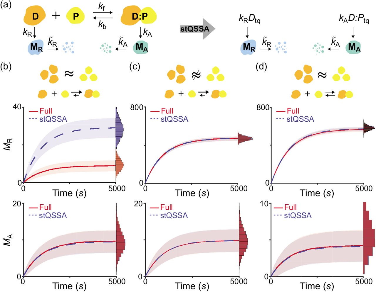
(a) Full model diagram of a gene regulatory network containing a rapid reversible binding between DNA (D) and a transcription factor (P) to form a complex (D:P) (left, Table S1). The transcription rates of MR and MA are proportional to D and D:P, respectively. By replacing D and D:P with their stQSSAs (Dtq and D:Ptq), we can obtain a reduced model which consists of only slowly varing MR and MA (right, Table S2). (b-d) Trajectories of MR (top) and MA (bottom) from the full model (red) and the reduced model (blue) simulated using the Gillespie algorithm (see Tables S1 and S2 for propensity functions). The lines with colored ranges and the histograms represent the mean ± standard deviation and the stationary distribution of 104 trajectories, respectively. When DT and PT are the same (DT = PT = 10) and the binding is tight (Kd = 10−2), the MR trajectories simulated with the reduced model largely exceed those simulated with the full model (b top) because Dtq overestimates the stochastic QSSA for D(〈D〉). On the other hand, D:Ptq accurately approximates the stochastic QSSA for D:P (〈D:P〉), and thus the reduced model accurately captures the dynamics of MA (b bottom). If DT is not similar to PT (DT = 15, PT = 10) (c) or the binding is weak (Kd = 10) (d), Dtq and D:Ptq accurately approximate 〈D〉 and 〈D:P〉, respectively, so that the reduced model accurately captures the dynamics of both MR and MA of the full model.
To test whether the reduced model accurately captures the dynamics of the full model, we compared their stochastic simulations with the Gillespie algorithm (see Tables S1 and S2 for propensity functions) [53]. When DT and PT are the same and the binding between D and P is tight, MR simulated with the reduced model largely exceeds MR simulated with the full model (Fig 2b top) because the stQSSA (Dtq) overestimates the stochastic QSSA for the number of the unbound DNA (〈D〉) which determines the transcription rate of MR (Fig 2a), as seen in Fig 1f. On the other hand, when DT is not similar to PT (Fig 2c top) or the binding is weak (Fig 2d top), Dtq accurately approximates 〈D〉 as seen in Fig 1d, and thus the reduced model accurately captures the dynamics of MR in the full model.
Unlike MR (Fig 2b top), the stochastic dynamics of MA of the reduced model and the full model are identical (Fig 2b–2d bottom) because the stQSSA for D:P (D:Ptq) always accurately approximates the stochastic QSSA for the number of the bound DNA (〈D:P〉) which determines the transcription of MA (Fig 1c). Taken together, the stQSSA can be used to describe transcriptional activation depending on bound DNA under any conditions (Fig 2b–2d bottom). On the other hand, it needs to be restrictively used to describe transcriptional repression depending on unbound DNA (Fig 2b–2d top).
stQSSA can distort oscillatory dynamics
To illustrate how the stQSSA distorts the dynamics when the molar ratio between tightly binding species is ~1:1, we investigated the simple model where the molar ratio is conserved (Fig 2). However, the molar ratio can be varied (e.g., oscillate) in a living cell due to other reactions in a larger system. This raises the question of whether the model reduction based on the stQSSA is accurate or not if the molar ratio is temporarily ~1:1. To investigate this, we used a modified Kim-Forger model, which describes the transcriptional negative feedback loop of the mammalian circadian clock [25,50,52]. In this model (Fig 3a top, Table S3), free activator (A) promotes the transcription of mRNA (M), and the protein translated from M produces repressor (R) passing through several steps (Pi, i = 1, 2, 3). Then R reversibly binds with A to form a complex (A:R) which no longer promotes the transcription, and thus represses its own transcription. In this model, the reversible binding between R and A is much faster than the other reactions (i.e., production and decay). Thus, by replacing the fast variable A, which determines the transcription rate of M, with its stQSSA (Atq), we can obtain a reduced model (Fig 3a bottom, Table S4). The reduced model consists of only the slow variables, RT, M and Pi, because Atq is fully determined by the conserved total number of the activator (AT = A + A:R) and the slowly varying total number of the repressor (RT = R + A:R), as illustrated in Table S4.
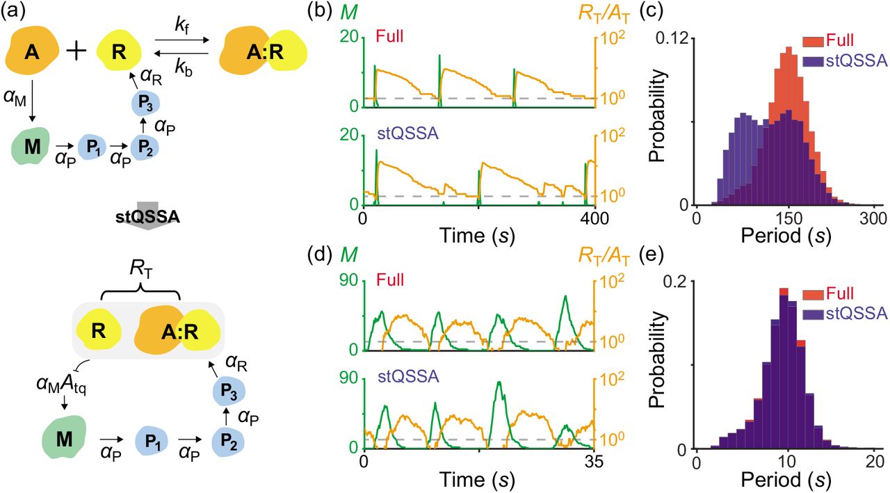
(a) Full model diagram of an oscillatory transcriptional negative feedback loop (top, Table S3). Unbound activator (A) promotes the transcription of mRNA (M), and the protein translated from M produces repressor (R) passing through several steps (Pi, i = 1, 2, 3). Then R binds with A to form a complex (A:R) which is transcriptionally inactive, and thus represses its own transcription. As the reversible binding between R and A is rapid, by replacing A with its stQSSA (Atq), we can obtain a reduced model which consists of only slowly varying RT, M, and Pi (bottom, Table S4). (b-c) Oscillatory trajectories of M (green) and RT/AT (orange) simulated with the full model (b top) and the reduced model (b bottom), using the Gillespie algorithm (see Tables S3 and S4 for propensity functions). When R binds with A tightly (Kd = 10−4) both the full model and the reduced model show the oscillatory behaviors. However, when the trajectory of RT/AT stays near 1 (dashed lines in b), Atq overestimates the stochastic QSSA for A(〈A〉), and thus the transcription more frequently occurs in the reduced model (b bottom) compared to the full model (b top). As a result, the reduced model predicts a shorter period than the full model (c). (d-e) On the other hand, when the degradation rate of R increases and thus the trajectory of RT/AT stays near 1 for a short time (d; dashed lines), the reduced model accurately captures the dynamics of the full model (e).
In the model, because R tightly binds with A, when RT/AT ≈ 1, Atq overestimates the stochastic QSSA for A (〈A〉) and thus the transcription rate of M. As a result, when the trajectory of RT/AT reaches close to 1 (dashed lines in Fig 3b), the transcription more frequently occurs in the reduced model (Fig 3b bottom) compared to the full model (Fig 3b top). This overestimated transcriptional activity leads to the shorter peak-to-peak periods of the reduced model compared to the full model (Fig 3c). On the other hand, when the degradation rate of R increases and thus the trajectory of RT/AT stays near 1 for an extremely short time (Fig 3d dashed lines), the reduced model accurately captures the dynamics of the full model (Fig 3e). Taken together, if ~1:1 molar ratio between the tightly binding activator and repressor of the transcriptional negative feedback loop persists for a considerable time, using the stQSSA overestimates the transitional activity and thus the frequency of oscillation.
stQSSA can distort bistable dynamics
To investigate how the misuse of the stQSSA distorts the dynamics of a bistable switch, we used a previously developed bistable switch model for the maturation promoting factor, cyclin B/Cdc2, whose activation promotes mitosis (Fig 4a top, Table S5) [47,57]. In the model, the inactive form of cyclin B/Cdc2 (P) is converted to an active form (M) by Cdc25 (D). Furthermore, as M activates D which converts P to M, M promotes its own activation (i.e., form a positive feedback loop; see [47,57] for details). The positive feedback loop is suppressed by Suc1 protein (B) as it binds with M to form a complex (M:B) which no longer activates D. The total activated cyclin B/Cdc2 (M and M:B) become P with the same constant rate. In this model, the reversible binding between M and B is much faster than the other reactions. Thus, by replacing the fast variable M with its stQSSA (Mtq) a reduced model can be derived (Fig 4a bottom, Table S6). The reduced model consists of only the slow variables, MT and P, because Mtq is fully determined by the conserved total number of Suc1 (BT = B + M:B) and the slowly varying total number of the activated cyclin B/Cdc2 (MT = M + M:B), as illustrated in Table S6.

(a) Full model diagram of a bistable switch for mitosis (top, Table S5). The inactive form of cyclin B/Cdc2 (P) becomes an active form (M) by Cdc25 (D). In this process, M enhances its own activation by activating D, and thus forms a positive feedback loop (see [47,57] for details). The positive feedback loop is suppressed as Suc1 protein (B) binds with M to form a complex (M:B) which does not activates D. The total activated cyclin B/Cdc2, M and M:B, becomes P with the same constant rate. As the reversible binding between M and B is rapid, by replacing M with its stQSSA (Mtq), we can obtain a reduced model which consists of only slowly varying MT and P (bottom, Table S6). (b-c) Simulated trajectories (b) and the stationary distributions (c) of MT from the full model and the reduced model using the Gillespie algorithm (see Tables S5 and S6 for propensity functions). When M binds with B tightly (Kd = 10−3), both the full model and the reduced model show the bistable behaviors between the upper and lower modes, which are separated by MT/BT = 1 (dashed line in b). However, because Mtq overestimates the stochastic QSSA for M (〈M〉) when MT/BT is close to 1, the trajectory from the reduced model is more attracted to the upper mode compared to the full model (b). As a result, the bimodal distribution of MT from the reduced model is biased to the upper mode (c). (d-e) On the other hand, when the binding between M and B becomes weak (Kd = 10), Mtq accurately estimates 〈M〉, and thus the reduced model accurately captures the dynamics of the full model, which no longer shows the bistable behavior.
When M and B tightly bind, both the full model and the reduced model show the bistable behaviors (i.e., bimodal stationary distributions) of MT (Fig 4b). However, the trajectory of the reduced model is more attracted to the upper mode of MT compared to the full model (Fig 4b and 4c). This dynamics biased to the upper mode occurs because Mtq overestimates the stochastic QSSA for M(〈M〉) near the MT/BT = 1 region (Fig 4b dashed line) which separates the upper and lower modes. On the other hand, when the binding between M and B becomes weak, Mtq accurately approximates the stochastic QSSA for M even when MT is similar to BT. Thus, the reduced model accurately captures the dynamics of the full model, which no longer shows bistable behavior (Fig 4d and 4e). Taken together, when the binding between activated Cyclin B/Cdc2 and Suc1 protein is tight, which is essential to generate the bistable switch, using the stQSSA overestimates the activation of Cyclin B/Cdc2 and distorts the dynamics of the bistable switch.
An alternative approach when the stQSSA is not applicable
In the presence of a rapid and tight reversible binding between species whose molar ratio is ~1:1, the reduction of stochastic models with the stQSSA for the number of the unbound species can cause errors (Figs 2b, 3c, and 4c). In such cases, due to the tight binding, the two species tend to bind until no molecules of one species left (Fig 1f). Specifically, if AT ≤ BT (AT ≥ BT), the majority of the A (B) will be bound. Thus, in the presence of tight binding, we can assume that the stationary distributions of A or B are concentrated on 0 and 1. This low-state assumption allows us to derive the simple approximation for the stochastic QSSA (〈A〉 in Eq. (4)) (see Methods for details):

We will refer to this approximation as the stochastic “low-state” QSSA (slQSSA).
The accuracy of the slQSSA for A (Eq. (9)) is expected to increase when ATKd decreases because ATKd is an approximated number of the unbound A. On the other hand, the accuracy of the stQSSA for A decreases as ATKd decreases (Fig 1d). To investigate this, we calculated the maximum relative error of  and
and  to the stochastic QSSA for A(〈A〉) for each ATKd and Kd (Fig 5a and 5b). As expected, when ATKd is low and high, the slQSSA and the stQSSA are accurate, respectively. In particular, when ATKd < 10−1 and ATKd > 101,
  and RA are less than 0.1 (i.e., the relative errors are less than 10%), respectively.
The parameters used in Figs 2b (triangle), 3b (circle), and 4b (square) are located in the region where the stQSSA is inaccurate (Fig 5a) but the slQSSA is accurate (Fig 5b). Therefore, with these parameters, the reduced models obtained by using the slQSSAs accurately capture the dynamics of the full models for the simple gene regulatory network (Fig 5c, Table S2), the transcriptional negative feedback loop (Fig 5d, Table S4), and the bistable switch for mitosis (Fig 5e, Table S6), unlike the stQSSA (Figs 2b, 3c, and 4c). Furthermore, by allowing A or B to reach more than two states (e.g., 0, 1, and 2), more accurate slQSSAs can be derived (see Methods for details). In particular, the relative errors of the slQSSAs derived by allowing the 3/4/5 states are less than 0.1 when ATKd is less than 2/5/10, respectively (Fig S2). Consequently, if ATKd < 101 and thus the stQSSA is inaccurate, the slQSSA can be used to approximate the stochastic QSSA for A (Fig 5f). Taken together, by using either stQSSA or slQSSA depending on ATKd, we can always accurately reduce multiscale stochastic biochemical systems with rapid reversible bindings.

(a-b) Heat maps of the relative errors ( and
and  ) when the stQSSA (Atq) and the two-state slQSSA (Alq) approximate the stochastic QSSA for A (〈A〉) in the reversible binding reaction (Eq. (1)). Color represents the maximum value of RA and
  for each ATKd and Kd when BT varies, and the dashed lines represent when those values are 0.1. When ATKd are high and low, the stQSSA and the slQSSA are accurate, respectively. The parameters used in Figs 2b (triangle), 3b (circle), and 4b (square) are located in the region where the slQSSA (b), but not the stQSSA (a), is accurate (the circle is actually located outside of the heat maps; ATKd = 5 × 10⁻⁴ and Kd = 10−4). (c-e) As a result, the full models are successfully reduced with the slQSSA (c-e) but not the stQSSA (Figs 2b, 3c, and 4c). See Tables S2, S4, and S6 for the propensity functions used for the simulations. (f) The adaptive use of the stQSSA and the slQSSA to approximate the stochastic QSSA for A when ATKd > 101 and otherwise, respectively, guarantees the successful reduction of stochastic models containing rapid reversible bindings. Note that when 10−1 < ATKd < 101, the slQSSAs with more than two states need to be used (see Fig S2 for details).
Discussion
Reversible binding between molecules—for example, between DNA and a transcription factor, a ligand and a receptor, and an enzyme and a substrate—is a fundamental reaction for numerous biological functions [43]. As the reversible binding reactions occur typically on a timescale of 1 ~ 1000ms, which is much faster than the other reactions (e.g., 30min for a mammalian mRNA transcription or a protein translation and 10h for their typical lifetimes) [44], a system containing the rapid reversible binding becomes a multi-timescale system. In such multi-timescale systems, the rapid reversible binding prohibitively increases the computational cost of stochastic simulations. Accordingly, to accelerate stochastic simulations, various methods have been developed [45, 58]. In particular, the model reduction using the stQSSA has successfully simplified various stochastic models in numerous studies [7,31–34,39,40]. Thus, it has been commonly believed that the stQSSA is generally accurate for any conditions, until a recent counterexample was identified [42]. In this work, we rigorously derived the validity conditions for using the stQSSA to reduce stochastic models with a rapid reversible binding. Specifically, we showed that the relative error of the stQSSA for the number of unbound species (RA) mainly depends on the relative sensitivity of the stQSSA (SA, Eq. (8)), which attains maximum value  at AT = BT + Kd. This allowed us to find that the stQSSA for the number of the unbound species is inaccurate if their molar ratio is ~1:1 and their binding is tight (Fig 1f). In that case, the stQSSA highly overestimates the number of the unbound species. Therefore, the reduced models obtained by using the stQSSA distort the dynamics of the gene regulatory model (Fig 2b), the transcriptional negative feedback loop model for circadian rhythms (Fig 3c), and the bistable switch model for mitosis (Fig 4c).
Interestingly, even in the invalid range of the stQSSA, identified in this study, the deterministic tQSSA is known to be accurate [7, 49, 51]. Indeed, for all examples considered in our work (Figs 2b, 3b, and 4b), the deterministic simulations with the tQSSA are accurate, unlike the stochastic simulations. This indicates that it is risky to investigate the validity conditions of the stQSSA solely based on the validity conditions of the deterministic tQSSA. Instead, direct derivation of the relative error of the stQSSA is needed as demonstrated in this study (Eq. (7)). It would be interesting in future work to perform such error analysis for more complex examples, such as coupled enzymatic networks with multiple rapid reversible bindings [27, 59, 60].
While the deterministic tQSSA (Eq. (3)) was used to approximate the stochastic QSSA for the number of reversibly binding species in this work, a simpler deterministic QSSA referred to as the “standard” QSSA (sQSSA) is more widely used to approximate the stochastic QSSA due to its simplicity [8–21,28,33]. For instance, the stochastic sQSSA for C in Eq. (1), which has the Michaelis-Menten type form:
 has been widely used as a propensity function for Gillespie algorithm. However, it is less accurate than the stQSSA (Eq. (5)) [39, 40]. This is why many examples showing the inaccuracy of the stochastic sQSSA have been reported [34–41], whereas only one example showing the inaccuracy of the stQSSA has been reported [42]. Importantly, our work also provides the validity condition for using the stochastic sQSSA (Eq. (10)). That is, when BT + Kd ≫ AT, which is known as the low-enzyme concentration condition, Csq ≈ Ctq [7], indicating that the Michaelis-Menten type sQSSA for the bounded species (Eq. (10)) can be used to reduce models containing the rapid reversible binding. Similarly, when BT + Kd ≫ AT,
  could also be used. This is consistent with the validity conditions for the stochastic sQSSA derived under the assumption of either low fluctuation level [33] or low copy number [41]. Furthermore, the “pre-factor” QSSA (pQSSA), which is more accurate than the sQSSA, has also been used for stochastic simulations [61,62]. However, recent studies have shown that the stQSSA is more accurate than the stochastic pQSSA (see [39, 40] for details).
The accuracy of the stQSSA for the number of the unbound species depends on both the molar ratio between reversibly binding species and the tightness of their binding (Fig 1d). However, as the molar ratio typically varies in larger models containing reversible binding, practically, the accuracy is mainly determined by the tightness of binding. Specifically, for the relative error of the stQSSA to be less than 0.1, ATKd (≈ the number of the unbound A) should be larger than 10 (Fig 5a dashed line). This ATKd value-based criteria explains the controversy about the accuracy of the stQSSA in previous studies. That is, ATKd was less than 10 in a previous study where the reduced model obtained by using the stQSSA was inaccurate [42]. On the other hand, ATKd were much greater than 10 in all of the examples investigated in previous studies reporting the accuracy of the stQSSA [7,34,39,40,54,55]. Furthermore, the stQSSA always accurately approximates the stochastic QSSA for the number of the bound species (Fig 1c). This explains why the stQSSA was accurate in previous studies where the stQSSA was used to approximate the number of enzyme-substrate complex [31–34].
In real biological systems, the validity condition for the stQSSA for the number of the unbound species (ATKd > 10) is not always guaranteed. Specifically, the range of ATKd can span approximately from 10−2 to 1010 since the volume of the human cells is 10−15 ~ 10−14m3, the protein-protein dissociation constant is 10fM ~ 1μM (i.e., 1012 ~ 1020m−3), and the numbers of molecules is 100 ~ 104 [44,63]. Accordingly, as an alternative for the stQSSA, we derived the slQSSA, which accurately approximates the stochastic QSSA when ATKd is less than 10. Specifically, the relative error of the slQSSA, unlike that of the stQSSA (Fig 5a and 5b), decreases as ATKd decreases because the slQSSA relies on the assumption that the stationary distributions of the number of the unbound species (≈ ATKd) are concentrated on the few lowest states. Taken together, by using the stQSSA and the slQSSA when the ATKd value is greater and less than 10, respectively, one can always accurately simplify stochastic models containing rapid reversible binding reactions to accelerate simulation and also facilitate stochastic analysis (Fig 5f).
Methods
Exact bounds for the relative error of the stQSSA to the stochastic QSSA
In this section, we derive the exact upper and lower bounds for  (Eq. (7)) where Atq and 〈A〉 are the stQSSA and the stochastic QSSA for A, respectively. From the CME describing the reversible binding reaction (Eq. (1)), the following steady-state moment equation can be derived:
 where 〈·〉 is the stationary expectation. Eq. (11) becomes 〈A · (BT – AT + A)〉 = Kd〈AT – A〉 by using the definitions AT = A + C, BT = B + C, and Kd = kbΩ/kf. Since AT and BT are invariant under the reversible binding reactions in Eq. (1), we obtain 〈A2〉 – (AT – BT – Kd)〈A〉 – ATKd = 0, and by using the relation 〈A2〉 = Var(A) + 〈A〉2, we get the following quadratic equation:

The non-negative root of this quadratic equation becomes 〈A〉:

By subtracting Eq. (13) from Eq. (5), we get


Since 0 ≤ (AT – BT – Kd)2 + 4ATKd – 4Var(A) ≤ (AT – BT – Kd)2 + 4ATKd, we get the bounds for Atq – 〈A〉 from Eq. (15):

By dividing Eq. (16) by 〈A〉, we can get the bounds for the relative error,  as follows:

This can be re-expressed as FASA ≤ RA ≤ 2FASA (Eq. (7)) because  is the Fano factor of A (FA), and
  is the relative sensitivity of Atq, i.e.,
  .
.
The relative sensitivity, SA, attains the maximum value  when the term in the square root of the denominator has the minimum value, i.e., BT = AT – Kd (Eq. (8)). In particular, SA has a large maximum value when Kd ≪ 1 at AT = BT + Kd ≈ BT. On the other hand, if AT ≪ BT, SA ≈ 0 because the majority of A presents in the bound state regardless of BT (i.e.,
  ). When AT ≥ BT,
  because as BT decreases by one, approximately one A is released from the complex. In this case, if AT ≫ BT, the majority of A are free and thus
  , leading to SA ≈ 0. However, if AT ≈ BT, the majority of A is sequestered by B, Atq ≈ 0, leading to SA ≫ 1. When binding is weak (Kd ≫ 1), SA ≈ 0 because the number of A, which is approximated by Atq, changes little as BT changes (i.e.,
  ). Taken together, SA is large only when the binding reaction is tight (Kd ≪ 1) and the binding species are present with 1:1 molar ratio (AT ≈ BT).
Derivation of the stochastic QSSA and the slQSSA
Here we derive the stochastic QSSA for A (〈A〉, Eq. (4)). Let p(l) be the probability that A = l at its stationary distribution (i.e., the probability that A(∞) = l). Then the following recurrence relation of p(l) can be obtained from the steady-state CME:

Let A0 = max{AT – BT, 0}. Since A0 is the lowest state that A can reach, p(l) = 0 for l < A0. Then we can inductively prove that the following relation satisfies Eq. (17):
 where
where  . Then, because Σp(l) = 1,
  if A0 ≤ l ≤ AT, and p(l) = 0 otherwise by Eq. (18). Therefore, we can obtain the stationary average number of A (Eq. (4)) as

Next we derive the slQSSA, which is the approximation for Eq. (4). In the presence of tight binding, we can assume that the stationary distributions of A and B are concentrated on the states {0,1} when AT < BT and AT ≥ BT, respectively. Since when the distribution of B is concentrated on 0 and 1, the distribution of A is concentrated on AT – BT and AT – BT + 1, we can simply say that the distribution of A is concentrated on A0 and A0 + 1. Thus, by assuming that  is approximately zero for l > A0 + 1 and
  , we can derive the two-state slQSSA for A (Eq. (9)) as follows:

In general, for any integer k ≥ 2, we can derive the k-state slQSSA as

We provide a Matlab code, LQSSA, that can be used to calculate Eq. (19).
Supporting information
S1 Appendix. Supplementary Methods, Tables S1-S6, and Figs S1-S2. (PDF)
S1 File. LQSSA (M)
Author Contributions
All authors designed the study and performed mathematical analysis. YS performed the computation and all authors analyzed the computation results. YS and JKK wrote the draft and all authors revised the manuscript.
Acknowledgments
We thank Krešimir Josić and John J. Tyson for valuable comments. This work was funded by NRF-2016 RICIB 3008468 (JKK), the Institute for Basic Science IBS-R029-C3 (JKK), and NRF-2019-Fostering Core Leaders of the Future Basic Science Program/Global Ph.D. Fellowship Program 2019H1A2A1075303 (HH).
Footnotes
Discussion section has been revised.
References


