

ABSTRACT
Polygenic scores have become the workhorse for empirical analyses in social-science genetics. Because a polygenic score is constructed using the results of finite-sample Genome-Wide Association Studies (GWASs), it is a noisy approximation of the true latent genetic predisposition to a certain trait. The conventional way of boosting the predictive power of polygenic scores is to increase the GWAS sample size by meta-analyzing GWAS results of multiple cohorts. In this paper we challenge this convention. Through simulations, we show that Instrumental Variable (IV) regression using two polygenic scores from independent GWAS samples outperforms the typical Ordinary Least Squares (OLS) model employing a single meta-analysis based polygenic score in terms of bias, root mean squared error, and statistical power. We verify the empirical validity of these simulations by predicting educational attainment (EA) and height in a sample of siblings from the UK Biobank. We show that IV regression between-families approaches the SNP-based heritabilities, while compared to meta-analysis applying IV regression within-families provides a tighter lower bound on the direct genetic effect. IV estimation improves the predictive power of polygenic scores by 12% (height) to 22% (EA). Our findings suggest that measurement error is a key explanation for hidden heritability (i.e., the difference between SNP-based and GWAS-based heritability), and that it can be overcome using IV regression. We derive the practical rule of thumb that IV outperforms OLS when the correlation between the two polygenic scores used in IV regression is larger than  , with N the sample size of the prediction sample.
Introduction
Genome-Wide Association Studies (GWASs) have been successfully used to analyze the genetic architecture of various diseases and human traits (1). These GWASs have firmly established that, with few exceptions, most human (behavioral) traits are highly “polygenic” – that is, influenced by many individual genetic variants, each with a very small effect size (the “Fourth Law” of behavior genetics; 2). A natural consequence of this finding has been the widespread adoption of so-called polygenic scores (PGSs), weighted sums aggregating the small effects of numerous genetic variants (single-nucleotide polymorphisms; SNPs), which enable out-of-sample genetic prediction of complex traits (3; 4; 5). However, an estimated PGS is a noisy proxy for the true (latent) PGS because, amongst other reasons, the GWAS underlying the construction of the PGS is based on a finite sample (6).
It is common practice to meta-analyze GWAS summary statistics from as many cohorts as possible to foster the identification of genome-wide significant SNPs (1). Through the law of large numbers, this strategy has also proven to be very effective in reducing measurement error in the PGS and thus to boost power for genetic prediction (4). PGSs are now able to explain a non-negligible proportion of the variance in health and behavioral traits. Nevertheless, the predictive power of today’s PGSs is still substantially smaller than the SNP-based heritability estimates. The SNP-based heritability can be obtained using Linkage Disequilibrium (LD)-score regression (LDSC; 7) or Genome-based Restricted Maximum Likelihood (GREML; 8) and constitutes an upper bound for the predictive power of PGSs (9).1 For example, the current maximum predictive power, or variance explained in the phenotype (R2), of the educational attainment (EA) PGS is about 12% (11) whereas the SNP-based heritability is estimated to be in the range 22-28% (e.g., 12; 13; 14). This difference between the SNP-based and GWAS-based heritability is referred to as ‘hidden heritability’ (e.g., 10).2
Uncovering the ‘hidden heritability’ and reaching the upper bound of the SNP-based heritability using PGSs is important for multiple reasons. First, measurement error in the PGS reduces statistical power. With less noisy PGSs, it will be easier to detect currently unknown genetic correlations, to analyze possible gene-by-environment (G × E) interactions, and to reduce omitted variable bias concerns when PGSs are used as control variables. Second, measurement error in the PGS may lead to misclassification in personalized medicine and screening decisions. For example, when screening for cardiovascular disease is partly based upon values of the PGS (e.g., 15), measurement error in the PGS may lead to some individuals being erroneously left out of screening procedures whereas others are erroneously included (e.g., 16).
The expected predictive power of a PGS in terms of the explained phenotypic variance explained in a linear regression model is given by (17; 18):  , where
  denotes the SNP-based heritability, M ~ 70, 000 is a population-genetic parameter corresponding to the number of effective loci (19), and N the discovery sample size. Figure 1 shows the relation between the predicted R2 and the discovery sample size N, assuming a SNP-based heritability
  (corresponding to the phenotype height, (20; 21)), and
  (the mid-point of the range 22-28% estimated for EA (e.g., 12; 13; 14)). The figure shows that there are significant diminishing returns to further increases in GWAS sample size. Whereas the predictive power of the PGS increases rapidly with the sample size when going from a (meta-analyzed) discovery sample size of a few thousands to a sample of around 1 million individuals, the returns to sample size in terms of predictive power decrease for larger samples. For EA, it takes a sample of ~1 million to construct a PGS explaining 0.20, but it would take a 7-fold increase in discovery sample size to achieve an R2 of 0.24.3

Predicted R-squared (variance explained) versus the sample size of the discovery sample in the GWAS for height (SNP-based heritability around 0.50) and EA (SNP-based heritability around 0.25).
In this paper, we use analytical derivations, simulations, and empirical data, to derive the conditions under which an Instrumental Variable (IV) approach outperforms the convention of meta-analysis. We build upon and extend the approach developed by DiPrete et al. (19), who first suggested the IV approach to reduce measurement error in the PGS as a by-product of their Genetic Instrumental Variable (GIV) method. The intuition of the IV approach is to split the GWAS discovery sample to obtain two PGSs that both proxy the same underlying ‘true’ PGS. Since the measurement error in the two PGSs is plausibly independent, we will refer to these PGSs as ‘independent’ PGSs. In the case of no measurement error, theoretically the correlation between the two PGSs should approach 1. The IV approach then infers the amount of measurement error through the empirical correlation between the two independent PGSs, and in turn uses this information to correct (or ‘scale’) the observed association between the PGS and the phenotype.
Our contribution over (19) is threefold. First, we analytically derive an alternative way to standardize an estimated PGS to estimate a consistent standardized effect of the true latent PGS on the phenotype when using IV. This standardization ensures that the square of the standardized effect can be interpreted as the GWAS-based heritability without further ex post correction. Second, we avoid the arbitrary choice of selecting one PGS as the independent variable and the other as IV by using the recently developed Obviously-Related Instrumental Variables (ORIV) technique (22). Third, and arguably foremost, we establish the conditions and a practical rule of thumb under which our ORIV estimator outperforms a meta-analysis PGS in terms of (i) bias, (ii) root mean squared error (RMSE), and (iii) statistical power.
Due to an increase in the number of cohorts releasing GWAS summary statistics sufficiently precise to compute PGSs with non-negligible predictive power, we believe our contribution to be very timely. For example, as we demonstrate in this paper, the sample sizes of the UK Biobank (UKB) and the 23andMe, Inc. are individually large enough to generate a PGS for EA with a predictive power of 5% (23andMe) to 7% (UKB). The main contribution of this paper is then to answer a simple question: what should an applied researcher do to maximize the predictive power of the PGS? Meta-analyze the GWAS summary statistics from UKB and 23andMe to construct a single PGS, or apply ORIV using two independently constructed PGSs? We reach three main conclusions in our study.
First, when the prediction sample is sufficiently large, the genetic correlation between the discovery samples is close to 1, and the correlation between the independent PGSs is not too low, then ORIV outperforms meta-analysis in terms of bias, root mean squared error (RMSE), and power. More specifically, ORIV outperforms meta-analysis when
 where N denotes the sample size of the prediction sample, F* denotes a given target value of the F-statistic in the first stage of the ORIV regression, and PGS1 and PGS2 denote the independently constructed PGSs. The intuition is that ORIV provides consistent, yet biased estimates, with the bias of ORIV inversely proportional to the first-stage F-statistic (e.g., 23; 24). The first stage in this context is a regression of one PGS on the other, and – since the PGSs are typically standardized to have mean 0 and standard deviation 1 – it simply reflects the correlation between the two PGSs. As a result, the performance of ORIV depends on the correlation between the two independent PGSs, and on the sample size of the prediction sample. Using a simulation study that is calibrated on the empirical predictive power of the PGSs for EA, our results suggest that the commonly used Staiger and Stock (24) threshold of F* = 10 also applies here. Therefore, equation (1) with F* = 10 provides a practical rule-of-thumb when ORIV outperforms meta-analysis in terms of lower bias, lower RMSE, and higher statistical power. That is, after rearranging terms of equation (1), when
  .
.
Second, our simulations show that the application of ORIV in a between-family setting results in the unbiased estimation of SNP-based heritability when all assumptions are satisfied.4 Our empirical illustration using EA in the UK Biobank sibling sample shows that applying ORIV in a between-family design increases the estimated GWAS-heritability from 0.076 (s.e. 0.003) to 0.114 (s.e. 0.004). This estimated GWAS-heritability is somewhat below most SNP-based heritability estimates reported in the literature, but in our sample the SNP-based heritability for EA is estimated to be 0.155 (s.e. 0.019) using GREML and 0.160 (s.e. 0.028) using LDSC. In other words, ORIV recovers a substantial portion of the SNP-based heritability. Similar conclusions can be drawn for body height with the estimated GWAS-heritability rising from 0.340 (s.e. 0.006) (OLS) to 0.426 (s.e. 0.008) (ORIV), and with the SNP-based heritability estimated as 0.530 (s.e. 0.020) using GREML and 0.511 (s.e. 0.041) using LDSC. Hence, we empirically confirm that the ORIV estimates more closely approximate the SNP-based heritability than OLS estimates on basis of a meta-analysis based PGS.
Third, we find that applying ORIV in within-family designs provides a tighter lower-bound on the ‘direct’ genetic effect compared with OLS using a meta-analysis based PGS. Within-family estimates are the gold standard for estimating direct genetic effects (i.e., estimates free from bias due to genetic nurture and population stratification, see e.g., (25)). This is because the variation in genotypes across siblings is randomly assigned at conception according to Mendel’s First Law. However, as we explain in the Methods section, when using PGSs to uncover direct genetic effects, within-family estimates are downward biased due to measurement error in the PGS, genetic nurture (26), and social genetic effects (27; 28). As a result, within-family estimates of the effect of the PGS on an outcome constitute a clear lower bound on the direct genetic effect. While the bias due to genetic nurture and social genetic effects can only be overcome by controlling for parental genotype in the discovery GWAS, random measurement error can be overcome by ORIV. Therefore, applying ORIV in a within-family design is currently the best way to estimate a tight lower bound on the direct genetic effect.5 In our empirical applications in the UKB, our within-family IV estimates are respectively 30% (EA) and 14% (height) higher than the effect sizes obtained using meta-analysis. Moreover, it also allows estimating a lower bound on the ‘direct GWAS-based heritability’, that is, the contribution of SNPs to variation in the outcomes net of indirect genetic effects such as genetic nurture. In our data, we are able to increase this lower bound for EA from 2.0% to 3.4%, and for height from 28.9% to 37.7%.
Results
Simulation study
Our simulation compares the performance of meta-analysis and ORIV in estimating the standardized effect of the PGS on an outcome variable. We vary the sample size of the prediction sample and the measurement error in the PGSs. The simulations are calibrated based on educational attainment (EA), but we show that our conclusions hold for other complex traits at varying levels of heritability. The SNP-based heritability serves as the natural upper bound for the R2 of the PGS (9), which is approximately equal to 25% for EA in most samples (12; 13; 14). This corresponds to a correlation coefficient of 0.5 between the PGS and the outcome (i.e., the square root of the incremental R2). Hence, we assume that the standardized outcome EA and the standardized true latent PGS* are drawn from a bivariate standard normal distribution with correlation 0.5.
In practice, the true (latent) PGS* is not observed, and we have to work with approximations of the latent PGS that suffer from measurement error. In particular, we assume that an estimated PGS is equal to the true latent PGS* plus some additive classical measurement error ν (following, e.g., 30):
 with
with  . In order to model a realistic variance for the measurement error
  , we calibrate the simulations based on the predictive power of existing PGSs for EA. Based on the attenuation bias arising from measurement error in a linear regression of the outcome on the PGS, we can derive that (see equation 14 in the Methods section for a derivation):
 where
where  is the variance of the true latent PGS, βst is the true standardized coefficient (the coefficient resulting from a regression in which both the dependent variable and the true PGS are standardized to have mean 0 and standard deviation 1), and
  is an estimated standardized coefficient from the literature. We derive the ‘true’ βst from the square root of the SNP-based heritability estimate, and we infer
  from the square root from an estimated incremental R2 in the literature.6 In the simulations, we set the true standardized effect size to βst = 0.5 and
  . These choices are however largely inconsequential, because we derive in the Methods section that the bias of both OLS (meta-analysis) and ORIV depends on the ratio

In words, the performance of OLS and ORIV is determined by how closely the estimated GWAS-based heritability on basis of a given PGS (i.e., the square of the estimated standardized effect) approximates the SNP-based heritability  . We coin this term the “explained SNP-based heritability”. Even though we analytically show that the performance of OLS and ORIV depends on the ratio of coefficients rather than on the absolute values, in the Appendix we investigate the sensitivity of our results with respect to absolute values of βst and
  .
.
In each simulation trial, we generate a ‘meta-analysis PGS’ with  , corresponding to an incremental R2 of 12% as in the third and latest GWAS on EA (11), and corresponding to an explained SNP-based heritability of
  . In addition, to allow for the ORIV estimation, we construct two independent PGSs. In order to make a fair comparison, we simulate the two independent PGSs with a lower predictive power than the meta-analysis PGS has. More specifically, we sequentially simulate two independent PGSs, each with values
  (corresponding to the incremental R2 of ~ 7.0% that we obtain based on our own GWAS in UKB),
  (corresponding to the incremental R2 of 3.2% as in the second GWAS of EA (13)), and
  (corresponding to the R2 of ~ 2% found in the first GWAS on EA (31)). We run 1,000 replications of the above simulation set-up, each time performing (i) a linear regression of the outcome on the meta-analysis PGS, and (ii) Obviously-Related Instrumental Variables (ORIV) estimation using the two independent PGSs as instruments for each other. We refer to the Methods section for details on the estimation. The sample sizes of the prediction sample we investigate are 1,000, 2,000, 3,000, 4,000, 5,000, 10,000 and 20,000.
The performance indicators we use are:
The relative bias of the estimator, defined by
 .
.The Root Mean Squared Error (RMSE), defined by
, which can be decomposed as the sum of the variance of the estimated and the squared bias.Statistical power, defined as the probability that the test rejects the null hypothesis when the alternative hypothesis is true. Given that our data-generating process simulates a non-zero standardized effect size, we report the fraction of replications in which we correctly reject the null hypothesis of a zero standardized effect (the empirical power).


The relative bias of the estimator is our first performance indicator, because meta-analysis will produce biased estimators by construction. However, so does IV with the bias in IV being inversely proportional to the first-stage F-statistic (23; 32). As we derive in the Methods section, in this context, the first stage F-statistic is given by (see equation 27 for a derivation):

We therefore analyze the relative bias of the two approaches when the sample size and correlation between the PGSs varies. The correlation between the two PGSs, which we denote by ρ, is determined by how closely the independent PGSs approximate the true PGS (i.e., the explained SNP-based heritability, see equations 15 and 17 in the Methods section). Therefore, even though we choose to present our results mainly in terms of correlation between the two independent PGSs (a value which is easy to compute in practice), the results can easily be translated in terms of the explained SNP-based heritability.
Apart from bias, we also study RMSE and statistical power. We do this because standard errors in Two-Stage Least Squares regression (the tool for IV estimation) tend to be larger than in Ordinary Least Squares regression (the tool for meta-analysis) even in larger samples where IV produces consistent estimates. Hence, for a fair comparison, we additionally study the RSME and statistical power. These two performance indicators both reflect bias as well as precision.
Figures 2a-2d depict our first set of simulation results, comparing meta-analysis and ORIV in terms of relative bias (top left, 2a), RMSE (top right, 2b), and statistical power (bottom left, 2c) for prediction sample sizes varying from 1,000 to 20,000 individuals. In these figures, the meta-analysis results are calibrated using the EA3 GWAS results (incremental R2 ~ 12%). We iteratively reduce the correlation ρ between the two independent PGSs used in ORIV estimation from 25% (corresponding to the R-squared of 7% we obtain based on our own UKB GWAS results) to 8% (corresponding to an R-squared of 2% as found in the EA1 GWAS). We maintain the same predictive power across the two independent PGSs. In the bottom-right panel, we present the average first-stage F-statistics for the three ORIV estimations (2d).

Relative bias, Root Mean Squared Error (RMSE), Statistical power, and first-stage F-statistic for meta-analysis (OLS) and ORIV for varying correlations (ρ) between the ‘independent’ PGSs. The simulation results are based on 1,000 replications.
In terms of bias, it is clear that ORIV outperforms meta-analysis. With relatively strong predictive power of the independent PGSs, ORIV produces estimates with very little bias even in relatively small prediction samples of only 1,000 individuals. In contrast, irrespective of the prediction sample size, meta-analysis substantially underestimates the effect. It bears repeating that simply increasing the sample size of the prediction sample will not help to overcome the attenuation bias of the meta-analyzed score (22; 33). In contrast, equation (5) and Figure 2a show that the bias of IV shrinks when the size of the prediction sample increases. This difference in bias between the estimators is to be expected, and so it is informative to additionally study performance measures that take into account precision. Here, a slightly more nuanced picture emerges. When the correlation between the two independent PGSs is only 0.08 – corresponding to a prediction R2 of around 2% and an explained SNP-based heritability of 8% – and the prediction sample has fewer than ~5,000 individuals, then the RMSE is lower and statistical power is higher in OLS (meta-analysis) than in ORIV. Whenever the prediction sample is beyond 5,000 individuals and the correlation between the independent PGSs is beyond 8%, then ORIV always outperforms meta-analysis in terms of all our statistical criteria with the difference increasing when the prediction sample size grows. Interestingly, these cases correspond roughly to the first-stage F-statistic being above 10 (bottom horizontal line in Figure 2d), a well-known rule of thumb in the IV literature (24).
A central assumption of the ORIV estimation is that the relative variance of measurement error is the same for each PGS (see the Methods section for more details), and that the genetic correlation between the two discovery samples is equal to one. This assumption is likely to be satisfied when the GWAS discovery sample is randomly split into two equally sized parts (19). It may be less likely to hold in case the PGSs are constructed using non-equally sized GWAS discovery samples stemming from different environments (e.g., countries). Therefore, in Figures 3a-3d we investigate the performance of meta-analysis and ORIV for the case where the meta-analysis PGS remains predictive at a R2 = 12%, but where the first independent PGS has a predictive power of R2 = 7% (corresponding to the PGS based on our own GWAS in UKB), and the second independent PGS has an R2 of either 5% (corresponding to the predictive power of the 23andMe PGS) or 2% (corresponding to the predictive power of the EA2 score (13)).
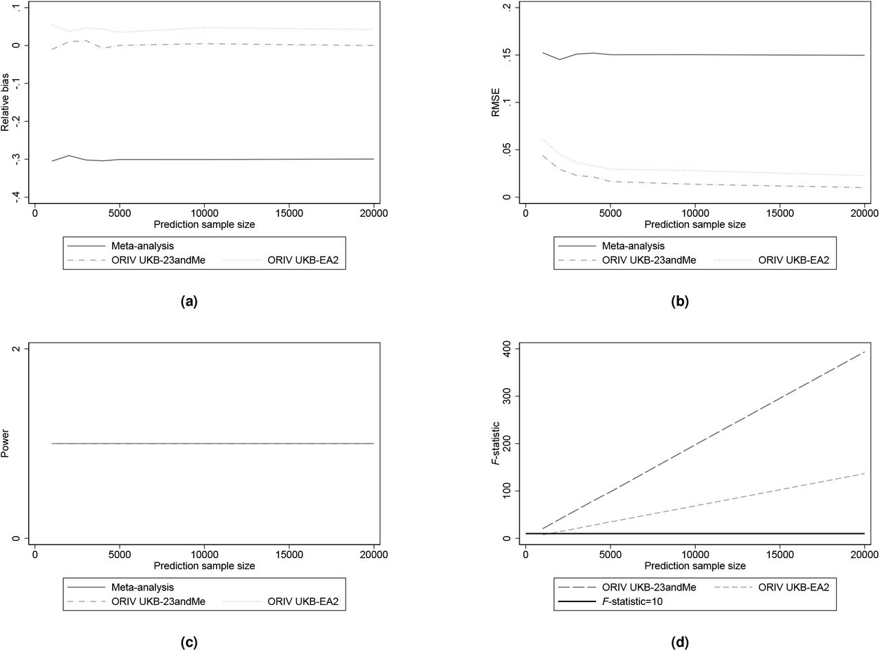
Relative bias, Root Mean Squared Error (RMSE), Statistical power, and first-stage F-statistic for meta-analysis (OLS) and ORIV with varying predictive power of the ‘independent’ PGSs used in ORIV. The simulation results are based on 1,000 replications.
Figures 3a and 3b show the bias and RMSE. When there is a substantial difference in predictive power across two independent PGSs – e.g., one PGS with R2 = 7%, and the other with R2 = 2% – a modest bias in the IV estimates remains, since the assumption of equal measurement error variance is not satisfied. Still, however, the bias and the RMSE of the IV estimates are relatively low when compared with the OLS meta-analysis results. Statistical power is identical for the two methods. We therefore conclude that ORIV estimation is not very sensitive to small violations of the assumption that the measurement error should have equal variance across the two independent PGSs. In the Appendix, we further vary the arbitrary chosen values of βst and σPGS*, and we show that our conclusions are not affected. In fact, consistent with our analytical derivations, the bias of meta-analysis depends largely on the explained SNP-based heritability rather than the absolute value of βst (see equation 4), and the performance of ORIV depends largely on the correlation between the two PGSs and the prediction sample size. Hence, it is not surprising that the absolute values of βst and σPGS* do not play a major role.
In sum, when plugging in the threshold value of F* = 10 and rearranging terms in equation (5), a reasonable rule of thumb on basis of these simulations is that ORIV outperforms meta-analysis whenever  . To provide some more feeling for what this rule of thumb implies, in a relatively large sample of 20,000 individuals the correlation between the two independent PGSs should exceed 0.02. In a modest sample of 1,000 individuals, the correlation between the two independent PGSs should be at least 0.10. Since the correlation between the two PGSs is equivalent to the explained SNP-based heritability of the two independent PGSs, this same rule of thumb can also be directly interpreted in terms of the explained SNP-based heritability of the independent PGSs.
Empirical illustration
In this section, we use OLS (meta-analysis) and ORIV to predict EA and height using PGSs in a subsample of European ancestry siblings in the UK Biobank (N = 35,282). We first residualized the outcomes EA and height for sex, year of birth, month of birth, sex interacted with year of birth, and the first 40 principal components of the genetic relationship matrix. More details on the variables and their construction can be found in the Appendix. Using LDSC and GREML, we estimate the SNP-based heritability of EA to be 0.160 (s.e. 0.028) and 0.155 (s.e. 0.019) in this subsample, respectively. While lower than most reported estimates in the literature, the estimates are very close to the heritability estimate of 0.170 estimated using relatedness disequilibrium regression (34). For height, the SNP-based heritability is estimated to be 0.511 (s.e. 0.041) using LDSC, and 0.530 (s.e. 0.020) using GREML.7 These SNP-based heritabilities are a useful benchmark, as they constitute an upper bound on the R2 we can achieve in our sample using a PGS (9). For both EA and height, we consider three PGSs: (i) a PGS based on the UKB sample excluding siblings and their relatives; (ii) a PGS based on the 23andMe sample (EA) or the GIANT consortium (height; (20)); and (iii) a PGS based on a meta-analysis of (i) and (ii). In addition, we construct two additional PGSs on basis of randomly splitting the UKB sample into two equal halves. All PGSs are constructed with the LDpred software (37) using a default prior value of 1.
Following the social-science genetics literature, we standardize the PGSs to have mean 0 and standard deviation 1 in the analysis sample. The standardization of the PGS has the advantage that the square of its estimated coefficient in a univariate regression is equal to the R2 (see Methods). Additionally, the aim of standardizing a given PGS is to interpret the resulting coefficient as a one standard deviation increase in the true latent PGS. However, since any PGS is measured with error, a one standard deviation increase in an estimated PGS is not the same as a one standard deviation increase in the true latent PGS (see also 38). This issue of interpretation applies to any PGS – also those based upon meta-analysis in a univariate regression, where it leads to an attenuation bias (see equation 13). In a univariate regression based upon a meta-analysis PGS, external information is required to scale the estimated PGS into units of the true latent PGS (see e.g., 38; 39). This rescaling is not commonly applied, presumably because researchers are aware that measurement error in the PGS implies a downward bias, and the issue of standardization is subsumed into the attenuation bias induced by the measurement error.
When applying (OR)IV, however, the bias as a result of standardization is in the opposite direction (see equation 20 in the Methods section). In other words, when standardizing a PGS based upon its own standard deviation, (OR)IV tends to overestimate the true standardized effect. The good thing, however, is that when applying (OR)IV, no external information is required in order to solve this problem. As we show in equation (24), when scaling the standardized PGSs by the square root of the correlation between the two PGSs, a consistent estimator for the effect of a one standard deviation in the true latent PGS is obtained. Our derivation of this scaling factor is to the best of our knowledge novel, and it avoids having to rescale regression estimates ex post to retrieve the GWAS-based heritability as is done for example in (19).
Educational attainment (EA)
Table 1 shows the results of regressions of residualized educational attainment (EA) in years (standardized to have mean 0 and standard deviation 1 in the sample) on the various PGSs. Figure 4a visualizes the results in terms of estimated heritability estimates. As in the simulations, we can see that meta-analyzing summary statistics from independent samples increases the standardized effect size and associated predictive power of the PGS compared with using the individual PGSs. That is, the PGS based on the meta-analysis of the UKB sample (excluding siblings and their relatives) and 23andMe delivers a standardized effect size of 0.28 (Column 3), implying an estimated GWAS-based heritability of 0.2762 = 7.6%. This estimate is clearly higher than the effect sizes and GWAS-based heritability estimates obtained when using the UKB or 23andMe samples on their own (Columns 1 and 2). Nevertheless, the meta-analysis PGS still delivers a GWAS-based heritability estimate that is substantially below the estimates of the SNP-based heritability of 15.5%-16.0%.8
Results of the OLS and IV regressions explaining (residualized and standardized) educational attainment.

Heritability estimates and their 95% confidence intervals for (a) educational attainment (EA) and (b) height. 95% confidence intervals were obtained using the delta method.
Column 4 of Table 1 shows the ORIV model employing the PGSs obtained from UKB and 23andMe as instrumental variables for each other. The ORIV standardized effect estimate is 0.34, which implies a GWAS-based heritability  estimate of 11.4%. While, unlike in the simulation, we do not know the true standardized effect size, it is reassuring that the implied GWAS-based heritability estimate is close to our empirical estimates of the SNP-based heritability of 15.5% (s.e. 1.9%; GREML) and 16.0% (s.e. 2.8%; LDSC). In fact, the confidence intervals overlap, as illustrated in Figure 4a. In Column 5, we additionally present the ORIV results based on two PGSs that were constructed using two random halves of the UKB discovery sample, excluding the sibling sample and their third degree relatives. The IV assumptions are more likely to hold in this scenario since the samples are equally sized and they originate from the exact same environmental context. In particular, we estimate the genetic correlation between the 23andMe and UKB summary statistics to be 0.878 (s.e. 0.011), whereas the genetic correlation between the split-sample UKB summary statistics is 1.000 (s.e. <0.001). The resulting coefficient and implied GWAS-based heritability of the split-sample ORIV are only slightly below the two-sample ORIV results in Column 4, and considerably larger than the estimate obtained with the meta-analysis PGS. The results therefore empirically confirm our simulations that for relatively large sample sizes and higly predictive power PGSs (and thus relatively high correlations between the two independent PGSs), ORIV outperforms meta-analysis.
The results in the bottom panel of Table 1 are obtained using regressions that include family fixed effects. This approach only relies on within-family variation in the PGSs and therefore uncovers direct genetic effects (40). The standardized effect estimates and associated GWAS-based heritability  are substantially smaller within-families than they are between-families. This finding reflects an upward bias in the between-family estimates as a result of population phenomena, most notably genetic nurture (e.g., 18; 40; 41). More specifically, our within-family ORIV estimates are around 45% smaller than the between-family ORIV estimates in line with the literature (e.g., 25; 42; 43). What is noteworthy is that like in our between-family estimates, applying ORIV within-families boosts the predictive power of the PGS compared to a meta-analysis or using standalone individual PGSs. ORIV estimates the standardized direct genetic effect to be 0.18 (using PGS from two samples - UKB and 23andMe) and 0.17 (using split-sample UKB PGSs). This estimate may still be prone to attenuation bias as a result of genetic nurture (26) and social genetic effects (28), but this estimate does represent a relatively tight lower bound on the direct genetic effect, corresponding to a ‘direct GWAS-based heritability’ of around 3.5%.
Height
Table 2 and Figure 4b present the results of the regressions with height as the outcome variable. The standardized effect sizes for height are considerably larger than for EA, consistent with the higher heritability of height. For example, a meta-analysis PGS based upon the UKB and the GIANT consortium GWAS summary statistics reaches a standardized effect size of 0.58, which corresponds to an incremental R2 and GWAS-heritability of 34%. It is also noteworthy that for height the between- and within-family results do not differ as dramatically as they do for EA. Again, this is in line with the literature (e.g., 25) which generally finds genetic nurture (i.e., the confounding effect of parental genetic factors) to be more important for behavioral outcomes such as EA than for anthropometric outcomes like height.
Results of the OLS and IV regressions explaining (residualized and standardized) height.
Despite the differences in heritability and the role of genetic nurture, we reach similar conclusions for height as for EA in the comparison of the OLS (meta-analysis) and ORIV results. Whereas for height the estimated GWAS-based heritability is below the SNP-based heritability even when using ORIV, the two-sample ORIV estimation is 25% (between-family) and even 30% (within-family) higher when using ORIV compared to a meta-analysis PGS. A lower bound on the ‘direct GWAS-based heritability’ for height is estimated to be 38%. With height being a typical trait to test new quantitative genetics methodologies (e.g., (36)), these empirical findings build confidence that our conclusions from the simulations apply more broadly.
Discussion
The increasing availability of genetic data over the last decade has stimulated genetic discovery in GWAS studies and led to increases in the predictive power of PGSs. Phenotypes such as educational attainment (EA) and height are currently at a critical turning point at which boosting the GWAS sample size further will only increase the predictive power of the PGSs at a marginal and diminishing rate (see Figure 1). In this paper, we argue for an alternative strategy to boost the predictive power of and improve the inference on PGSs. Our simulation results show that when two independent PGSs are available for the same phenotype, then when the correlation between the two scores  with N the sample size of the prediction sample, ORIV outperforms meta-analysis in terms of bias, root mean squared error, and statistical power.
Based on empirical analyses in the European ancestry sibling subsample of the UK Biobank, we confirm that ORIV approaches the estimated SNP-based heritability, whereas the meta-analysis PGS is still relatively far from this upper bound. Furthermore, when applied within-families, ORIV allows us to estimate a tighter lower bound of the direct genetic effect, which is estimated to be around 3.5% for EA and 38% for height. Since the total genetic effect is the sum of the direct and indirect genetic effects, our within-family estimates also implicitly estimate an upper bound on the indirect genetic effect. Comparing the between- and within-family estimates, our analysis suggests that this upper bound is approximately (0.337 − 0.184)/0.337 = 45% for EA and approximately (0.652 − 0.614)/0.652 = 6% for height. As such, we can compare this to earlier studies that estimated indirect genetic effects. For example, while one study (42) estimates that the indirect genetic effect for EA is approximately 30% of the total genetic effect, a second study (25) estimates that up to 60% of the total genetic effect could be indirect. Our estimate of 45% is exactly in the middle of these estimates, and thus represents a tightened upper bound on the indirect genetic effect on EA.
We compared the standard practice of meta-analysis with the alternative of ORIV, a common approach to reduce measurement error in the econometrics literature and recently advocated for in the social-science genetics literature (19). There exist also alternative approaches to deal with measurement error. Simulation-extrapolation (SIMEX, 44) is an approach that exploits external information on the SNP-based heritability to retrieve the variance of measurement error similar to equation (14). This technique is for example applied in (30). The advantage of (OR)IV over SIMEX is that it does not require external information or simulations. Notable other techniques to deal with measurement error are the Generalized Method of Moments (GMM, (45)) and Structural Equation Modeling (SEM, (38; 46)). Since IV can be seen as a special case of GMM and SEM models (e.g., 38; 47), the differences between the approaches are typically negligible in linear models. Although the distributional assumptions are somewhat stronger in SEM compared with IV, and including family fixed effects is possible (48; 49; 50) yet cumbersome, a possible advantage of SEM is its flexibility in allowing the factor loadings of the two individual PGSs to be different. An extensive comparison of ORIV versus (genomic) SEM or GMM is beyond the purpose and scope of this paper, but we anticipate that differences will typically be small unless the precision of the two independent PGSs differs substantially.
Whereas we have shown that ORIV provides a better alternative to meta-analysis to boost the predictive power of PGSs, this does not mean that further collection of additional genotyped samples is useless. In contrast, larger sample sizes are essential in identifying specific genetic variants that affect the phenotype of interest, allowing one to investigate the biological mechanisms driving these effects. Moreover, larger discovery samples using harmonized phenotypes in similar contexts (14), will also be essential in identifying and estimating gene-environment interactions. Finally, it should be emphasized that applying (OR)IV is not a substitute for within-family GWAS. The collection and analysis of family samples is the only way to explicitly control for the effects from genetic nurture and social genetic effects that plague the interpretation of the effects of PGSs in between-family studies. The collection of genetic data of family samples is on the rise (51), but their sample sizes are still comparatively small. The results of the present study suggest that the application of ORIV may help to speed up the increase in predictive power of PGSs constructed based on within-family GWASs.
Methods
Conceptual model
Consider a simple linear model in which a dependent variable Y (e.g., educational attainment) is influenced by many genetic variants:
 where J is the number of genetic variants (single-nucleotide polymorphisms, SNPs) included, SNPj represents the number of effect alleles an individual possesses at locus j, and
  is the coefficient of SNP j. The true data generating process would also include the effects of maternal and paternal SNPs, because only conditional on parental genotypes the variation in SNPs is random and hence exogenous. We discuss the use of family data briefly below, but ignore the effects of parental genotype as well as environmental factors in the following discussion for simplicity.
The dependent variable Y is assumed to be standardized with mean zero and standard deviation 1 (σY = 1). The true latent polygenic score PGS* is then defined as:

If we would observe the true polygenic score PGS*, then the OLS regression
 would give
 where β measures what happens to the outcome Y when the true latent PGS* increases with 1 unit. Since a 1 unit increase in the PGS* is not straightforward to interpret, researchers are typically more interested in β × σPGS*, i.e., a one standard deviation increase in the true PGS. This estimate can be obtained by standardizing the PGS:
 where μPGS* is the mean of the true PGS, and σPGS* is the standard deviation of the true PGS. If we now run the regression
  , then the resulting estimator is:

Apart from an arguably easier interpretation, the standardization of the PGS has the added advantage that there is a close connection between the estimated coefficient and the R2 of this univariate regression. In a univariate regression, the R2 measures the squared correlation between the outcome and the independent variable. In this case:
 and so the squared standardized coefficient measures the R2, or GWAS-based heritability, and it can be compared to the upper bound represented by the SNP-based heritability.
Measurement error in the polygenic score
In practice, any estimated PGS is a proxy for the true latent polygenic score PGS* because it is measured with error:
 where we assume that the measurement error ν is classical in the sense that it is uncorrelated to the error term in equation (6). If we estimate the regression Y = α + β PGS + ε, then measurement error in the PGS attenuates the coefficient of the PGS on Y:

If – as is common in the literature – the observed PGS is standardized to obtain PGSst, it follows that:

The resulting standardized coefficient of PGSst on Y is given by

Note that standardizing the observed PGS with respect to its own standard deviation is a combination of standardizing with respect to the standard deviation of the true PGS as well as the standard deviation of measurement error. Therefore, equation (13) shows that the estimate should be interpreted as the effect of a 1 standard deviation increase in the observed PGS (and not the true latent PGS). Hence, this estimate does not just underestimate the true β coefficient due to measurement error but should also be interpreted on a different scale than the effect of the true PGS.
There are two important implications following from the derivation in equation (13). The first is that we can derive the implied variance of measurement error  if we have external information on the true standardized βst coefficients and varience of the true latent score
  :
:

This is what we use in the simulations to derive realistic levels of measurement error on basis of the estimates found in the literature. The second implication is that equation (13) can be rewritten as:
 where we have used that the square of the standardized coefficient provides an estimate of the heritability (see also equation 10). Hence, equation (15) shows that the bias in OLS is determined by the ratio of the estimated GWAS-heritability over the SNP-based heritability, which we define as the “explained SNP-based heritability”.
(Obviously Related) Instrumental Variables
It has long been recognized in the econometrics literature (52; 53) that when at least two independent measures of the same construct (independent variable) are available, it is possible to retrieve a consistent effect of this construct on an outcome through Instrumental Variables (IV) estimation. The intuition is as follows. The two (noisy) measurements are supposed to proxy for the same underlying construct. For example, an EA PGS constructed using GWAS summary statistics from the 23andMe sample and from the UKB sample are both meant to approximate the same true latent PGS. Hence, theoretically their correlation should be 1.9 However, in practice, their correlation will be smaller than 1 since the sample sizes in the GWASs used to construct these PGSs are finite and therefore each PGS will be subject to measurement error. In case the sources of measurement error are independent and the variance of measurement error relative to the total variance of the PGS is the same, then the correlation between the two measurements reveals how much measurement error there is. This estimate of the amount of measurement error can then, in turn, be used to correct the estimated relationship between the measures and the outcome.
In terms of formulas, if we have two measures for the true PGS*, PGS1 = PGS* + ν1 and PGS2 = PGS* + ν2, with Cov(ν1, ν2) = 0 and  . Then:


Hence, the correlation between the two PGSs can be used to correct for the attenuation bias that plagues the interpretation of the OLS estimates in equation (11).10 More formally, if we use PGS2 as an instrumental variable (IV) for PGS1, then the IV estimator is the ratio of the reduced form (regression of Y on PGS2) and the first stage (regression on PGS1 on PGS2):


Hence, IV regression is able to estimate the unstandardized coefficient of the true latent PGS in a consistent way. But since unstandardized coefficients are hard to interpret, one is typically more interested in the standardized coefficient. In this case, the IV estimator is given by:

Importantly, the standardized IV estimator is not equal to the effect of a one standard deviation increase in the true PGS since the PGS is standardized with respect to the standard deviation of the observed instead of the true latent PGS. As a result, IV overestimates the true standardized coefficient.11 However, a way to retrieve the effect of a 1 standard deviation increase in the true latent PGS would be to scale the standardized IV coefficient:

Although the scaling factor is unobserved, an estimate is given by the square root of the correlation between the two PGSs (see equation 17). Alternatively, one could also divide the observed standardized polygenic scores PGS1,st and PGS2,st by the same scaling factor:


If we then base the IV estimator upon these scaled polygenic scores PGS1,+ and PGS2,+, then the resulting estimator is given by

In sum, an IV estimate of the true standardized effect size can be obtained by (i) dividing the two independent standardized PGSs by the square root of their correlation, and (ii) using these scaled PGSs as instrumental variables for each other. Importantly, in this case the squared IV estimate provides an estimate of the GWAS-based heritability.
Obviously-related Instrumental Variables
The most efficient implementation of the proposed IV estimator is the recently proposed technique “Obviously-Related Instrumental Variables” (ORIV) by (22). The idea is to use a ‘stacked’ model
 where one instruments the stack of estimated PGSs
  with the matrix
 in which N is the number of individuals and ON an N × 1 vector with zero’s. The implementation of ORIV is straightforward: simply create a stacked dataset and run a Two-Stage Least Squares (2SLS) regression while clustering the standard errors at the individual level. In other words, replicate the dataset creating two values for each individual, and then generate two variables (i.e., an independent variable and an instrumental variable) that alternatively take the value of PGS1,+ and PGS2,+. The resulting estimate is the average of the estimates that one would get by instrumenting PGS1,+ by PGS2,+, and vice versa. This procedure makes most efficient use of the information in the two independent PGSs and avoids having to arbitrarily select one PGS as IV for the other. Family fixed effects can also be included in the model, in which case one should include a family-stack fixed effect in order to conduct only within-family comparisons within a stack of the data. Standard errors should then be clustered at both the family as well as the individual level.
Bias in (OR)IV
Instrumental Variable regression provides consistent estimates, yet it is biased in small samples with the bias in IV regression being a function of the first-stage F-statistic (23; 32). The F-statistic in a univariate regression is equal to the square of the t-statistic of the first-stage coefficient  . Therefore, in this context:

Where  is the first-stage coefficient, and we have used the fact that the PGSs are standardized such that the coefficient
  represents the correlation between the two PGSs. Hence, the performance of (OR)IV depends on the correlation between the two PGSs. This correlation is a function of the measurement error of the independent PGSs (see equation 17), and hence of the explained SNP-based heritability of the independent PGSs (see equation 15). Equation (27) also implies that, like OLS, the performance of (OR)IV is (largely) independent of the absolute values of β and
  .
.
Unlike OLS, the performance of (OR)IV improves with the prediction sample size N. In fact, given a threshold for the first-stage F-statistic F*, one can derive an explicit condition (or rule of thumb) for how large the prediction sample size should be:

In the literature, the threshold F* = 10 is commonly applied (24). This threshold refers to limiting the bias in 2SLS estimators. A related problem is that IV gives distorted Type I error rates for the parameter β when instruments are weak (24; 54). To solve this issue, Lee et al. (54) advocate using a higher threshold of F* = 104.7 to maintain a true 5% level of significance for the coefficient  . In our simulations, we find that the threshold of 10 seems appropriate in the context of PGSs, but researchers can easily adapt their preferred target F-statistic to derive their own rules of thumb.
Within-family analysis
So far, we have ignored the potential influence of parental genotype on the individual’s outcome. Controlling for parental genotype is important since the genotype of the child is only truly random conditional on parental genotype. In other words, the only relevant omitted variables in a regression of an outcome on the child’s genotype are the genotype of the father and the mother. Leaving parental genotype out is not innocuous. As evidenced by several studies showing the difference between between-family and within-family analyses (e.g., 25), the role of parental genotype can be profound. Another way of showing this is by studying the effect of non-transmitted alleles of parents on their children’s outcomes (e.g., 42), to estimate so-called genetic nurture. Again, it is shown that parental genotype matters, in particular for social and behavioral outcomes.
The true data generating process (DGP) may therefore be:
 where the superscripts F and M denote father and mother, respectively. When the true DGP is governed by equation (29),
  will be estimated with bias in case equation (6) is used in a GWAS. A simple solution would be to control for parental genotype or family fixed effects in the GWAS phase. However, with the recent exception of (51), GWAS discovery samples with sufficient parent-child trios or siblings are typically not available. Hence, an analyst often has no option but to work with the ‘standard GWAS’ coefficients that are obtained with equation (6) and that produce a biased PGS.
In a between-family design, the bias in the coefficient of the resulting PGS tends to be upward, as the coefficients of the individuals and his/her parents are typically of the same sign (26). However, interestingly, when the conventional PGS is used in a within-family design, the bias is downward. The intuition is that when a conventional GWAS (i.e., a GWAS that does not control for parental genotype) is used in its construction, a PGS reflects direct genetic effects as well as indirect genetic effects (e.g., genetic nurture) arising from parental genotype. When applying these PGSs within-families, some of the differences in the PGS across siblings therefore spuriously reflect the effects of parental genotype, whereas in fact their parental genotype is identical. Hence, genetic nurture can be seen as measurement error in the PGS when applied in within-family analyses, leading to an attenuation bias (26).
A final source of downward bias could stem from social genetic effects (27; 28), e.g. arising from siblings. For example, consider a case with two siblings where there is a direct effect γj of one’s sibling’s SNP on the outcome of the other:

When taking sibling differences to eliminate the family fixed effects, we obtain:

Since sibling effects are again likely to have the same sign as the direct effect, sibling effects cause a downward bias in the estimated effect of one’s own SNP, as measured by βj. Again, the only way to overcome this source of bias is to include the parental genotype in the GWAS, since conditional on the parental genotype, the genotypes of siblings are independent.
In sum, within-family analyses are the gold standard to estimate direct genetic effects, free from bias arising from the omission of parental genotype. However, when using a family fixed effects strategy on basis of a PGS from a conventional GWAS that did not include parental genotype, the direct genetic effect is biased downward as a result of measurement error, genetic nurture effects and social genetic effects. Therefore, this approach provides a lower bound estimate on the ‘direct GWAS-based heritability’.
Robustness simulation results
Choice of σPGS*
In the baseline simulations, we arbitrarily set σPGS* = 1. Here we show that our main conclusions are unaffected by this choice. In particular, the below set of figures shows the counterparts of Figures 2a to 2d but now assuming σPGS* = 2 (Figures 5a to 5d), or σPGS* = 0.5 (Figures 6a to 6d). Especially the value of σPGS* = 0.5 seems realistic, as the covariance between the non-standardized split-sample PGSs in the UKB sibling sample are 0.17 (EA) and 0.23 (height), respectively. Since the covariance between the two PGSs is an estimate for the variance of the true latent PGS (see equation 16), the standard deviation of the true latent PGS may well be close to 0.5. However, the figures show that our conclusions and rule of thumb are not affected by the choice of σPGS*.

Relative bias, Root Mean Squared Error (RMSE), Statistical power, and first-stage F-statistic for meta-analysis (OLS) and ORIV for varying correlations between the ‘independent’ PGSs and assuming  . The results are based on 1000 replications.

Relative bias, Root Mean Squared Error (RMSE), Statistical power, and first-stage F-statistic for meta-analysis (OLS) and ORIV for varying correlations between the ‘independent’ PGSs and assuming  . The results are based on 1,000 replications.
Choice of βst
We selected EA as the phenotype to calibrate the standardized effect size βst in our simulations. EA is a moderately heritable phenotype, with an estimated SNP-based heritability of roughly 25%, corresponding to βst = 0.5. Here, we seek to investigate the generalizibility of our simulation findings to more heritable phenotypes (e.g., height) and a less heritable phenotypes (e.g., subjective well-being).
For the simulations calibrated upon height, we assume a SNP-based heritability of 50% (20; 21), corresponding to a true standardized effect βst = 0.7. Following (55), we assume a meta-analysis PGS with standardized effect  , corresponding to an R-squared of 34.7%. The individual PGSs have
  , corresponding to the incremental R-squared of 23% we obtain when conducting our own split-sample GWAS in UKB; and we reduce the standardized effect for height to 0.4 (corresponding to an R-squared of around 16% from (20)) and further to 0.32 (corresponding to an R-squared of around 10% from (56)). Figures 7a to 7d confirm our earlier results that ORIV clearly outperforms meta-analysis in terms of bias and RMSE when the predictive power of the independent PGSs is high. Power equals 1 in all cases.

Relative bias, Root Mean Squared Error (RMSE), Statistical power, and first-stage F-statistic for meta-analysis (OLS) and ORIV for varying correlations between the ‘independent’ PGSs calibrated upon the phenotype height. The results are based on 1000 replications.
For subjective well-being, we use a SNP-based heritability of 10% based upon (57), apply a meta-analysis PGS corresponding to the incremental R-squared of 1.57% obtained using the multi-trait analysis of GWAS (MTAG) in (58), and construct individual PGSs with incremental R-squared of 1.20% (58) and 0.9% (59). The incremental R-squared of 1.20% corresponds to a correlation between the two independent PGSs of around 12%, while the R-squared of 1.20% corresponds to a correlation between the two independent PGSs of around 8%. Figures 8a to 8d show that the statistical power of a meta-analysis is higher than for ORIV in samples smaller than 5,000 individuals. In terms of both bias and RMSE, despite the lower predictive power of the independent PGSs for the phenotype well-being, ORIV clearly outperforms meta-analysis even in smaller samples.
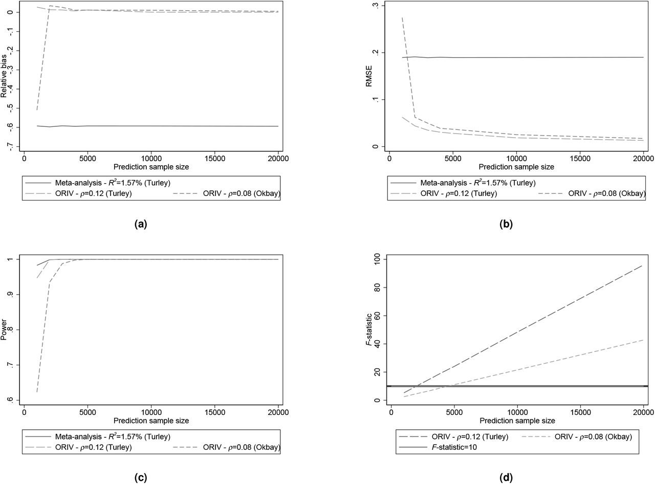
Relative bias, Root Mean Squared Error (RMSE), Statistical power, and first-stage F-statistic for meta-analysis (OLS) and ORIV for varying correlations between the ‘independent’ PGSs calibrated upon the phenotype well-being. The results are based on 1000 replications.
Together, these simulation results reiterate that the performance of meta-analysis versus (OR)IV is not driven by the absolute value of βst, but rather by the correlation between the independent PGSs (which in turn is driven by the explained SNP-based heritability) and the prediction sample size.
Polygenic scores
This study uses siblings in the UK Biobank (UKB) (60) as a holdout sample for constructing the polygenic scores (PGSs) and the empirical analyses. The GWAS discovery sample excludes these full siblings and their relatives up to the 3rd degree to ensure that the discovery and the holdout samples are independent from each other.
Relatedness
The UKB provides a kinship matrix, which contains the genetically identified degree of relatedness for pairs of UKB participants related up to a third degree or closer. The kinship coefficient is constructed using KING software (61). We use the following values of the kinship coefficient corresponding to each degree of relatedness: monozygotic twins (> 0.354), first degree parent-child or full siblings (0.177-0.354), and second and third degree relatives and cousins (0.044-0.177). In order to separate parent-child pairs from siblings, we use the identity-by-state (IBS0) coefficient, which measures genetic similarity in terms of the fraction of markers for which the related individuals do not share alleles (60). Given their kinship coefficient, parent-child pairs have IBS0 < 0.0012 and full siblings have IBS0 > 0.0012. After classifying all relationships, we separated those who are related to the siblings up to the third degree other than siblings themselves, i.e., parents of siblings and cousins of siblings (N = 14,947), and excluded those individuals from the GWAS discovery sample along with the full siblings. This ensures that our holdout sample of siblings is unrelated to the GWAS discovery sample.
Phenotypes
We follow the literature (see e.g. (11), (13), (31)) and convert an individuals’ highest self-reported educational qualification to equivalent years of education using the International Standard Classification of Education (ISCED). The resulting years of education phenotype ranges from 7 to 20, where College or University degree is equivalent to 20 years, National Vocational Qualification (NVQ), Higher National Diploma (HND), or Higher National Certificate (HNC) to 19 years, other professional qualifications to 15 years, having an A or AS levels or similar to 13 years, O levels, and (General) Certificate of Secondary Education ((G)CSE) to 10 years. If “none of the above” is selected, then the lowest level of 7 years is assigned. For height, we use the standing height (in centimeters) of participants measured as a part of the anthropometric data collection at the UKB assessment center. For both phenotypes, we impute the missing values in the first wave with the available information from the two follow up measurements in the UKB.
GWAS
We perform the GWAS on the UKB discovery sample for educational attainment (N = 389,419) and for height (N = 391,931), where both exclude siblings and their relatives (N = 56,450). For the split-sample PGSs, we first removed all remaining parent-child pairs (N = 5,084) and all cousins except one from each cousin cluster (N = 44,326). Thereafter, we split the unrelated discovery sample randomly into two parts of 170,004 for educational attainment and 170,937 for height. We use the fastGWA approach (35) as implemented in Genome-wide Complex Trait Analysis (GCTA), which applies mixed linear modeling (MLM) to genetic data and requires the following steps. First, based on the relatedness matrix, we generate a sparse genetic relatedness matrix (GRM). We then use the sparse GRM, the SNP data, and the respective phenotype file for height and educational attainment to run the GWAS. Each phenotype file contains a measure of the phenotype residualized with respect to month and year of birth, gender, interaction of birth year and gender, genotyping batch, and the first 40 principal components (PCs) of the genetic relationship matrix. Additional quality control includes cleaning the data with respect to exclusion of individuals who withdrew consent, with bad genotyping quality, with putative sex chromosome aneuploidy, whose second chromosome karyotypes are different from XX or XY, with outliers in heterozygosity, with missing gender or self-reported gender mismatching with the genetically identified gender, individuals of non-European ancestry, or with missing information on any of the former criteria, on the phenotype or on any of the control variables. Further, we perform quality control on the resulting GWAS summary statistics using the EasyQC tool (62).
Meta-Analysis
We meta-analyze our own GWAS summary statistics obtained with UKB data with the 23andMe summary statistics for the educational attainment PGS and with the GIANT 2014 summary statistics (20) for the height PGS using the software package METAL (63). While the GIANT summary statistics are publicly available, the 23andMe summary statistics are only available through 23andMe to qualified researchers under an agreement with 23andMe that protects the privacy of the 23andMe participants. For more information, visit https://research.23andme.com/collaborate/#dataset-access/. 23andMe participants were included in the analysis on the basis of consent status as checked at the time data analyses were initiated. Participants provided informed consent and participated in the research online, under a protocol approved by the external AAHRPP-accredited IRB, Ethical & Independent Review Services (EI Review).
Polygenic Scores
We construct the PGSs by accounting for the linkage disequilibrium (LD), i.e., the non-random correlations between SNPs at various loci of a single chromosome, using the LDpred tool (37), version 1.06, and Python, version 3.6.6. LDpred is a Python based package that corrects the GWAS weights for LD using a Bayesian approach. We follow steps as summarized by (10): (i) coordinate the base and the target files, (ii) compute the LD adjusted weights, and (iii) construct the polygenic score with PLINK (64) using the LD weighted GWAS summary statistics. The PGSs are based on approximately 1 million HapMap3 SNPs (we do not apply p-value thresholds). The final prediction (hold-out) sample consists of N = 35,282 siblings.
Acknowledgements
This research has been conducted using the UK Biobank Resource. The authors gratefully acknowledge participants of the 23andMe, Inc cohort for sharing GWAS summary statistics for educational attainment. The authors also acknowledge funding from NORFACE through the Dynamic of Inequality across the Life Course (DIAL) programme (462-16-100), from the European Research Council (DONNI 851725 and GEPSI 946647), from the National Institute on Aging of the National Institutes of Health (RF1055654 and R56AG058726), and from the Dutch Research Council (016.VIDI.185.044). We would like to thank Sjoerd van Alten, Ben Domingue, Michel Nivard, and Eric Slob for valuable comments. The contents of this article are solely the responsibility of the authors and do not necessarily represent the official views of the National Institutes of Health.
Footnotes
↵1 We follow (10) and define narrow-sense heritability,
, as the heritability estimate obtained in family-based (twin) studies, and SNP-based heritability, , as the proportion of phenotypic variance accounted for by SNPs on a standard genotyping chip. The GWAS-based heritability, , is the variance accounted for by genetic variants identified in a GWAS. That is, the R2 in a regression of the outcome of interest on the PGS. So .↵2 (10) and (14) define hidden heritability as the difference between
and . This part of heritability is ‘hidden’ because it will get smaller when GWAS discovery sample sizes increase.↵3 Based on a sample size of ~1.1 million, Lee et al. (11) construct a PGS explaining ~12%. This number is lower than theoretically predicted because of, amongst others reasons, the inclusion of samples from various countries in the GWAS meta-analysis.
↵4 The main assumption is that the two PGSs proxy for the same underlying ‘true’ PGS, and their sources of measurement error are independent. See the Methods section for more details about the assumptions.
↵5 To the best of our knowledge, only Kweon et al. (29) have previously applied IV in a within-family design.
↵6 The incremental R2 is defined as the absolute increase in R2 when the PGS is added in a regression, compared to a regression with only a standard set of control variables. For example, the incremental R2 of the PGS for EA in the latest large-scale GWAS of EA (EA3) is ~12% (11), and thus
. Then, if we assume that σPGS* = 1, the implied standard deviation of measurement error of this estimate is .↵7 These results were obtained using one randomly selected individual per family (N = 18, 989 for EA, N = 18, 913 for height). To obtain the LDSC estimate, the GWAS summary statistics were first computed using FastGWA (35). In the GREML analysis (36), the analysis sample was slightly lower (N = 17, 696 for EA, N = 17, 849 for height) because we excluded closely related individuals using the default relatedness cut-off of 0.025.
↵8 It is also lower than the reported R2 of around 12% in (11), but that study used a larger GWAS meta-analysis sample to construct the PGS and it also used different prediction samples.
↵9 Since environments differ, the best linear genetic predictor (i.e., the true latent PGS) may differ across samples. This would imply that the genetic correlation between the two samples would be lower than 1 for a particular outcome variable. This can be tested, for example with LDSC (7).
↵10 The correlation between the two polygenic scores is also an estimate of the ‘reliability’ of the polygenic score measure (39).
↵11 Note that the OLS and IV estimates are biased by a similar factor but in opposite directions. It follows that the square root of their product equals the true standardized effect
.


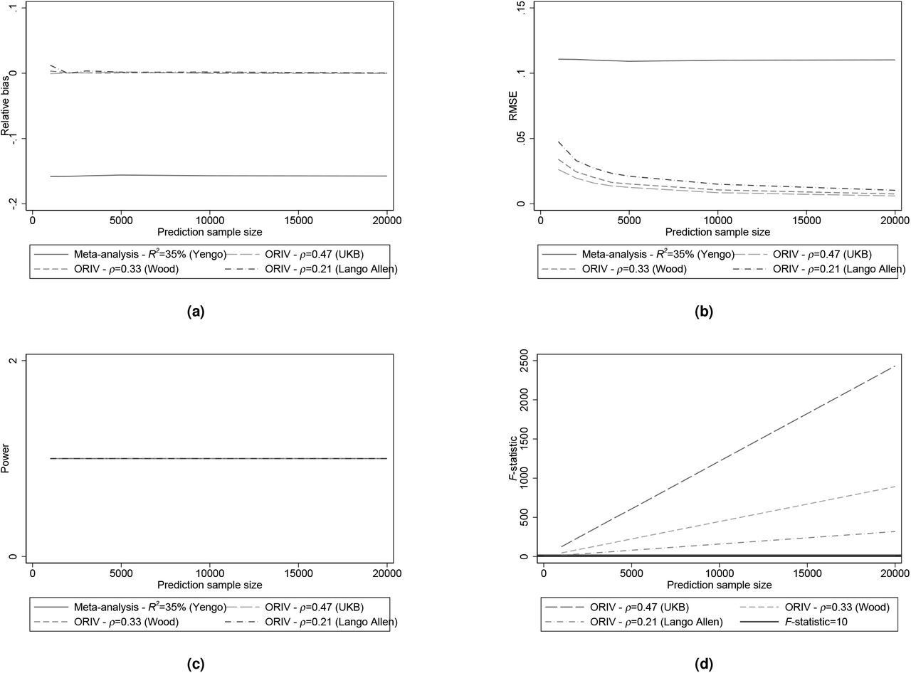
References


