

Summary
The spatial organization of the genome is essential for its functions, including gene expression, DNA replication and repair, as well as chromosome segregation1. Biomolecular condensation and loop extrusion have been proposed as the principal driving forces that underlie the formation of non-random chromatin structures such as topologically associating domains2, 3. However, whether the actual 3D-folding of DNA in single cells is consistent with these mechanisms has been difficult to address in situ. Here, we developed LoopTrace, a fluorescence imaging workflow for high-resolution reconstruction of 3D genome architecture that conserves chromatin structure at the nanoscale and can resolve the 3D-fold of chromosomal DNA with better than 5-kb precision in single human cells. Our results show that the chromatin fibre behaves as a random coil up to the megabase scale and is further structured by contacts between sites that anchor loops. Our single cell folds reveal that such looping interactions are sparse and lead to a large heterogeneity of folds with one or two dynamically positioned loop bases as the main reproducible feature of megabase scale chromosomal regions. Clustering folds by their 3D conformations revealed a series of structures consistent with progressive loop extrusion between major anchor sites. Consistently, the looping interactions and their non-random positioning depend on the presence of the loop extrusion enzyme cohesin and its anchor protein CTCF, respectively. Our approach is scalable and will be instrumental to image the functional 3D architecture of the genome directly at the nanoscale.
Main
The spatial organization of the eukaryotic genome covers a large hierarchy of scales, from the assembly of nucleosomes to supra-chromosomal compartments, and plays a central role in regulating genomic functions1, 4. Biochemical crosslinking and DNA sequencing-based chromosome conformation capture methods (3C/Hi-C) have revealed compartmentalization at the megabase (Mb) scale and topologically-associating domains (TADs) of several hundred kilobases (kb) as conserved features of chromatin organization3, 5. Boundaries of such TADs have been strongly linked to the position of CCCTC-binding factor (CTCF) binding sites3, 6 and the activity of the structural maintenance of chromosomes (SMC) family protein cohesin6–8, which has been shown to function as a molecular motor that can extrude DNA loops in vitro9. It has been proposed that in cells, chromatin-bound cohesin would promiscuously extrude loops in chromosomal DNA until encountering CTCF-binding sites10, 11. Computational models that combine loop extrusion activity with biophysical polymer models have indeed been able to simulate chromatin architectures consistent with Hi-C data12–15. However, direct evidence for the structure of individual loops and their formation by cohesin extrusion in single cells is lacking, largely due to technical challenges. Genome-wide maps of contact frequencies by Hi-C result from averages from large cell populations and do not contain single loop information16, while single-cell Hi-C methods provide only modest genomic resolution and sampling, precluding reliable detection of individual loops17, 18. In general, biochemical crosslinking and DNA sequencing-based methods do not directly report on the three-dimensional (3D) physical structure of chromatin in situ.
By contrast, microscopy-based methods such as fluorescence in situ hybridization (FISH) in principle offer direct, single-cell visualization of genome structure. The combination of the oligopaint technology, bar-coded labelling of many small genomic loci, and super-resolution microscopy techniques has indeed already enabled the visualization of genomic features with a genomic resolution down to several kb19–29. To explore the limits of the obtainable genomic resolution, we performed in vitro oligoDNA-PAINT on linearized single-stranded M13 bacteriophage DNA, showing that individual targets spaced only 64 bp apart can be readily resolved (Supp. Fig. S1a), which would be more than sufficient to trace loops predicted to be at least multiple 10s of kb in length30. In human cells however, efficient oligopaint labelling requires to open the genomic DNA double helix to ensure effective hybridization of only a small number of short FISH probes at each target locus. In most currently employed methods, cells are therefore treated with harsh DNA denaturation conditions, including hydrochloric acid and high temperature (80-95°C)23, 24, 26–28. Although this approach has successfully recapitulated the main features of HiC-based contact maps, significant perturbations of nuclear morphology and chromatin structure have been reported 21, 31–33, including the loss of structural details below 1 Mb as well as large scale DNA redistribution, such as loss of condensed chromatin regions, nuclear shrinkage and leakage of nuclear DNA into the cytoplasm33. Thus, standard FISH protocols currently used for chromatin tracing do not preserve that native architecture of chromatin at the nanoscale, which undermines the value of high-resolution structural information such as single chromatin loops that in principle could now be gained by oligopaint labelling and sub-diffraction imaging.

a, Overview of linearized single-stranded M13 bacteriophage DNA with biotin-associated docking handles (grey), 64-bp-spaced docking handles (P0, red) and ∼600 bp spaced docking handles (P1-P10) in orange to magenta colour scale used for 11-color-DNA-Exchange-PAINT, shown with an overlaid overview image overview and zoom-in of indicated regions. Scale 500 nm for image, and 50 nm for inserts. b, Schematic illustrating the alternative FISH approaches investigated in this work. c, FISH signal (peak intensity over background) with different total BrdU + BrdC concentrations (3:1 ratio) used for non-denaturing FISH. Data from n>50 cells per condition, representative of two independent experiments. d-g, Comparison of preservation of chromatin structure during individual steps of the FISH protocol: d, from live to fixed cells, e, from fixed to permeabilized cells and f, from permeabilization to acid treatment. g, Comparison of central and apical planes of cell nuclei (DNA stained with Hoechst) before and after FISH treatment using “tracing FISH” with acid treatment and 86°C denaturation, “3D FISH” with acid and 75°C denaturation and non-denaturing FISH. Scale bars, 5µm; RDs in f, 1 µm. Images representative of >10 (a) or >50 cells (d-g) in two independent experiments.
In order to investigate the nanoscale folding of single chromatin fibres in situ, we therefore developed a high-resolution chromatin tracing workflow extending previous work on non-denaturing FISH after strand-specific enzymatic digestion of DNA (CO-FISH/RASER-FISH)34–37 and combining it with sequential labelling by state-of-the-art oligopaint FISH probes. Using this approach, which we term “LoopTrace”, we systematically investigate the 3D-folding of chromatin in several genomic regions from the few kb to Mb-scale in single human cells. We demonstrate that our approach offers superior preservation of nuclear and chromatin structure and yet enables effective probe hybridization and thus very high-resolution 3D chromatin tracing at the scale of single loops. Our 3D traces from many hundreds of single cells show that in the absence of structuring elements such as CTCF binding sites, the 3D-fold of the chromatin fibre is fully consistent with a random coil. Mining our data for structural similarity between single-cell-folds using non-supervised and supervised clustering revealed that genomic regions containing multiple CTCF-binding sites display cohesin- and CTCF-dependent sparse looping interactions. Their size and frequency is fully consistent with dynamic loop extrusion, and their cumulative effect explains the emergence of TAD-like features at the population level.
Non-denaturing FISH preserves nuclear structure
To investigate which FISH protocol would best preserve chromatin structure while meeting the demanding labelling efficiency requirements of high-resolution chromatin tracing, we compared three protocols: High temperature denaturing FISH (“tracing FISH”) 23, 24, 26–28, a slightly lower temperature denaturing FISH (similar to “3D-FISH”), which has been reported to improve chromatin structural preservation21, and a non-denaturing FISH approach (CO-FISH or RASER-FISH, see schematic in Supp. Fig S1b)34–38, which relies on enzymatic strand resection to render long stretches of DNA single stranded, and uses no heat or acid treatment. To compare the methods, we first labelled a 10 kb single-copy region in the MYC locus of human diploid RPE-1 cells with 96 oligopaint probes (Fig 1a). “Tracing-FISH” showed chromatin leakage into the cytoplasm33 and more than the two expected FISH signals, also in regions extruded from the nucleus. 3D-FISH and non-denaturing FISH showed no such large scale artefacts but had slightly (non-denaturing, after protocol optimization, see Supp. Fig. S1) or significantly (3D-FISH) lower labelling efficiency than “tracing FISH” (Fig. 1b).

a, Diploid RPE-1 cells were prepared with alternative FISH protocols and labelled with 96 primary oligonucleotide FISH probes targeting a single copy 10 kb region upstream of the MYC gene on chromosome 8, visualized with an Atto565-labelled imaging oligo. FISH signal in extra-nuclear DNA material is indicated with the arrow. Maximum z-projections are shown. b, Peak signal intensity over background of FISH spots fit with a 3D Gaussian function for alternative FISH protocols. Data from n>50 cells per condition, representative of 2 independent experiments. c, Structural preservation of nuclear architecture after alternative FISH protocols, assessed by structured illumination microscopy (SIM) of cells labelled with Hoechst (DNA, grey) and Atto647-dUTP (replication domains, RDs, magenta/green). Extra-nuclear DNA material and substantial shifts in RD position indicated by arrows. Single z-planes are shown. d, Pearson’s correlation of signal intensity of 3D drift-corrected SIM images before and after FISH. Data from n>350 cells per condition from two independent experiments. e-f, Comparison of a sequential FISH imaging targeting ten 5 kb regions tiled across 100 kb in the MYC locus using e, high-temperature denaturing FISH and f, non-denaturing FISH. Single z-slices are shown. Data representative of e, 431 cells in one experiment or f, 562 cell in 3 experiments. Scale bars: a and c, 5 µm (FISH/DNA), and 1 µm (RDs/DNA zoom), e and f, 500 nm.
To investigate chromatin structure preservation in more detail, we imaged cell nuclei at each major step in the FISH protocols using structured illumination microscopy (SIM) 21. We visualized general genome structure with the DNA-binding dye Hoechst as well as the TAD-level structure of co-replicating domains using co-replicatively incorporated fluorescent dUTPs39. While the initial fixation and permeabilization steps did not substantially alter genome or TAD level structure (Supp. Fig. S1d,e), the standard denaturation steps with hydrochloric acid and/or denaturation at 86°C24, 27–29 led to significant structural changes (Fig. 1c,d, Supp. Fig. S1f,g), including fragmentation of heterochromatin, loss of nuclear integrity, spilling of DNA into the cytoplasm, and displacement/loss of co-replicating domains. 3D-FISH showed milder but still significant perturbations of genome architecture, while non-denaturing FISH showed best preservation of overall genome as well as TAD level architecture.
To validate the FISH protocols for 3D reconstruction of genome folds, we carried out preliminary tracing experiments using ten 5 kb probe-sets tiled along a 100 kb region upstream of MYC. Here, high temperature denaturing FISH frequently showed multiple lower signal intensities spread out over larger regions suggesting chromatin fragmentation, which is incompatible with high precision chromatin tracing (Fig. 1e). By contrast, non-denaturing FISH showed highly consistent labelling of diffraction-limited regions (Fig. 1f), which is the expected native behaviour from orthogonal labelling methods39, 40. In summary, non-denaturing FISH combines good hybridization efficiency of oligopaint probes to genomic DNA with near-native preservation of nuclear structure, which makes it a suitable method to investigate the folding of chromosomal DNA at the nanoscale in situ in single human cells.
High-throughput 3D-chromatin tracing at single-loop-scale
Having a structure preserving probe-binding protocol at hand, we next developed a robust sequential DNA-FISH imaging workflow (LoopTrace) to achieve high-resolution 3D-chromatin tracing at the scale of single DNA loops. To establish a baseline, we first aimed to reconstruct unconstrained, open euchromatin, and therefore chose a non-coding genomic region upstream of the MYC gene on the right arm of chromosome 8 (Fig. 2a), predicted to have little conserved structure (Supp. Fig. 2a) and containing no CTCF-binding site (Fig. 2a). We targeted ten discrete 5-kb-loci spaced 5 kb apart with a set of oligopaint probes containing locus-specific barcodes. The primary probes were detected by sequentially hybridizing and imaging ten different fluorescent 12-bp imager strands matching each locus barcode41. The fully automated workflow (see methods and schematic in Supp. Fig. S2b), with rapid hybridization and washing cycles allowed us to reach a throughput of about 1000 cells/day.
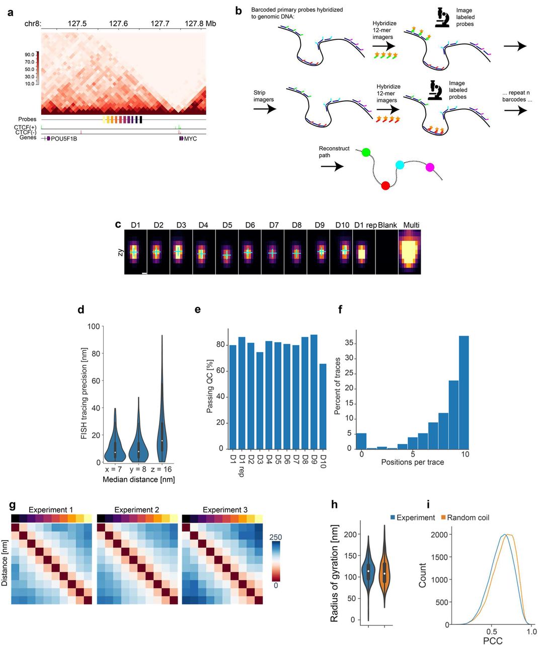
a, Hi-C contact map of RPE-1 cells (GSE71831) at 10 kb binning of the traced region in the vicinity of the MYC gene, with probe positions, CTCF chip-seq peaks indicated by direction of the predicted overlapping binding motif (see methods), and genes (GENCODE). b, Schematic of chromatin tracing strategy used in this work. c, Slices along the zy axis at the central x position with fit positions overlaid for an exemplary D1-10 sequential hybridization, corresponding to main Fig. 2b. d, Tracing precision in x, y and z estimated by relabelling the first position (D1) after completing D1-10 hybridizations, with median distances as indicated. Data from n=161 traces from one representative experiment. e, The percentage of hybridizations detected and passing quality control (QC) in all traces. f, Percentage of traces with indicated number of hybridizations detected and passing QC. Data in e and f from 223 traces in one representative experiment. g, Distance maps for replicate experiments tracing the same region as in Figure 2. Experimental replicates show highly similar distance matrices with average Pearson’s correlation of 0.97. n=138, 203 and 182 traces for experiments 1, 2, and 3, respectively. Scale bar in nm. h, Distribution of the radius of gyration of experimental traces and traces from the random coil model. No difference was detected (two-sided Mann-Whitney test, p=0.11). n=220 traces per sample. Only full-length traces were included from the experiments to ensure that the radii of gyration are comparable. i, Kernel density estimates of all pairwise Pearson’ correlation values of traces aligned by 3D rigid registration in the experimental dataset and an equal number of random coil models.

a, Overview of a non-coding region upstream of MYC gene selected for tracing pipeline validation with genes and CTCF sites (RPE Chip-seq) highlighted. The probes cover 10 regions of 5 kb with 5-kb-gaps, spanning a total of 100 kb. b, Exemplary field of view and selection of one tracing region by FISH signal (orange) in a single nucleus (Hoechst, blue), an overlay of probe signals (maximum projection in z) after drift correction and centroid fitting of FISH spots (multi-coloured crosses indicate fit positions). Scale bars, 20 µm, 5 µm and 200 nm. c, 2D projections of fit FISH signal coordinates in xy or zy direction. Scale bars, 100 nm. d, Individual FISH signals at the central z-plane of each fit from sequential hybridization of the 10 labelled regions (D1-D10), as well as repeat labelling (D1 rep), wash buffer only (Blank) or simultaneous labelling with multiple probes for region identification (Multi). Fit centroid positions are indicated by blue crosses. Scale bar, 200 nm. e, Example of 1D-signal (black) from a FISH spot, and a 1D-Gaussian fit (red line) to the signal that is used for centroid fitting. f, Tracing precision judged by 3D-Euclidean distance across 10 hybridizations, measured on fiducial beads (n=66, median=14 nm) or by re-hybridizing the first position after tracing (n=161 traces, median=24 nm). Data from one representative of 8 experiments. g, Examples of FISH signal, centroid fitting projection and resulting 2D-projected (see methods) chromatin traces from 6 different cells. Scale bars, 5 µm (cells), 200 nm (insets) and 100 nm (traces). h, 2D-projected consensus traces of D1-10 probe positions generated by general Procrustes analysis, overlaid with kernel density estimates (KDE) of aligned single trace data (see methods), and median pairwise distance map for probe positions D1-10. Data from n=469 and n=523 traces (filtered for at least 70% or 50% completeness, respectively, see methods for details) from 3 experiments. i, Equivalent representations of a random coil model with 10 equally spaced positions scaled by the experimentally determined parameters (see methods). Data from n = 469 and n = 523 simulated traces. Scale bars, h, i: 100 nm, colour map scale is in nm. j, The difference between the experimental and random coil distance matrixes after z-score normalization of the data, highlighting distances which are smaller (orange) or larger (purple) than expected compared to the model. k, Scaling relation between the spatial distance measured between all pairs of probes and the genomic distance of probe hybridization targets. The data was fit to a square root dependence (orange dashed line). Data from n=523 traces in 3 experiments.
We found that our workflow produced reproducible FISH signal which was completely removed in the washing step, enabling reliable reconstruction of chromatin paths (Fig. 2b-d, Supp. Fig. S2c). To estimate the tracing precision we could achieve, we re-localized the first locus after ten rounds of hybridization, having continuously drift-corrected the data using fluorescent beads in a separate channel (Fig. 2e, f). The bead-based drift-correction had a median 3D-distance error of <15 nm as determined by 3D-Gaussian fitting. Re-localization of the first locus showed a median 3D-distance deviation of <25 nm (Fig. 2f), or 7, 8 and 16-nm deviations along x, y and z, respectively (Supp. Fig. S2d), demonstrating that our approach is suitable for high-precision 3D-chromatin tracing well below the diffraction limit. LoopTrace was also highly efficient, as at least 90% of sequential hybridizations were detected in the majority of cells imaged (Supp. Fig. S2e, f).
A loop-scale region upstream of the MYC promoter behaves like a random coil
Comparing the 3D-traces of the 100-kb-region upstream of the MYC promoter in individual cells showed substantial cell-to-cell variability of chromatin structure (Fig. 2g). Combining the data from hundreds of cells into consensus chromatin traces by general Procrustes analysis (see methods) or pairwise median distance maps of all loci reproducibly showed no clear substructure (Fig. 2h; Supp. Fig. S2g, average Pearson’s correlation coefficient r = 0.99 between replicate median distance matrices).
As a polymer, the chromatin fibre is predicted to fold like a random coil in the absence of structuring elements or other binding interactions. We therefore compared our experimental data of this region with the 3D-fold calculated from a random coil model of chromatin with an equidistant step size of 90 nm, matching the median physical distance of our FISH loci (Fig. 2i). Comparing the consensus traces or pairwise distance maps between experiment and model showed almost perfect agreement (Fig. 2h,i, r = 0.98) and only little residual deviation could be detected by a z-score normalized difference, or by comparing radii of gyration or the pairwise similarity of 3D-aligned traces with the random coils (Fig. 2j, Supp. Fig. S2h,i). Interestingly, our experimental data allowed us to determine the relationship between genomic and physical distance for this unstructured region of euchromatin. Again, as expected for a random coil, we found that the spatial distance scaled with the square root of the genomic distance in this region with a scaling parameter of 24.7 nm/kb2 (r2 = 0.94), a valuable parameter to constrain theoretical models of chromatin folding.
The TAD-scale regulatory region upstream of the MYC gene shows non-random structure
Given that our method could capture the highly variable and therefore likely dynamic structures of a relatively short stretch of euchromatin, we tested next if it can also resolve the boundaries of compact domains and individual loops predicted by biochemical approaches. To this end, we probed a larger, TAD-scale euchromatic region spanning the entire regulatory domain upstream of the MYC gene with ten probes situated at 50-200 kb intervals across this 1-Mb-region (Fig. 3a, Supp. Fig. S3a). This region is predicted to contain a number of frequently occupied CTCF binding sites and we targeted the four most prominent of them directly with our probes (Fig. 3a, probes H2, H4, H6, H9).

a, HiC contact map of RPE-1 cells (GSE71831) at 10 kb binning of the TAD-scale region in vicinity of the MYC gene selected for chromatin tracing, with probe positions as indicated, and the ∼100 kb region traced previously indicated in blue. b, Median pairwise distance map and pairwise contact frequencies (defined as <150 nm 3D distance) of detected probe coordinates. n=775 traces from 3 experiments. Pearson’s r values for the distance (rd) and contact maps (rc) as indicated were calculated vs. the random coil model. The rd value of 0.78 is significantly lower than the corresponding value for the loop-scale region (Fig. 2) of 0.98 (Fisher’s z-transformation test, p<0.01), indicating a less random structure. c, Median distance map and contact frequencies of random coil model scaled according to the experimental data derived earlier (see main Figure 2 and methods for details), and z-score normalized difference between the experimental and random coil distance maps. n = 775 traces were simulated. Scale bars in b and c in nm. d, Consensus traces and pairwise contact frequencies of all clusters identified by non-supervised clustering in main Fig. 3e. e, Exemplary single traces and contact maps from cluster 1 (blue) or cluster 9 (green). The contact maps highlight (white features) positions with a 3D pairwise distance less than 150 nm. f, Quantification of the number of contacts per cell in the experimental data compared to a random coil. n=613 experimental traces after filtering for >=80% completeness. An equal number of random coils were simulated with identical position drop-out rates for comparison to the experimental data. Differences were assessed using a two-tailed Mann-Whitney U test resulting in the indicated p-value. g, Consensus traces and pairwise contact frequencies of clusters filtered for proximity between H2 and downstream positions (H3-H9). h, Distributions of pairwise distances between the indicated positions in the full experimental dataset (n = 775 traces) or only those that contained the H2-H9 loop (pairwise distance below 150 nm). The boxplots indicate quartile values and the median, the whiskers show data range excluding outliers. Data are colour-coded by traces with the indicated positions having 3D pairwise distances above (blue) or below (green) 150 nm, the frequencies are indicated below each graph. Differences were assessed using a two-tailed Mann-Whitney U test resulting in the indicated p-values.

a, Overview of the genomic region investigated, spanning 1.1 Mb in a regulatory region upstream of the MYC gene in chr8. 10 barcoded ∼3-5 kb-sized probe sets were designed for this region targeting loci of interest such as several CTCF sites and the MYC promoter and gene. b, Image of a representative RPE-1 cell trace. The tracing region with a FISH signal (orange) is highlighted in the nucleus (blue) and single hybridizations and their centroid fits (coloured crosses) are shown with a multi-colour overlay of the sequential FISH spot images. Scale bars, 5 µm (left) and 200 nm (right). c, 2D-projection in the xy-plane of the chromatin trace resulting from the fits in b. d, Best-fit 2D projections of the consensus trace of the experimental data and the corresponding random coil model, overlaid with kernel density estimates of the aligned individual traces. Data from n=775 traces in 3 experiments, or 775 simulated traces. e, Result of trace clustering by UMAP dimensionality reduction followed by variational Bayesian estimation of a Gaussian mixture, based on similarity between pairwise distances of each chromatin trace. The consensus traces for selected clusters are shown in matching colours. n = 40-100 traces per cluster. f, Consensus traces filtered for a 3D pairwise distance of less than 150 nm between positions H2 and H3, H4, H6 and H9. The position of the proximal interaction between H2 and H3-H9 are indicated with a blue ring of 150 nm in diameter. n = 50-100 traces per cluster. Scale bars in c-f are 100 nm.
Sequential imager strand exchange and high-precision imaging of the ten loci (H1-10) resulted in 3D-localization data of very similar quality as for the shorter unstructured region (Fig. 3b, c), with an overall median 3D-tracing precision of ∼25 nm. 3D-traces from single cells showed clear indications of loop-like features (Fig. 3b, c). Integrating the 3D traces from ∼800 cells into consensus traces, median pairwise distance maps or contact frequency maps (Fig 3d, Supp. Fig. S3b) further confirmed the presence of looping conformations distinct from the random coil model (Fig. 3d, Supp. Fig. 3c), and could clearly identify the TAD boundaries at probes H2 and H9, consistent with data from population Hi-C experiments, validating our high-precision 3D-imaging approach (Supp. Fig. S3b). In contrast to the smaller non-structured region, the median distance matrix of the TAD-scale region thus deviated significantly from the predictions of the random coil model with high residual z-score differences, and a strong enrichment of long range interactions between H2 and several downstream loci (Supp. Fig. S3b-c, Pearson’s r=0.78). This significant non-randomness of our experimental traces suggests the presence of interactions that stabilize long-range contacts, such as cohesin complexes.
Unsupervised and supervised clustering reveal structural intermediates consistent with progressive loop extrusion
Interestingly, most pairwise contacts were only present in 5 – 15 % of cells (Fig. S3b) and we therefore hypothesized that they may represent different states of a dynamically changing structure, which would be only poorly represented in the overall average of all traces. To test this, we performed unsupervised clustering of the individual traces based on their pairwise similarity, putting a stronger weight on the shorter pairwise distances that might indicate contacts (Fig. 3e and Supp. Fig S3d, see methods for details). Indeed, each cluster had different structural features in its consensus trace. While the broader clusters (e.g. clusters 1-3) were similar to the overall average in containing multiple low-frequency contacts, the tighter clusters (e.g. clusters 8-10) were highly enriched in only 1-2 specific long-range contacts and showed clear loop-like features. Inspection of single cell traces (Supp. Fig. S3e) confirmed that although single cells vary strongly in overall conformation, contacts (<150 nm) at the base of loop-like conformations are present in most cells. Comparing single traces from the broad cluster 1 with the tight cluster 9, showed that contacts are more consistently positioned in the tighter cluster. Finally, quantifying the number of contacts per trace across all traces of this region showed that contacts are significantly enriched compared to the random coil model, but remain sparse with individual chromatin fibres displaying a median of 3 out of the 45 possible pairwise contacts (Supp. Fig. S3f).
Our unsupervised clustering showed that the same TAD scale chromatin region can be in different structural states that exhibit contacts at the base of loop-like conformations in different positions along the fibre. This behaviour is expected for a random coil with the additional constraint of interactions that would stabilize long range contacts. While cohesin has been shown to be able to interlink distant positions along a chromatin fibre6,7, the current hypothesis is that they function by active loop extrusion1, 11, rather than randomly connecting two loci. To test if our data would be consistent with processive loop extrusion operating in cells, we performed supervised clustering by selecting single cell traces with pairwise contacts (< 150 nm) between H2 and probes further downstream in this TAD scale region (Fig. 3f, Supp. Fig. S3g). H2 was chosen as it was the upstream anchor in the dominating pairwise contacts in 5 out of 9 unsupervised clusters (Supp. Fig. 3d), consistent with it overlapping with a major CTCF site. This supervised clustering by contacts in genomic proximity to H2 was indeed consistent with intermediates of a progressively extruded loop, where H2 contacts further and further downstream loci and extrudes a loop of increasing size. Interestingly, while most of these contacts were relatively rare, with a frequency of ∼8-10% of all cells, those connecting H2 to the other two major CTCF sites H4 and H9, which are convergent to H2 (Supp. Fig. S3a, g), appeared to be stabilized with a frequency of 15-17%. Overall, our data is therefore fully consistent with a progressive loop extrusion from H2 towards H9 across a genomic distance of ∼800 kb.
TAD features only emerge in population averages of single loop conformations
We choose the upstream regulatory region of the MYC gene because of its clear TAD signature in HiC data (Supp. Fig. S3a). However, none of our single cell traces or unsupervised clusters, if converted into contact frequency maps, matched the HiC TAD (Supp. Fig. S3d,e). To better understand how our single cell 3D traces lead to the features of TADs, we investigated the overall structural effects of the largest loop (H2-H9) on the whole region in more detail (Supp. Fig. S3f) by comparing cells containing the H2-H9 loop with the entire population. In the presence of this loop, the pairwise distance between H1 (outside the TAD) and H2 (TAD boundary/loop base) is strongly increased, while pairwise distances remain similar between positions outside and inside the loop (e.g. H1 v. H3 or H5), or between two loci inside the loop (e.g. H7-H8 and H5-H8). Thus, the presence of the H2-H9 loop mainly alters the structure by bringing the loop anchors into close proximity and apparently pulling them away from immediate neighbouring genomic positions, but do not otherwise alter interactions occurring further inside or outside the loop. Consistently, if one excludes the H2-H9 interaction, the overall contact frequencies are highly similar between the cells containing the H2-H9 loop compared to the entire population (Supp. Fig. S3b, e). Combined with our data showing that the 100 kb region situated between the H8 and H9 probes behaves as a random coil, we conclude that most likely the entire 1.1 Mb TAD-scale regulatory region of the MYC gene effectively behaves as a random coil constrained by a few non-random long-range looping interactions. We could thus directly observe from single cell 3D folding data how the cumulative effect of sparse looping interactions gives rise to the impression of internally more highly interacting TADs and TAD boundaries in population averages. It is interesting to note that neither a clear TAD boundary, nor an overall higher probability of interaction inside the TAD is observed at any given time point represented by the large number of 3D snapshots from single cells.
TAD-scale genomic regions on different chromosomes exhibit non-random looping conformations including stacked loops
If the cumulative effect of dynamically positioned 3D looping conformations of the chromosomal DNA explain TAD-like features, we should find them on different chromosomes, in eu- and heterochromatin (or active and inactive compartments) and different cell types, where TADs have been observed by HiC. To more broadly investigate TAD-scale looping interactions beyond the MYC locus of RPE-1 cells, we therefore next traced four additional 1.3 to 1.8 Mb sized regions with typical TAD features (Supp. Fig. S4a) in HeLa cells. The targeted regions included two transcriptionally active regions on chromosome 2 and 742 (chr2-A, chr7-HoxA; A compartment), one region transcriptionally inactive region on chromosome 4 (chr4-B; B compartment), and one region with mixed activity on chromosome 7, more similar to the MYC locus (chr7-SHH; mixed compartment) (Supp. Fig S4a). Consistent with the findings from the MYC locus, our 3D chromatin tracing consistently identified sparse, non-random looping interactions in single cells giving rise to emergent TAD-like structures cumulatively, consistent with the available HiC data (Fig. 4a-c, Supp. Fig. S4b). The number of contacts per chromosomal region was similar with a median of 3 contacts across the 10-12 probes targeting CTCF sites and intermediate loci. Using the chr7-SHH region as an example, unsupervised clustering of single cell traces identified classes of 3D folds with similar overall features as in the MYC locus (Supp. Fig. S4c), including broader clusters with less reproducible folds, and tighter clusters enriched in specific contacts highlighting looping interactions. Interestingly the arrangement of CTCF sites in the chr7-SHH region is such, that the dominant CTCF site at the TAD boundary targeted by the H3 probe could form two different loops, to the convergent CTCF sites targeted by the H7 and/or the H9 probes. This provided the opportunity to ask if stacked loops, which have been debated in the literature1, 13, 43 can actually be observed in single cells, i.e. if the H3-H9 loop could coincide with H3-H7. Indeed, of the 18% (n=308 out of 1725) of the cells that contained the H3-H9 contact, 43% (n=118 out of 275) also contained the H3-H7 contact, showing that stacked loops occur rather commonly in single cells (Supp. Fig. S4d, e).

a, HeLa HiC maps (GSE63525) binned at 10 kb of the 4 additional regions selected for tracing. The probes, as well as HeLa CTCF CHIP-seq peaks encoded for motif directionality, HeLa Rad21 CHIP-seq peaks and SNIPER compartmental annotations are also included. b, Median pairwise distance maps and pairwise contact frequencies (defined at 150 nm 3D distance) of detected probe coordinates in the 4 indicated regions in HeLa cells. n numbers as indicated from 3 experiments. c, Clustering example of single traces from the chr7-SHH locus in wild type HeLa cells (left), with consensus traces (middle) and contact frequencies (right) of exemplary clusters indicated by trace/cluster colour. n=1759 from 3 experiments, each cluster n=40-300 traces. d, Three-way interactions in the SHH locus, exemplified by the long-range H3-H9 contact co-occurring with the shorter range H3-H7 and H7-H9 contacts, indicating three-way contacts occurring in a subset of the cells showing the H3-H9 contact. The frequency of cells where the contact occurs are indicated and corresponding number of traces in each group are indicated, in the right panel the percentage indicates the occurrence of the H3-H7 contact in cells with the H3-H9 contact. e, Exemplary single cell traces and contact maps from the group containing the double H3-H7 and H3-H9 contacts identified in d. f, Chemiluminescence signal from simple Western assay using anti-Rad21 in HeLa Rad21-GFP-AID cells untreated or treated with auxin (IAA), auxinole or both for the indicated durations. Yellow and cyan markers indicate technical duplicates from one experiment. g, Pearson’s correlation coefficients (r) of the pairwise distance and pairwise contact maps between the indicated experimental conditions and the matching random coil model. n number per condition as indicated in Fig. 4b. Scale bar in c-e, 100 nm, f, 50 µm.

a, Overview of barcoding strategy to simultaneously acquire data from multiple cell-lines. Each of up to four cell lines is either left unlabelled, or pre-labelled with VF405, VF488 or both before mixing and seeding the cells in the sample chamber. After fixation, VF405 and VF488 signals in cells in the entire sample chamber are imaged at lower magnification, then labelled with DAPI and reimaged before being processed for FISH. The same cells are relocated by registering the DAPI channel acquired during sequential FISH imaging with the pre-FISH images, and detecting the VF405 and VF488 intensities in a dilated nuclear mask (pseudo-coloured ellipses). The original cell types are then recovered by a manual gating strategy based on the VF405+VF488 intensity. Imaging representative of 100 fields of view in 2 experiments. b, All pairwise intra-cluster differences (using √ 1 − PCC) as distance metric) of traces from the MYC locus TAD-scale region assigned to clusters in main Fig. 3e (left), compared with randomly permuted cluster memberships (right). Overall differences detected by comparing the means of the real and permuted clusters (p=1e-5, two-tailed t-test, total of n=775 traces in 10 clusters). Results were identical for repeated permutations.

a, Overview of the 4 genomic regions investigated in HeLa cells with 11 probes across 1.6 Mb (chr2:171.3-172.9 Mb, A-compartment), 10 probes across 1.3 Mb (chr4:12.5-13.8 Mb, B-compartment), 11 probes across 1.8 Mb (chr7:25.6-27.4 Mb, mixed compartment, HoxA locus) and 12 probes across 1.6 Mb (chr7:155.6-157.2 Mb, mixed compartment, SHH locus). Each probe targeted a ∼10 kb-sized region. b, Consensus traces and contact frequencies of wild type HeLa Kyoto cells or HeLa Kyoto cell lines with Rad21 (cohesin), CTCF or WAPL endogenously tagged with AID. Cells were acutely depleted of the respective proteins by 2 h auxin treatment. Traces filtered for >=67% completeness. Data from 3 (wild type) or 2 (AID-lines) experiments, number of traces per condition as indicated. Random coil models generated for each region are shown for comparison. c, Single trace examples and contact maps (<150 nm) from wild type cells and cells depleted of the indicated proteins. Scale bars 100 nm. d, The number of contacts per trace for the different regions and perturbations indicated and compared to the random coil model. † p<0.05 for condition vs. random coil, * p<0.05 for condition vs wild type, tested by Kruskal-Wallis non-parametric 1-way ANOVA followed by Conover’s test with step-down Bonferroni adjustment for multiple comparisons. Traces filtered for >=80% completeness, and an equal number of random coils were simulated with identical position drop-out rates for comparison to the experimental data. Total of n = 7983 single experimental traces from 7 experiments.
Looping interactions depend on cohesin and CTCF in single cells
Our data so far is consistent with a model that chromosome regions up to the megabase scale behave like a random coil that is structured by long-range contacts which result from dynamic, progressive loop extrusion, with loop base contacts becoming stabilized at strongly occupied, convergent CTCF sites. This model would predict that looping conformations should depend on the loop extrusion enzyme cohesin and its regulators. To test this, we decided to acutely remove cohesin, CTCF6, 7 and the cohesin unloader WAPL44, 45 from HeLa cells where these genes had been homozygously engineered with the AID degron tag6. After short-term treatment with the degradation inducing hormone Auxin, the proteins were efficiently depleted (Supp. Fig. S4f and 6), and we could study their requirement for chromatin folding at the single cell level by 3D single cell tracing of the same four genomic regions in HeLa cells.
Strikingly, cohesin (Rad21) depletion reduced pairwise contacts to levels of random coils for all four regions. Their consensus traces thus showed open, mostly contact-less folds, which was confirmed by inspecting single cell 3D folds (Fig. 4a-c, Supp. Fig. 4g). Consistently, the corresponding contact frequency maps of all 3D traces showed dramatically reducing internal contacts and disappearance of TAD boundaries. By contrast, removal of the cohesin unloader WAPL led to increased compaction of the regions and a clear increase in the number of contacts from a median of 3 to 4 per chromosomal region (Fig. 4c), and in reproducibly positioned loops, such that the non-random structure become further enhanced in the overall consensus traces and single cells compared to wildtype (Fig. 4a,b, Supp. Fig. S4g). WAPL depletion furthermore led to an accumulation of longer range contacts, partly at the cost of shorter-range contacts (Fig. 4a), consistent with previous findings 6, 46. Inspecting the single cell traces (Fig. 4c) shows that although looping significantly increases, loops remain relatively sparse, suggesting that even an increased amount of cohesin mainly causes a few point-like contacts in single cells rather than leading to a complete collapse of entire TAD-scale regions into an inaccessible compact domain.
CTCF removal should not affect the amount of cohesin on chromosomes but rather affect its positioning to CTCF sites. Consistent with this, CTCF depletion led to a loss of specifically positioned contacts in consensus traces and single cell folds (Fig. 4a, b). In contrast to cohesin degradation that abolished most contacts, the number of contacts in single CTCF-depleted cells remained similar to wild type (Fig. 4c) but their positions were no longer reproducible, fully consistent with CTCF’s role in anchoring cohesin47 but not being required for its activity per se. Nevertheless, the more randomly distributed contacts formed without CTCF still led to an overall compaction of the regions, that now resembled a compacted random coil, devoid of reproducibly positioned looping features (Fig. 4b). Taken together, our acute removal of cohesin, its removal factor or its anchor demonstrate that cohesin activity and anchoring is required for the formation of reproducible looping conformations in the 3D chromatin fold of single cells. These findings are fully consistent with the variable yet reproducibly positioned looping architectures we observe in snapshots of hundreds of single cells to result from progressive loop extrusion of an average of only 1 to 2 loops per megabase scale chromosomal region.
Discussion
The “LoopTrace” workflow we introduce here provides a powerful approach to investigate the nanoscale folding principles of chromatin in situ in single cells. By using an enzymatic non-denaturing FISH method, we could gain superior preservation of native chromatin structure and yet achieve a sufficiently robust FISH signal from small sets of oligopaint probes to allow reliable 3D-chromatin tracing of loop-scale features with high genomic resolution and spatial precision. While our method does not suffer from the micron scale structure artefacts of denaturation-based FISH methods, we note that even the non-denaturing FISH approach shows milder alterations of nuclear structure, such as slight swelling of nucleoli and moderate changes in nuclear shape. In the future, hopefully even more native methods of making genomic DNA accessible for efficient binding of sequence specific probes can be developed. Our throughput currently reaches 1000 traced cells/day by using short 12-bp imagers for fast exchanges, and the combined use of cell and probe barcoding strategies. These multiplexing features can be substantially extended in the future, allowing scaling of the method to more and larger genomic regions, as well as integrating multi-scale sampling strategy, allowing to combine information from high resolution tracing with genomically sparser, but still high precision, sampling to span multiple genomic scales and structural features.
Our data provides an informative, directly spatially measured, dimension to the understanding of the folding principles of the genome in situ. Based on indirect HiC data and computer simulations, cohesin driven loop extrusion had been hypothesized to potentially be the mechanism through which this SMC protein and its regulators drive TAD formation6, 7. However, a direct visualization of the proposed looping conformations of genomic DNA has so far been lacking. Our 3D tracing data in single cells for the first time provides such direct evidence and shows that an unstructured region of chromatin indeed folds like a non-interacting random coil onto which consistent loops are superimposing when it contains CTCF sites. We find that these loops are generally sparse, on the order of 1-2 per megabase region, and highly dynamic with intermediate states of increasing loop size, consistent with progressive loop extrusion.
This dynamic nature means that even the most stably anchored position of a loop we have observed was only present in 15-40% of the cells in a population. This is however sufficient to give rise to substantial non-random interactions that strongly influence the overall structure of the region, most prominently directly adjacent to the loop base. A single, isolated loop pulls its anchors together, physically removing them from directly neighbouring regions, indicating a lack of mechanical coupling at this scale (∼100 kb) at least for as long as it takes for cohesin to generate a loop, most likely a time scale of several minutes9, 48. This is consistent with observations in live cells that reported rapid loss of mechanical coupling along the chromosomal fibre over only a few 100s of nm39. Interestingly, besides the strong effect directly at the loop base, large loops neither effect the frequency nor position of interactions of loci inside the loop, nor their interactions with loci outside loops, suggesting that the chromatin fibre is highly flexible and operates like a random coil again at distances above ∼100 kb from the loop base. The complete set of TAD features, i.e. strong boundaries and high frequency of internal loop interactions thus does not exist in any single cell at any time point. Rather, TAD boundaries in cell population data arise from the cumulative effect of dynamically positioned sparse looping interactions inside the TAD.
Our removal of cohesin and its regulators WAPL and CTCF clearly showed that reproducibly positioned looping interactions require cohesin and CTCF, while WAPL’s main role seemed to be to limit the number of long-range loops, and is fully consistent with previous observations based on HiC data6, 7, 46. Combined with our visualization of intermediate folding states of increasing loop size, this very strongly supports that cohesin progressively extrudes loops inside single cells across chromatin domains of up to one megabase in length. If we assume a single cohesin motor to be responsible for progressive extrusion, and we extrapolate the sparsity of such cohesin-associated loops (1-2 per megabase) across the genome of a HeLa cell (∼7.9 Gbp), this would suggest that around 10% of the ∼150 000 dynamically chromatin bound cohesins we find in HeLa cells49 are actively engaged in long-range loop extrusion in steady state. We note that considering our sparse sampling of these regions, this estimate is rather a lower bound. Such a concept of a “reserve” loop extrusion capacity in cells is consistent with our finding that the loop number increases when the cohesin turnover factor WAPL is removed, which leads to overall more loops with a more compacted chromatin folding. It is likely that our acute depletion of WAPL for a limited amount of time did not drive the system to maximum loop formation capacity, as it is known that if complete genetic removal of WAPL for extended time periods can lead to almost mitotic-chromosome like compaction of the entire interphase genome45.
In conclusion, we show that sparse, cohesin-dependent chromatin loops of increasing sizes can be directly visualized in single cells, whereas TADs and TAD boundaries are emergent properties that only arise in cell populations caused by the cumulative effects of multiple looping interactions. In single cells, a “TAD effect” of a more compact domain may arise over time due to the progressive nature of extrusion and by regulating the turnover in cohesin and CTCF binding48–50. Methodologically, we anticipate that the LoopTrace approach we established here by combining near-native oligopaint FISH with scalable high-precision chromatin tracing will be a valuable tool to directly investigate the structure-function relationship of the genome at the nanoscale in single cells. Scaled to whole chromosomes and the whole genome51, such methods should enable a deeper understanding of the link between genome architecture and the functional state of individual cells in health and disease.
Methods
In vitro DNA-Exchange-PAINT
To simulate a chromosome in DNA-Exchange-PAINT experiments, a single-stranded M13 bacteriophage DNA (Cat.# N4040S; New England Biolabs) was cut with the restriction enzymes BamHI (Cat.# R0136L; New England Biolabs) and BglII (Cat.# R0144S; New England Biolabs) leading to a 6566 nt long linear single stranded DNA molecule. Ten loci along this “mini-chromosome” were targeted with ten unique DNA barcodes (all sequences used are listed in Supplementary Table 1) by extending three of the primary FISH probes with a unique 3’ extension (P1-P10) for binding of a secondary probe containing the Cy3B fluorophore (MWG Eurofins). To facilitate binding to the streptavidin coated imaging chambers, two 28 nt long primary FISH probe sequences targeted the sequenced directly upstream of each of the ten loci. These had a 3’ extension (Pbiotin) for binding to a biotinylated DNA oligo. In addition, six primary FISH probes were distributed evenly between the loci with a generic 3’ extension (P0), giving a traceable line between the locus-specific probes. As a reference for drift correction, DNA origami structures labelled in a 3-by-4 grid pattern with 20 nm between each point were assembled with a reference imager (Pref). For details see 1. Both the mini-chromosomes and the DNA origami structures were assembled in a 20 µl reaction as described in 1.
Prior to imaging, origami and mini-chromosomes were attached to glass bottom slides (Cat.# 80607; Ibidi GmbH) that were pre-cleaned with isopropanol. Each well was incubated with 40 µl BSA-biotin buffer [1 mg/ml BSA-biotin (Cat.# A8549; Sigma-Aldrich); 10mM Tris-HCl (pH 8); 100 mM NaCl] and washed 3 times with 180 µl of Buffer A+ [10 mM Tris-HCl (pH 8); 100 mM NaCl; 0.05% (v/v) Tween 20 (Tween 20; Cat.# P2287; Sigma-Aldrich) at pH 8.0]. Wells were incubated for 5 min with 40 µl streptavidin buffer [0.5 mg/ml streptavidin (Cat.# S888; Thermo Fisher Scientific); 10 mM Tris-HCl (pH 8); 100 mM NaCl; 0.05% (v/v) Tween 20], then washed 2 times with 180 µl Buffer A+ and 2 times Buffer B+ [5 mM Tris-HCl (pH 8); 10 mM MgCl2; 1 mM EDTA, 0.05% (v/v) Tween 20]. Then, 40 µl of origami and mini-chromosomes mix [∼0.1 nM origami; ∼0.025 nM mini-chromosomes] was added and incubated for 8 min. Wells were washed 3 times with 180 µl Buffer B+ before starting the imaging session.
Mini-chromosomes were imaged in eleven exchange rounds (P0-P10) by sequentially adding 60 µl imager strand mixture [5 nM exchange round-specific imager strand (P0-P10); 5 nM Pref; 5 mM Tris-HCl (pH 8); 10 mM MgCl2; 1 mM EDTA, 0.05% (v/v) Tween 20; 1x Trolox solution; 1x PCA solution; 1x PCD solution]. 8000 frames were acquired with a 300 ms long exposure time in each exchange round. Imaging was performed on a Nikon Eclipse Ti microscope (Nikon Instruments) with a 100x oil-immersion objective (CFI Apo TIRF 100x, NA 1.49; Nikon Instruments) with a 160 nm pixel size. A 561 nm laser (200 mW nominal; Coherent Sapphire) was filtered (ZET561/10; Chroma Technology) and directed to the objective with a multi-band beam splitter (ZT561rdc; Chroma Technology). Light from the fluorescent molecules were filtered (ET600/50m; Chroma Technology) and collected with an EMCCD camera (iXon X3 DU-897; Andor Technologies). The optimal laser intensity was found by increasing the laser power until the duration of the blinking event decreased. The intensity was set below this value to obtain maximum number of photons per binding event while still not having excessive bleaching during the docking events.
Images were analysed with Picasso 1 by first localizing the binding events using the Localize module followed by filtering out localizations with higher than 0.05 nm lpx in the Filter module. Drift correction was applied using the Render module by first applying a global cross correlation followed by picking DNA origamis and subsequently drift correcting based on these picks. The third level of drift correction was performed by picking all the visible 3-by-4 points of the DNA origami and then drift correcting based on these structures.
Generation of HeLa cell lines
All AID-tagged HeLa cell lines used in this study were generated by homology-directed repair using CRISPR Cas9 (D10A) paired nickase2. HeLa-SCC1-mEGFP-AID and HeLa-CTCF-mEGFP-AID were described before3. Based on the cell line SCC1-GFP3, we introduced Halo-AID tag to the N-terminus of WAPL, generating Halo-AID-WAPL/SCC1-GFP. Subsequently, Tir1 expression was introduced by transducing a homozygous cell clone with lentiviruses using pRRL containing the constitutive promotor from spleen focus forming virus (SFFV) followed by Oryza sativa Tir1-3xMyc-T2A-Puro3. The gRNAs sequences used were: CACCGCTAAGGGTAGTCCGTTTGT and CACCGTGGGGAGAGACCACATTTA. The primers used for genotyping were: TGATTTTTCATTCCTTAGGCCCTTG and TACAAGTTGATACTGGCCCCAA.
Cell culture
RPE-1 cells (hTERT-immortalized retinal pigment epithelial cell line, ATCC No. CRL-4000, RRID: CVCL_4388) were grown in Dulbecco’s Modified Eagle Medium (DMEM/ F-12, Cat. No. 11320074, ThermoFisher) supplemented with 10% FBS (Cat.# 26140, ThermoFisher) and 1% Gibco Antibiotic-Antimycotic (Cat.# 15240096, ThermoFisher). HeLa Kyoto (HK) cells (RRID: CVCL_1922) were a kind gift from Pr Narumiya, Kyoto University. HK WT, HK Rad21-EGFP-AID (+OsTir1), HK CTCF-EGFP-AID (+OsTir1) and HK Rad21-EGFP Halo-AID-WAPL (+OsTir1) were cultured in high glucose DMEM (Cat.# 11965084; ThermoFisher) supplemented as for RPE-1 cells. Cells were incubated at 37 °C, 5% CO2 in a humidified incubator. At 70-80% confluence cells were trypsinized with 0.05% Trypsin/EDTA (Cat.# 25300-054, ThermoFisher) and transferred to a new culture dish at appropriate dilutions every 2-3 days. For microslide seeding (µ-Slide VI 0.5 Glass Bottom, Cat.# 80607, Ibidi), trypsinized cells were counted and diluted to ∼5×10⁵ cells/ml in complete culture media. For experiments including AID-tagged cell lines, cell suspensions of each of the cell lines were separately labeled with either one or both of ViaFluor 488 SE and ViaFluor 405 SE fluorescent dyes (Biotium) according to the manufacturer’s instructions. Briefly, cell suspensions in 500 µL of PBS were mixed with the dye (1 µM) for 15 min at 37°C and quenched by addition of 500 µL volume of cell growth medium and incubation for 5 min. Cells were centrifuged and resuspended in 500 µL of cell culture medium, incubated for 25 min at 37°C and finally centrifuged again and resuspended in fresh medium at 5×10⁵ cells/ml. Labeled cells were mixed in equal amounts, seeded in Ibidi dishes and grown for 24 h in the presence of 40 µM BrdU: BrdC mix (3:1) and 200 uM Auxinole (Hycultec) to inhibit background degradation4. To deplete AID-tagged proteins, auxinole was washed out 22 h after cell seeding, and replaced with 500 µM Inole-3-acetic acid (IAA, Sigma) for 2h. Degradation of AID-tagged proteins in HK cells under these conditions was previously determined3, and verified again in this work by incubating cells with IAA and/or auxinole for different times (from 15 min to 4 h) and quantifying the amount of target protein left by capillary electrophoresis (Jess Simple Western, ProteinSimple) (Supp. Fig. S4g). Protein normalization was achieved by determining the total amount of protein loaded in each capillary with a fluorescent dye that binds to all amino groups in proteins (PN reagent, ProteinSimple).
Primary FISH probe design
Unique FISH probes were designed using the human reference genome GRCh38.p12. Sequences used are listed in Supplementary Table 1. For the probes targeting the MYC locus, we used the ChromoTrace probe designer utility (see code availability). Briefly, sequences were excluded if they were highly repetitive, if they had high sequence similarity elsewhere in the genome and if their GC content was under 30% or over 70%. To test for any off-target binding sites of the remaining probes the genome was searched for areas which have an exact match of 7 nt or more with a probe. These possible off-target matches were then filtered using a sensitive filtering scheme based on spaced seeds to remove lower similarity matches. For the remaining off-target matches, the melting temperature was estimated using the algorithm presented in 5. Probes for which the highest off-target melting-temperature was below 58 °C (calculated at 50mM [Na+]) were selected until the desired number of probes in a region was achieved. This pre-computed probe library could be queried in a fast and flexible way to design FISH probes targeting any locus. Docking sequences for secondary imagers were appended (see below), and probes were ordered as pooled libraries (IDT, oPools). For the probes targeting regions on chromosome 2, 4 and 7, we used the OligoMiner pipeline6 with genomic target length between 36 and 42 nt, Tm between 42 and 50°C (accounting for 2XSSC with 50% formamide), a minimum 2 nt spacing. Picked probes were filtered by the 42 °C LDA model with 0.8 stringency and a maximum of 10 off-target 18 nt kmers. Up to 100 probes in 10 kb regions were used per position. Docking sequences for secondary imagers (two identical barcodes for each position and one for each region per oligo) and amplification primers were appended, and probe libraries were ordered from Genscript (Precise Synthetic Oligo Pools) and amplified (see below).
Imager and primer sequence design and labeling
The D sequences matching the loop-scale MYC library were designed using NUPACK 7. Here, we aimed for a free energy of ∼-17 kcal/mol at an ion concentration of 50 mM NaCl, 10 mM MgCl and a temperature of 24 °C. Inspired by the sequences used in 8, this free energy allows stable hybridization during image acquisition and, at the same time, efficient removal of the imaging probes with the stripping buffer. To ensure orthogonality between different D sequences (no cross-reactivity), we checked that the free energy of a D sequence to every other D sequence is larger than −10 kcal/mol. Atto-565 labelled imagers (D1-10) were purchased from MWG Eurofins. To extend the number of 12-mer imagers, sequences S32-S40 of the non-cross-hybridizing 20-mers orthogonal to the human genome described in 9 were used as templates and are referred to as the H series (H1-H10) and used with the TAD-scale MYC library. A BLAST+ (blast-2.7.1+) search optimized for short sequences with a word size of 8 was run on all 12-mer subsets of each of these 20-mers to ensure that the sequence subset remained orthogonal to the human genome. The 12-mer with the highest E-value to its off-targets was selected. For equally good match, the 12-mer with the lowest number of off-targets followed by the shortest alignment length was selected. H-series Atto-565 labelled 12-mer oligos were ordered from Sigma. Further extending the number of imager sequences, 12-mer imagers targeting the probes for regions on chromosomes 2, 4 and 7 (Dp1-13) were sourced from a list of 12 nt human nullomers10, filtered for low secondary structure (ΔG > −0.2 kcal/mol using Primer311), Tm< 40 °C (at ion concentration 390 mM), GC-content 40-50%, less than 3 consecutive identical nucleotides, and few high temperature (> 28 °C at 390 mM) heterodimers in the set. 11 and 10 bp off-target sites for the 12 bp probes were detected by BLAST+ (blastn-short, E-value < 10000), and the probes were sorted ascendingly for 11 bp off-targets. 12-mer oligo imagers were ordered with 3’-azide functionality (Metabion), reacted with Atto647N-alkyne (Attotec) using click chemistry (ClickTech Oligo Link Kit, Baseclick GmbH) according to the manufacturer’s instructions with 100 µM oligo and 2-fold excess dye. Labeled oligos were purified by diluting to 20 µM in TE buffer, then adding 5-fold excess n-butanol (Sigma), vortexing for 10 s, centrifuging (14 000 g, 1 min), extracted once more, and carefully pipetted from underneath the n-butanol layer into a fresh tube.
PCR primer sequences were selected from 20-mer sub-sequences of orthogonal 25-mer sequences 12, filtered for 55 °C > Tm > 60 °C (at 50mM, primer3), less than 4 identical nucleotide repeats, and starting and ending with a C/G. The primer sequences were further screened for compatibility with the 12-mer docking sequences by ensuring heterodimer Tm under 15 °C (primer3, 390 mM ions) and under 40 °C hairpin Tm (primer3, 390mM ions) of sequences composed by combining all possible pairs of 10 000 filtered 20-mers with the T7 in vitro transcription promoter and 200 12-mers selected above. Forward and reverse primers were paired and sorted by the number of 12-mers the set was compatible with. All sequences are listed in Supplementary Table 1.
Amplification of FISH Libraries
The FISH library targeting chromosomes 2, 4 and 7 was amplified from synthetic oligonucleotide pools (Genscript), through PCR amplification followed by in vitro transcription, reverse transcription and ssDNA purification, as described before 13, 14.
Briefly, the PCR amplification protocol for each library and primer pair was optimized by monitoring the progression of the reaction in real time with a qPCR machine to observe the minimum number of PCR cycles necessary to reach the amplification plateau. PCR was performed using 75 µl 2x Phusion High-Fidelity PCR Master Mix (Thermo Scientific), 15 ng oligonucleotide pool, 0.5 µM of each primer and water up to 150 µl. The following PCR protocol was used: (i) 98°C for 3 min, (ii) 98°C for 10 s, (iii) 66°C for 10 s, (iv) 72°C for 15 s. Steps (ii) to (iv) were cycled until the reaction approached its amplification plateau (18 cycles). The amplified dsDNA template was then purified with a DNA Clean & Concentrator-25 kit (Zymo Research) and eluted in 50 µl of water. 5 µl of this sample was set-aside for quality control by gel electrophoresis.
In vitro transcription was done using the HiScribe T7 Quick High Yield RNA Synthesis Kit (NEB), following the manufacturer’s instructions for short transcripts. Reaction was set up as follows: 1.5 µg DNA template, 10 mM NTP buffer mix, 6.25 µl T7 RNA Polymerase mix, 250 U RNAsin Plus RNAse inhibitor (Promega) and water to 160 µl. Amplification proceeded for 16 h at 37°C. At this point, 1 µl of this sample was set-aside for quality control.
ssDNA amplification from template RNA was performed by reverse transcription, using: 150 µl of unpurified in vitro transcription reaction, 1.7 mM dNTP mix, 19 µM forward primer, 240 U RNAsin Plus RNAse inhibitor (Promega), 1,200 U Maxima H Minus Reverse Transcriptase (Thermo Scientific), 60 µl of 5x Maxima Buffer and water up to 300 µl. The reaction mix was incubated for 1h in a water bath at 50°C. Template RNA was subsequently degraded by addition of 150 µl 0.5M EDTA and 150 µl 1N NaOH, and incubation for 15 min in a water bath at 95°C.
Amplified ssDNA library was purified with the HiScribe T7 Quick High Yield RNA Synthesis Kit (NEB). For this, the reaction solution (600 µl) was mixed with 1.2 ml Oligo binding buffer (kit) and 4.8 ml 100% ethanol, and then loaded into 2x 100-μg capacity purification columns. Columns were washed twice with 250 µl washing buffer and ssDNA was eluted with 100 µl nuclease-free water per column. Library concentration was measured by spectrophotometry in a Nanodrop.
Finally, to assess the specificity and efficiency of the amplification reaction, the intermediate products of each amplification step (PCR-amplified dsDNA, RNA and final ssDNA) were analyzed by Gel electrophoresis in denaturing conditions (Novex TBE-Urea Gels, 15%, ThermoFisher).
Non-denaturing FISH
Non-denaturing FISH was adapted from previously described protocols15, 16 to be performed in 6-channel microslides (µ-Slide VI 0.5 Glass Bottom, Ibidi), while minimizing DNA denaturation and chromatin structure perturbations and optimizing FISH signal. Briefly, cells were seeded in microslide channels at a final concentration of ∼5×10⁵ cells/ml in 120 µL cell culture media containing 40 μM BrdU:BrdC mix (3:1, Cat.# B5002, Sigma and Cat.# 284555, Santa Cruz Biotec) and grown for 17-24 h. Afterwards, cells were washed once with PBS and fixed with 4% PFA (v/v, Cat.# 15710, EMS) in PBS for 15 min. Free aldehyde groups were quenched with 100 mM NH4Cl (Cat.# 213330, Sigma) in PBS for 10 min and cells were permeabilised in 0.5% Triton X-100 (v/v, Cat.# T8787, Sigma) in PBS for 20 min. To further sensitize BrdU/C-labelled DNA to UV light, cells were treated with 0.5 μg/ml DAPI (Cat.# D9542, Sigma) in PBS for 15 min and washed once in PBS. Direct exposure of microslides to 254 nm UV light was then conducted for 15 min in a Stratalinker 2400 UV crosslinker, and cells were finally treated with 1U/μL Exonuclease III (Cat.# M0206, NEB) in 1X NEBuffer 1 at 37 °C for 15 min in a humid container. All incubations were performed at room temperature, unless stated differently. For primary probe hybridization, cells were first incubated at 37 °C for 1 h in buffer H1 (50% formamide (FA, Cat. # AM9342, ThermoFisher), 10% (w/v) dextran sulfate (D8906, Sigma), 0.4 mg/ml RNAse A (Cat.# R6513, Sigma) in 2xSSC (Cat.# AM9763, ThermoFisher) and afterwards with primary probes (∼2nM per primary probe) diluted in H1. Probe hybridization was conducted overnight at 42°C in a humid chamber. Primary probes were washed twice in 50% FA in 2xSSC buffer at 25 or 35°C (7-10°C below probe on-target Tm) for 5 min, followed by 3 washes with 2xSSC containing 0.2% (v/v) Tween-20 (Cat.# P9416, Sigma). For the probe library targeting regions on chromosomes 2, 4 and 7, RNAse A was not included in the hybridization buffer and replaced by an RNAse H (NEB) treatment (1:100 in RNAse H reaction buffer for 20 min at 37°C) after primary hybridization. For non-sequential secondary probe hybridization, fluorescently labelled 20-mer imagers were diluted to a final concentration of 20 nM in buffer H2 (25% FA, 10% (w/v) dextran sulfate, 0.1% (v/v) Tween-20, 2xSSC buffer) and incubated for 2h at 30 °C. Washing steps were then conducted with 25% FA in 2xSSC buffer for 5 min, followed by washes with 2xSSC containing 0.2% (v/v) Tween-20. Before imaging, DNA was stained with 0.2 μg/ml DAPI for 10 min.
Classical FISH
Standard FISH protocols including heat denaturation of DNA were performed in parallel to compare with the non-denaturing FISH procedures. RPE-1 cells were seeded in microslides, fixed and permeabilized as above and treated with 0.1M HCl (Cat.# 320331, Sigma) for 15 minutes. For primary probe hybridization, cells were incubated for 1h in buffer H1 at 37 °C, followed by 1h incubation in the same buffer containing the primary probes and a 3 min heat incubation step in a ThermoBrite slide hybridization system (Leica Biosystems), either at 75°C or 86°C. The temperature during incubation was verified with an additional external digital thermometer. Hybridization was then continued overnight at 42 °C. Washes and secondary hybridization steps were conducted as indicated for the non-denaturing FISH protocol.
Pulse DNA labelling with fluorescent nucleotides
Fluorescent labelling of TAD domains was adapted from 17 with some modifications. Briefly, cells were subjected to cell cycle arrest with 1 µg/ml aphidicolin (Cat.# A0781, Sigma) for 9 h, and subsequently allowed to recover and enter S-phase by incubation in fresh DMEM media for 20 min. Afterwards, cells were trypsinized, washed with PBS and resuspended in Resuspension Buffer R (Neon™ Transfection System 10 µL Kit, Cat.# MPK1025, Invitrogen) at a final density of 5.5 x 10⁶ cells/ml. dUTP-AF647 (Cat.# NU-803-XX-AF647-L, Jena Biosciences) was added at a final concentration of 60 µM and cells were electroporated with the following pulse parameters: 1 pulse, 1100 v, 20 ms with the Neon transfection system (Invitrogen). Labeled cells were grown in complete DMEM media, passaged after 1 day and seeded in microslide chambers 3 days after transfection. For non-denaturing FISH experiments, 40 µM BrdU/C was added at the seeding step.
SIM image acquisition and analysis
To label DNA, samples were incubated with 1µg/mL Hoechst 33258 (Cat.# 14530, Sigma) in 1xPBS for 30 min. To avoid photobleaching of the replication domain signal, samples were imaged in an oxygen scavenger buffer system for SIM imaging (100 mM tris, 50 mM NaCl, 0.5 mg/mL glucose oxidase, 40 μg/mL catalase, 10% glucose, 1 mM trolox for imaging before FISH, with tris and NaCl replaced with 2XSSC for imaging after FISH). SIM images were acquired on a Zeiss Elyra 7 with a 63X 1.4NA oil immersion objective using lattice SIM mode. Initial pixel size was 97 nm (1280 x 1280 pixels), z-spacing was 144 nm and the camera (pco edge) exposure time was 50 ms. DNA (Hoechst, 405 nm laser) and replication domain (AF647, 642 nm laser) channels were acquired sequentially. Raw SIM images were processed in Zen Black 3.0 using standard settings except sharpening was set to “weak”, resulting in images with twofold increase in pixels in each dimension. To compare images acquired before and after steps in the FISH protocol a global 3D translational drift correction was first applied using SciPy18. Single nuclei were detected and segmented using Cellpose19, and the central plane of the nucleus was identified as the plane with the highest integrated intensity, and the corresponding plane was found in the comparison image as the plane with highest Pearson’s correlation. 2D slices of the central plane and the central plane + 8 slices were used for comparison. Maximum projections were used for the replication domains, and individual clusters of replication domains were segmented by Otsu thresholding. Images were cropped to the detected nuclei or replication domains, and a second pixel-level drift correction was applied to both rotation and translation (imreg-dft package). Finally, a subpixel drift correction was applied, before the pixel-wise Pearson correlation coefficient between the aligned images was calculated. Values for the two selected nuclear planes were averaged.
Fluidics setup
A custom fluidics setup was build using a commercial 3-axis 30×18 cm GRBL controlled CNC stage. A syringe needle was mounted in place of the CNC drill head and connected using 1 mm i.d. PEEK and silicone tubing (VWR) to a male Luer adapter, which connected to the sample microslide. The microslide output tubing was connected to a mp6-liquid piezo micropump (Bartel’s mikroteknik), connected to an MP-X controller (Bartel’s mikroteknik) running at 130 Hz and 180 Vpp when dispensing. This gave a flow rate of ∼3.5 mL/min. Probe, wash and imaging buffers were kept in 96 well or 4 well deep plates covered in parafilm (Cat.# P7793, Sigma) and placed on the CNC bed, and the appropriate solution was chosen by moving the syringe needle into the liquid through the parafilm. The automated control software was written in Python and was run on a PC connected to the MP-X controller and GRBL CNC board (see code availability).
Chromatin trace acquisition
Cells on microslides were prepared for FISH as above, omitting secondary hybridization. 100 nm fluorescent fiducial beads (infrared Cat.# F8799, ThermoFisher or red Cat.# F8801, ThermoFisher) were diluted 1:20 000 in 2XSSC and applied to the sample for 10 minutes before washing in 2XSSC. 12-mer Atto565-labeled or Atto647N-labeled secondary imaging oligos were diluted to 20 nM in hybridization buffer (5% ethylene carbonate (EC, Cat.# E26258, Sigma) in 2XSSC/0.2% tween). Washing buffer was 10% FA in 2XSSC/0.2% tween, imaging buffer was 2XSSC with 1µg/mL Hoechst 33258 and probe stripping buffer was 30% FA in 2XSSC/0.2% tween. Probes were hybridized for 3 minutes and washed for 1 min prior before switching to imaging buffer and imaging. After imaging, probes were stripped for 2 minutes, then wash buffer was flowed through before the next round of probe hybridization. Imaging was performed on a Zeiss Elyra 7 widefield system using a 63X1.46NA oil immersion objective, a pco edge sCMOS camera and HILO mode, or a Nikon TI-E2 with a Lumencor Spectra III light engine, a 60X1.4NA oil immersion objective and an Orca Fusion CMOS camera and widefield mode. 3D stacks of Hoechst (405 nm laser), FISH probes (561 or 642 nm excitation) and fiducial beads (561 or 642 nm excitation) were acquired as sequential frames at each z-position. The pixel size was 97 nm (Zeiss Elyra) or 111 nm (Nikon Ti-E2), image size 1280×1280 (Zeiss Elyra) or 2304×2304 (Nikon Ti-E2) and z-spacing 150-200 nm, and the camera exposure time was 50 ms (Zeiss Elyra) or 100 ms (Nikon Ti-E2). 15-60 fields of view were acquired per round of hybridization. Total acquisition time for a typical experiment with 20 fields of view and 14 hybridizations was about 4h. The Zeiss microscope was controlled using Zen 3.0 software (Carl Zeiss), with the MyPic macro 20, while the Nikon Ti-E2 was controlled using NIS Elements 5.2.02 (Nikon). For both systems custom Python software for automation and synchronization with the microfluidic software was used (see code availability). In experiments with multiple mixed ViaFluor labeled cell lines, the entire channel was imaged before FISH with 405 nm (VF405) and 475 nm (VF488) excitation and a 20X 0.8 air objective, relabeled with DAPI (100 ng/mL in PBS for 15 minutes) and imaged again using the same settings before proceeding to chromatin tracing as above. We note that the MYC region could not be traced in HK cells due to the substantial genomic rearrangements caused by HPV integration in this region21.
Chromatin trace fitting
Custom python software built primarily on SciPy18, pandas22, scikit-image23, scikit-learn24, pysimplegui, dask25 and napari26 was developed to fit and analyse chromatin traces from the sequential FISH images. Raw CZI or ND2 images were converted to the ZARR file format and loaded as virtual arrays. Subpixel drift correction was done for all hybridization rounds by cross-correlation or Gaussian centroid fitting of 50-200 segmented fiducial beads and averaged. Regions of interest (ROIs) with FISH signal were automatically identified based on enhancement of spot-like signals using a difference of gaussian filter and an empirical threshold in frames with imagers targeting most or all positions in a region for brighter signal. When tracing multiple regions in the same cell (e.g. the library targeting regions on chromosomes 2, 4 and 7), different regions were simultaneously traced and individual regions were identified by hybridization with region-specific probes, and ROIs were detected for each region in the respective frames. Nuclei were detected using Cellpose19 and only ROIs inside nuclei were included. Detected ROIs were quality controlled by manual spot-checks. For decoding VF405 and VF488-labeled cell lines (see Supp. Fig. S5a), nuclei images were cross-correlated with the low magnification images acquired before FISH treatment, then VF405 and VF488 intensities in 5-pixel dilated nuclear masks were manually selected on a scatterplot to decode the cell line identity.
The ROIs with FISH signals were cropped and deconvolved using a theoretical microscope-appropriate point spread function and 10-30 iterations of a Richardson-Lucy iterative algorithm (FlowDec package27). The FISH signal from each hybridization was fit to a 3D Gaussian function by least squares minimization, with the center defining the coordinate in the corresponding chromatin trace. All fits were quality controlled by cut-offs on signal to background, fit standard deviation and distance to the multiple-probe signal to avoid fitting of spurious background signals. Chromatin traces were filtered for minimum percentage of quality-controlled fit loci of 50% or 67% for distance matrices, 67% or 70% for pairwise similarity measures, 80% for contact counting and 100% for radius of gyration measures.
Chromatin trace analysis
Chromatin traces were analysed using SciPy18 and scikit-learn24 python packages. Similarity between traces was measured by first performing a 3D rigid alignment by singular value decomposition (SVD) without scaling to minimise the RMSE 28, then calculating the resulting Pearson correlation coefficient (PCC), or calculating the PCC directly on the pairwise distance matrix. Radii of gyration were calculated by  . Clustering of traces was done by UMAP dimensionality reduction (umap-learn 0.5.1, described in 29) with
  as the distance metric and 1/d2, where d is all the pairwise distances in a trace excluding nearest neighbors, as feature vector, followed by Variational Bayesian estimation of a Gaussian mixture (scikit-learn 1.024) with n_components = 15 and other parameters at default values. To rule out that the obtained clusters could arise by chance, we compared average intra-cluster distances (0.697±0.11) to intra-cluster distances after randomly assigning traces to clusters of corresponding sizes (0.92±0.01), which validated that real clusters grouped significantly more similar traces than by random chance (Supp. Fig. 5b). Consensus traces were determined by a general Procrustes alignment using 3D rigid alignment as above, initially choosing a random trace in the cluster as the template. A quadratic spline interpolation was used to connect the fit loci coordinates for visualization. Unless otherwise noted, best fit 2D projections of the traces are shown. These were generated by SVD of the 3D point set to find the normal vector of the best fitting 2D plane, then projecting the points onto this plane. Consensus traces of multiple traces were overlaid with kernel density estimates (KDE) of single trace coordinates, aligned to and projected on the plane of the consensus trace. A cutoff at 75% of maximum density was used for legibility of the KDE plots. Pairwise distance maps and contacts maps were calculated by directly calculating median pairwise distances from the measured 3D coordinates, and the frequencies of those distances less than a cutoff (set to 150 nm throughout this work).
Random coil model
Random coil models for the genomic regions studied were generated from an equal number of 3D random walkers as traces, where each step was in a random direction and had a length drawn from a normal distribution with a mean corresponding to the genomic length between each probe scaled by the empirical factor of 24.7 nm kb-(1/2) found in our tracing data, and a standard deviation of 50% of the mean, which is similar to what was observed in the tracing data. Random coil data distance matrices were compared with tracing data by z-score normalization of both matrices followed by subtraction. Random coils were visualized as the experimental traces above.
Visualization of sequencing data
HiC maps and CHIP-seq data were visualized using pyGenomeTracks30. CTCF CHIP-seq data was annotated with a motif orientation by intersecting the peaks (bedtools intersect v2.27.1) with the directional CTCF motifs identified in hg38 from 31.
Data availability
Source image data and processed data from this study are available on the EMBL EBI Bioimage Archive/Biostudies at the following website: https://www.ebi.ac.uk/biostudies/studies/S-BIAD59. Publicly available datasets used in this study were GSE71831 (RPE-1 HiC)32, GSE63525 (HeLa HiC)31, ENCSR000DVI (RPE CTCF CHIP-seq), ENCFF239FBO (HeLa CTCF CHIP-seq) and ENCFF111RWV (HeLa Rad21 CHIP-seq).
Code availability
Custom code for image acquisition and microfluidic control is available online at git.embl.de/grp-ellenberg/tracebot. Image analysis and LoopTrace analysis software is available online at git.embl.de/grp-ellenberg/looptrace. The primary oligo FISH probe design software is available at gitlab.com/Chromotrace_utils/probe-design.
Author contributions
J.E. and E.B. conceived the project. J.E. and S.A planned and supervised the project. Ø.Ø-F. planned and performed FISH and DNA-PAINT experiments. Ø.Ø-F and C.B. optimized the FISH probe design algorithm and designed FISH probes. K.S.B. performed SIM and chromatin tracing experiments with the help of N.R.M. N.R.M. extensively validated reagents and protocols. K.S.B. wrote the microscope/fluidic automation and chromatin tracing and analysis code, and analysed the data. C.B. designed the random coil model. K.S.B., Ø.Ø-F. and J.E. interpreted the data. R.J. supervised all parts of the project that includes DNA-PAINT and DNA-Exchange and F.S. designed the D series of 12-mer imager strands. T.W. created the AID-tagged HeLa cell lines under supervision by J.-M.P. K.S.B., Ø.Ø-F. and J.E. wrote the manuscript. All co-authors critically read and edited the manuscript. Authors declare no competing interests.
Additional information
The following supplementary tables are available:
Supplementary Table 1: All oligonucleotide sequences used in this work
Acknowledgements
We thank Merle Hantsche-Grininger for developing the electroporation protocol for replication domain labelling and critical reading of the manuscript; Franziska Kundel, Jonas Ries and Virginie Uhlmann for discussions; Magda Bienko and Jill Brown for sharing of FISH protocols; Orsolya K. Wade, Maximilian S. Strauss, and Thomas Schlichthaerle for assistance with Exchange-PAINT; Marko Lampe and the EMBL Advanced Light Microscopy Facility (ALMF) for microscope support; Christian Tischer and Jean-Karim Hériché for help with data/metadata handling, and the electronic workshop and mechanical workshop at EMBL for assistance with the microfluidics setup. This work was supported by grants from the National Institutes of Health Common Fund 4D Nucleome Program (Grant U01 EB021223 / U01 DA047728) to J.E. and E.B., as well as by the The Paul G. Allen Frontiers Group through the Allen Distinguished Investigator Program to J.E. and R.J. K.S.B. was supported by the Alexander von Humboldt foundation and EMBL. Work in the laboratory of J.-M.P. has received funding from Boehringer Ingelheim, the Austrian Research Promotion Agency (Headquarter grant FFG-852936), the European Research Council (ERC) under the European Union’s Horizon 2020 research and innovation programme (grant agreements No 693949 and No 101020558), the Human Frontier Science Program (grant RGP0057/2018) and the Vienna Science and Technology Fund (grant LS19-029).
Footnotes
↵# Department of Computer Science and Information Systems, Birkbeck, University of London, London, WC1E 7HX, UK.
Clarified differences in FISH protocols (Figure 1). Improved clustering approaches (Figure 3). Added new data with depletion of several proteins and DNA tracing of additional regions supporting the original conclusions (Figure 4). Author list updated.


