Graph neural networks and sequence embeddings enable the prediction and design of the cofactor specificity of Rossmann fold proteins

Abstract

The Rossmann fold enzymes are involved in essential biochemical pathways such as nucleotide and amino acid metabolism. Their functioning relies on interaction with cofactors, small nucleoside-based compounds specifically recognized by a conserved βαβ motif shared by all Rossmann fold proteins. While Rossmann methyltransferases and enzymes involved in the polyamine synthesis recognize only a single cofactor type, the S-Adenosylmethionine (SAM), the oxidoreductases, depending on the family, bind nicotinamide (NAD, NADP) or flavin-based (FAD) cofactors. In this study, we show that despite its short length, the βαβ motif unambiguously defines the specificity towards the cofactor. Following this observation, we trained two complementary deep learning models for the prediction of the cofactor specificity based on the features of the βαβ motif. The first utilizes contextualized sequence embeddings, whereas the second relies on structures represented as graphs. A benchmark on two test sets, one containing βαβ motifs bearing no resemblance to those of the training set, and the other comprising 38 cases of the experimentally confirmed redesign of the cofactor specificity from NAD to NADP and vice versa, revealed nearly-perfect performance (~95% accuracy) of the two methods. Finally, by combining the two approaches, we built a pipeline for the design of cofactor-switching mutations. Both prediction methods can be accessed via the webserver at https://lbs.cent.uw.edu.pl/rossmann-toolbox and are available as a Python package at https://github.com/labstructbioinf/rossmann-toolbox.

Introduction

The Rossman fold is one of the most prominent folds in Protein Data Bank and by far the most functionally diverse one, with >300 different functions, typically involving the addition of a methyl group on a substrate (methyltransferases) or transfer of electrons from one molecule to another (oxidoreductases) (1–3). It is also assumed to be one of the oldest folds, which was already well represented in the last universal common ancestor (LUCA). From the structural perspective, the Rossmann fold belongs to the general class of β/α proteins and comprises four connecting α-helices and six consecutive β-strands (arranged in the 3-2-1-4-5-6 order) forming a parallel pleated sheet (Figure 1). Rossmann-fold enzyme families are characterized by their use of cofactors, and in particular of nucleoside-containing cofactors such as S-Adenosylmethionine (SAM), nicotinamide adenine dinucleotide (NAD), nicotinamide adenine dinucleotide phosphate (NADP), flavin adenine dinucleotide (FAD), and others. These cofactors share not only the biochemical compound (adenosine) but also bind to the same specific region of the Rossmann fold, even in distantly related proteins. The cofactor-binding site shared by all members of the Rossmann fold corresponds to a small structural fragment comprising β1–α1–β2 and the connecting loops (4). Interestingly, this fragment has been identified as one of the ancestral peptides (5) that may have existed as a nucleotide-binding unit even in the pre-LUCA times. However, beyond the shared homologous cofactor-binding core motif, many of the Rossmann enzymes do not show detectable homology all along the sequence, and the greater part of their sequences has diverged beyond recognition.

Figure 1.

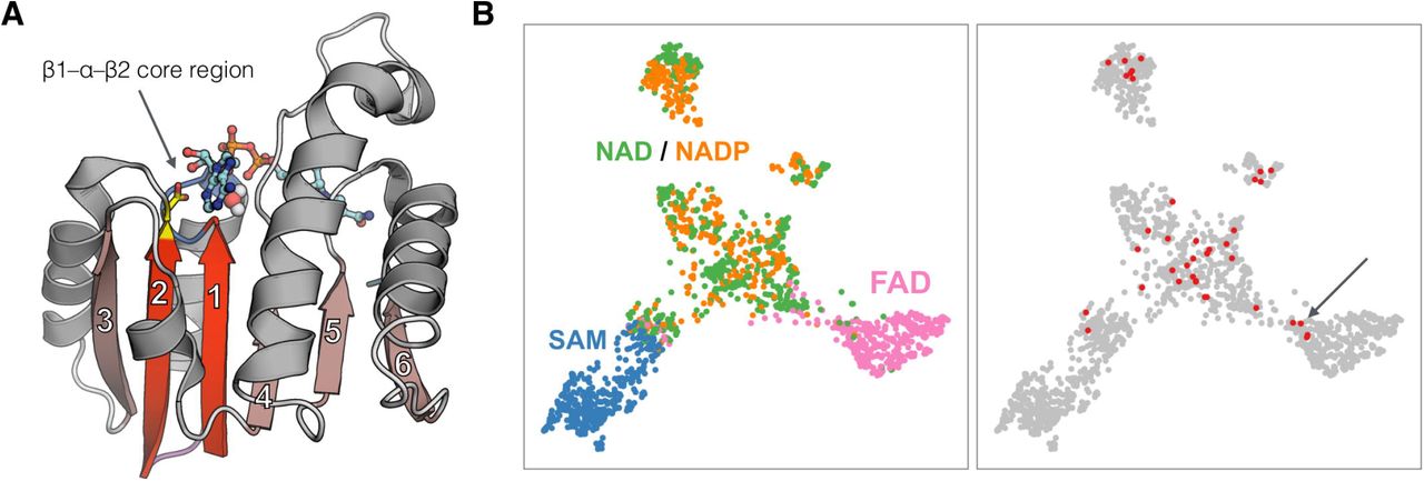
Cofactor recognition in Rossmann fold proteins. (A) Example of Rossmann fold protein, the malate dehydrogenase from Escherichia coli bound to NAD cofactor (shown as a ball-and-stick model). Beta strands are numbered according to the topological order and the two of them that form the cofactor-binding core are indicated with a brighter color. The aspartic acid residue essential for the cofactor binding is shown in yellow. (B) Sequence-based clustering of Rossmann core regions used to train and test the two prediction models. Points correspond to 1,647 core regions and their positions reflect the relative sequence similarity. The left panel depicts core regions colored according to the bound cofactor type, whereas the right panel highlights core regions (shown in red) used for benchmarks based on experimental data.

The NAD, NADP, and FAD cofactors are essential for the functioning of oxidoreductases, whose role is to transfer electrons from one molecule (electron donor) to another (electron acceptor). For example, alcohol dehydrogenases facilitate the oxidation of alcohol (electron donor) to aldehyde with the concurrent reduction of NAD+ (electron acceptor) to NADH. Generally, NAD occurs mostly in catabolic reactions, i.e., reactions that lead to the decay of complex molecules, and as a result, produce energy, whereas NADP (differing from NAD only by an additional phosphate group) is involved mostly in anabolic reactions, which create complex molecules from simple substrates and thus store energy. The addition of the phosphate in NADP does not alter its electron transport capability; however, the phosphate group modifies the structure of the cofactor, which allows different enzymes to have different specificities for NAD and NADP, thereby decoupling the catabolic and anabolic reactions (6). In contrast to NAD(P) and FAD, SAM takes part in methylation reactions, i.e., transferring a methyl group from SAM to substrates like DNA/RNA, proteins, or small-molecule secondary metabolites (7), and in other pathways such as these of the polyamine biosynthesis (8).

The rational cofactor specificity re-engineering is used for manipulating metabolic pathways (9, 10), and it has applications in drug engineering and industry (6). One of the first attempts to redesign the cofactor specificity of a Rossmann-like enzyme was a work by Scrutton and colleagues (11). By investigating the Escherichia coli glutathione reductase, the authors identified amino acids that confer specificity for NADP and then systematically replaced them to achieve cofactor preference gradually switched towards NAD, while preserving the specificity towards the substrate. To this date, there were many other successful attempts to rationally change the cofactor specificity of Rossmann enzymes (12); however, most of them were based on experimental or theoretical structures of the target protein and/or a detailed sequence alignment among the family members (13–15). These successful cases of NAD to NADP and vice versa conversions were the basis for the formulation of rules defining how properties of amino acids located at the cofactor-recognizing site dictate its binding specificity (16). The extensive research on the cofactor specificity determinants has led to the development of universal computational models. For example, Cui et al. proposed an approach in which molecular dynamics simulations were used to evaluate mutants based on their propensity to form hydrogen interactions with a cofactor (17). A structure-based strategy was also employed in CSR-SALAD, a method that aids the selection of amino-acid positions for the site-saturation mutagenesis (18). Cofactory is the only available computational tool capable of high-throughput, sequence-based evaluation of Rossmann enzymes for their ability to bind NAD, NADP, and FAD cofactors (19). However, the method does not consider SAM, and its accuracy is far from satisfactory, especially in the case of NADP-preferring proteins.

Obtaining accurate predictions for a wild-type sequence and its potential variants is a prerequisite for cofactor re-engineering tasks. However, performing such analyses with the currently available approaches requires time-consuming, case-by-case investigation of relevant sequences, structures, and literature. To address this problem, we collected all known experimental structures of the Rossmann fold proteins complexed with cofactors and used this data to train deep-learning-based models for the prediction of the cofactor specificity in Rossmann enzymes based on the sequence or structure of the βαβ core region. We rigorously tested the methods using a test dataset comprising examples sharing no more than 30% sequence identity to the dataset used for the training and a panel of 38 experimentally confirmed transitions between NAD and NADP enzymes. Both benchmarks revealed outstanding accuracy of the models and their applicability to re-design tasks.

Methods

Training Data Preparation

From 44 manually-selected Rossmann structures (Supplementary Table 1), we extracted Cɑ atoms corresponding to 3-2-1-4-5 β-sheets and the α-helix connecting β1 and β2. Such partial backbone structures were used to search the Protein Data Bank (PDB) using the MASTER tool (20). The resulting matches were processed using Python scripts to obtain fragments corresponding to the βαβ core regions responsible for the cofactor binding. For handling the structures, we used Atomium (21) and localpdb (Ludwiczak et al., https://github.com/labstructbioinf/localpdb, manuscript in preparation). The core fragments were analyzed with the PLIP tool (22) to identify protein-cofactor interactions, and all the cores lacking such interactions were discarded. The resulting set of 11,487 βαβ cores bound to cofactors was the basis for constructing training, validation, and test sets for use in machine learning. First, all the core sequences were clustered with mmseqs2 (23) (min. sequence identity 0.3, coverage 0.5, coverage mode 1, clustering mode 2), yielding 483 clusters comprising 1,647 unique cores (Figure 1B). Initially, all the clusters were assigned to the training set, and then they were randomly moved one by one to the test set to achieve a balance within the training set (the equal number of examples for each cofactor class) and between the training and test sets (70% of cores in each class belonging to the training set). Subsequently, the test set was further subdivided into test and validation sets. To this end, an analogous procedure was used in which clusters were randomly moved from the test set to the validation set while assuring the same distribution of examples within classes (Supplementary Figure 3).

Sequence-based approach

All sequences from the aforementioned non-redundant set of 1,647 cores were embedded with the SeqVec method (24), resulting in the vectors of size [N, 1024] (where N is the length of the core sequence). Neural network architecture was adopted, with minor modifications, from the original SeqVec paper (24), which described several applications of the embeddings for sequence classification tasks. Briefly, the SeqVec embeddings were processed by two consecutive convolutional layers and connected through two densely connected layers to the sigmoid-activated 4-class output layer denoting the binding probability for each of the cofactor classes. Batch normalization and random dropout (probability 0.5) operations were applied after each convolutional layer to avoid overfitting. Individual model training was performed for 50 epochs with the cross-entropy loss function, one-hot encoded labels derived from the structural data (see the preceding section for the details), and the Adam optimizer (25) as implemented in the tensorflow Python package. Input vectors were centered and zero-padded to the constant length of 65. Models weights were saved from the epochs corresponding to the highest macro-F1 score on the validation set. To increase the model diversity and further improve the calibration, we trained a total of 250 models using the above procedure and randomly varying the following parameters – a) maximum sequence identity in the training set (from 0.3 to 0.9 in 0.1 intervals), b) sequence coverage used to calculate sequence identity (from 0.5 to 0.8 in 0.1 intervals), c) amount of the noise applied to the labels (from 0 to 0.2 in 0.05 intervals, where the numbers denote the standard deviation of the zero-centered normal distribution from which the random noise samples were drawn from; individual labels were clipped to the original [0, 1] range after this operation), and d) batch size used during the training (from 8 to 40 in 8 samples intervals). The top 10 models, exhibiting the highest macro-F1 scores on the validation set, were used to create the final ensemble, which averages the outputs of these best-performing models. The per-residue contributions to the predicted cofactor binding classes were calculated using the captum Python package with the integrated gradients method (26) implemented therein. Exact network implementation, requirements, and scripts allowing to perform inference are available through the code repository accompanying the manuscript (https://github.com/labstructbioinf/rossmann-toolbox).

Structure-based approach

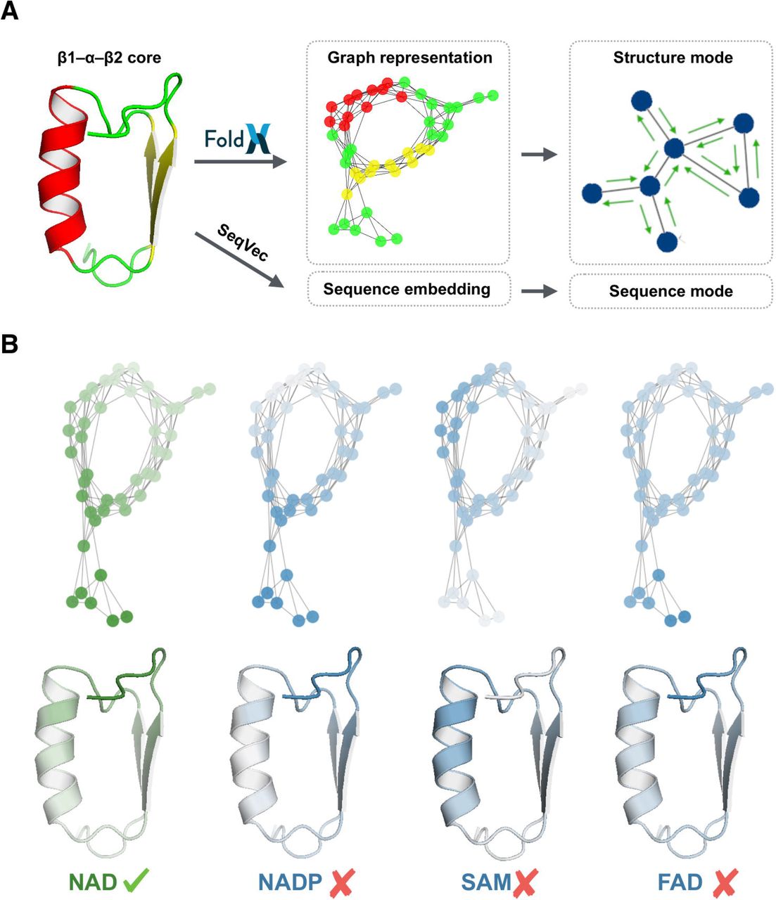
Graph neural networks (GNNs) are extensions of regular neural networks to operate on graph-structured objects. They allow for a more natural representation of complex non-grid data, such as protein structures. An undirected graph G is defined as a set of nodes N, also termed vertices, n ∈ N, and a set of edges E; if two vertices are connected by an edge then e_ij = e_ji ∈ E. A graph can also be represented as an adjacency matrix A = {a_ij} sized |N| x |N|, where |N| denotes the number of graph nodes. The core structures from the training, validation and test sets were converted to graphs (Figure 2A) in which nodes represent the individual residues and edges define interactions between them (two residues were considered to be interacting when the distance between their Cɑ atoms was below 7 Å). Subsequently, nodes and edges of the resulting graphs were annotated with precise structural data. To this end, the full-length structures containing the core regions were minimized in the FoldX force field (27) using the RepairPDB command, and then the structural features were extracted with SequenceDetail and PrintNetworks commands and assigned to nodes and edges, respectively (Supplementary Table 3). Such a graph representation with nodes and edges filled with features constitutes the input to the network, whereas its output is a four-element vector reflecting the probability toward binding of the individual cofactors.

Figure 2.

General scheme of the prediction pipeline. (A) The pipeline consists of two prediction models, which enable the cofactor specificity prediction based on the sequence and structure of the βαβ core. (B) The prediction models return not only the binding probabilities but also per-residue importance scores reflecting the individual residues’ contribution to the final prediction. Colors ranging from green via white to blue indicate positive, neutral, and negative impact on a given prediction, respectively.

The GNN model was implemented in Deep Graph Library (28) using PyTorch backend and Lightning training routines. It is composed of a series of EdgeGAT layers blocks, where each block contains an EdgeGAT layer followed by a batch normalization layer (edges and nodes are treated separately) with LeakyReLU activation function. To transform graphs of various sizes to a fixed-size representation, the last EdgeGAT layer produces the output with node features of size 4 (i.e., number of cofactors), which are subsequently summed over the graph and passed through the fully connected layer followed by the Sigmoid activation function. The two main hyperparameters of the network are the number of internal EdgeGAT blocks and the size of the node features vector (the edge features size was fixed at 20). For the training, the focal loss cost function (29) and Adam optimizer (25) with L2 regularization were used. Training stopping criteria were given by not increasing the F1-macro score over the validation set. All training parameters are supplied in the attached repository (https://github.com/labstructbioinf/rossmann-toolbox). In total, we trained 1,400 models with various hyperparameter values (two or three EdgeGAT blocks and the size of node features ranging from 128 to 512), and the four models that performed the best on the validation set were selected to build the final structure-based model.

The limitation of the current GNN architectures in the context of processing molecular data is their inability to jointly process information stored in nodes and edges (30). This feature is essential for obtaining a complete graph representation of a protein structure in which residues (nodes) and interactions (edges) aren’t artificially separated. To address this problem, we decided to expand the Graph Attention Network (GAT) algorithm (31) with the possibility of handling complex edge features. The original GAT idea is to compute individual attention scores, known as edge weights, for each connection in the graph. The first step is to update node features with regular fully connected layer h′_i = Wh_i + b, where W and b are learnable parameters, and to calculate attention scores using where a_ij denotes attention score, that is normalized weight over connection n − n_j, ϵ_ij is the unnormalized weight where A is a learnable matrix, LeakyReLUis an activation function, and (· ||·) denotes vector concatenation operation. After obtaining the attention of each connection, updated feature vector h^″_i of node n_i is calculated with the equation In this way, the individual GAT layers will learn which connections are important with respect to the information stored in n_i and its neighbors. However, in such an implementation, the edge feature is only temporary and it is not propagated further through the network. Our extension (Figure 3) replaces equation (2) with where F is learnable matrix and f′_ij are updated edge features produced by in this case, the concatenation (· ||· ||·) is performed over three quantities h′_i, h′_j, and f_ij. We decided to not use the resulting output edge features in the last EdgeGAT layer (in this case Eq. 4 is replaced with ϵ_ij = f′_ij). The flow of the calculations is presented in Figure 3 and can be summarized in four steps:

1. calculate auxiliary node feature vector h′_i (Figure 3A)

2. use node (h′_i and h′_j) and edge features (f_ij) for each existing connection in a graph to calculate output edge features f′_ij (Figure 3B)

3. use output edge features f′_ij to calculate each edge attention α_ij /ϵ_ij – connection importance factor. Note that importance coefficients are also calculated for self-loop edges connecting nodes with themselves (not shown in Figure 3C).

4. sum node features h′_ij multiplied by their importance factor to obtain output node features h^″_i. Owing to the usage of self-loops (see above), in cases when all the surrounding connections are irrelevant (attention score equals zero) then the new state h^″_i will be the same as the old one h′_i (Figure 3D).

Figure 3.

Schema of a single Edge-GAT layer. For the sake of clarity, only some nodes and edges are annotated. (A) An exemplary input network comprising four nodes and three edges. h′₁ and h′₂ denote updated features (with regular fully connected) of nodes 1 and 2, respectively, whereas f₁₂ denotes features of the edge that connects them. (B) Concatenation of node and edge features and calculation of updated edge features (f′₁₂). (C) The updated edge features are used to calculate the importance (a value between 0 to 1) of node-edge-node connections (a′₁₂). A new node feature (h^′′₂) is calculated as an average of surrounding node features weighted by the importance factors (a′). Note that the h^′′₂ is also used; its weighting importance factor is calculated from a self-loop edge feature (f′₂₂). The self-loops were omitted for clarity. (D) Final output network with updated node and edge features.

Experimental benchmark set

Literature mining revealed 38 experimentally confirmed cases of switching the cofactor specificity of Rossmann fold enzymes from NAD to NADP and vice versa (Supplementary Table 2). To verify whether the benchmark set is representative and not biased towards certain types of proteins, we performed clustering of all its sequences together with the sequences from the train-test-validation set. To this end, we calculated a SeqVec (24) embedding for each core sequence, compared them in all vs all fashion using cosine similarity metric, and used the resulting matrix as an input to the UMAP dimensionality reduction procedure. The results were visualized as 2D plots (Figure 1B), revealing the representativeness of the benchmark sequences.

Prediction benchmark

All the predictions were performed with Cofactory (19) and the two methods developed in this study. Sequences were used as inputs for Cofactory and the embedding-based predictor, whereas the PDB structures or FoldX (27) models were used as inputs for the structure-based predictor. We also built a simple consensus classifier in which predictions from the two methods were combined using an F1-like formula: 2 * structural_score * sequence_score / (structural_score + sequence_score). The performance of the individual methods was estimated using the test set (Figure 4) and a separate test set (Supplementary Table 2) comprising experimentally confirmed cases (Figure 5). In the latter benchmark, we calculated the ΔNAD and ΔNADP for each WT-mutated cores pair. These scores, reflecting the change in the predicted binding probabilities upon mutation, were used to calculate the Δacc coefficient defining the number of the benchmark cases in which the direction of the change was predicted correctly (Figure 5). In addition, a prediction accuracy (acc) for all WT cores was calculated (the mutated variants were not considered because some of them may bind both cofactors).

Figure 4.

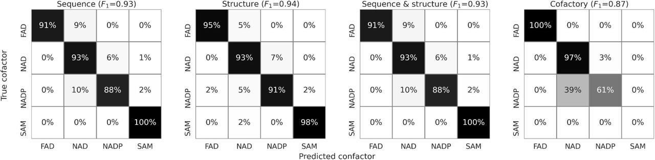
Performance of the prediction models on the test set comprising βαβ cores showing no more than 30% sequence identity to the training set. The SAM cofactor was omitted in the case of Cofactory since this method does not support predictions for this cofactor.

Figure 5.

Performance of on the test set comprising 38 experimentally confirmed cases of altering the cofactor specificity between NAD and NADP. ΔNAD and ΔNADP denote the difference between predicted binding probabilities of WT and mutated sequences.

Brute-force mutational scan

For each of the 38 WT cores from the experimental benchmark set (Supplementary Table 2), all possible point mutations were defined and their structures were modeled with Modeller (32) and FoldX (27). Subsequently, the affinity of the resulting variants towards NAD and NADP cofactors was predicted with Cofactory (19) and the consensus classifier (see above). The most plausible variants, i.e., those which may change the cofactor specificity in the assumed direction, were selected using the following procedure. First, possibly unstable models characterized by FoldX ddG score or Modeller DOPE score greater than 4.5 and 240, respectively, were discarded. Then, the raw consensus scores for NAD and NADP were adjusted by multiplying them by the corresponding attention scores (the per-residue contributions) associated with the position where a given mutation was introduced. Finally, for each benchmark case, all the mutants were sorted according to the adjusted consensus scores, and the positions of experimentally confirmed mutants were indicated (Figure 6A).

Figure 6.

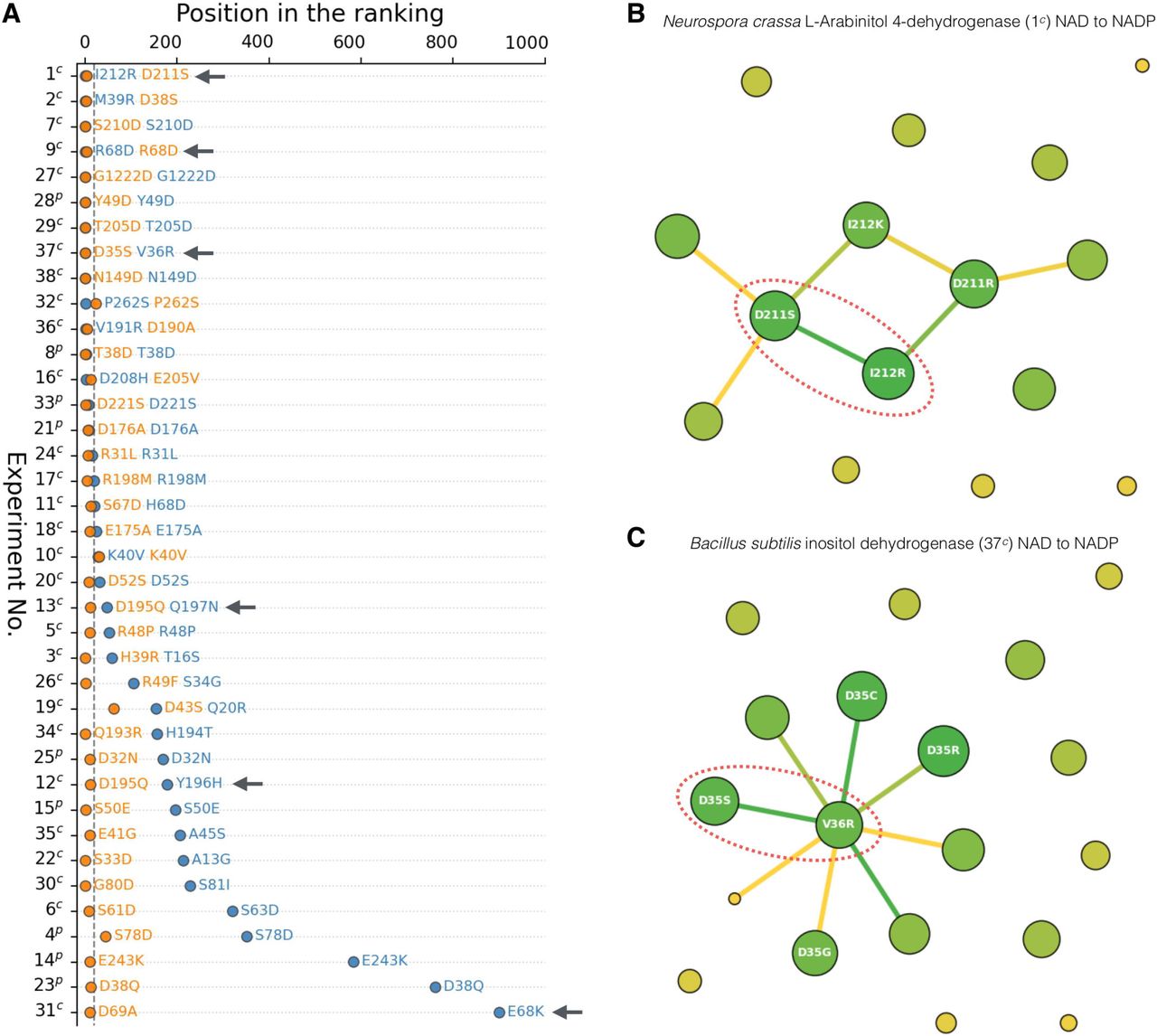
Performance of the consensus approach and Cofactory in the task of cofactor specificity design. (A) Results of the brute-force mutational scan of the 38 cores from the benchmark set (Supplementary Table 2). Rows correspond to the 38 experiments in which the specificity change of Rossmann enzymes was achieved by either point or complex (double, triple, etc.) mutations (“p” and “c” suffixes, respectively). Orange and blue circles indicate positions of the experimentally confirmed mutations in the rankings of all possible point mutations ordered according to the score of a given method (the consensus approach and Cofactory, respectively) – the lower the position, the better performance. In experiments relying on complex mutations, only the best-scored mutation is shown. (B) Result of the iterative mutational scan of L-Arabinitol 4-dehydrogenase. Circles denote mutations (their sizes are proportional to the frequency of occurrence), whereas edges between them define predicted coupling (the more green is an edge, the more probable is the given coupling). Experimentally confirmed pairs of mutations are indicated with red ovals. (C) Result of the iterative mutational scan of inositol dehydrogenase.

Iterative mutational scan

For the identification of the complex mutations, that are composed of more than one point mutation, an iterative mutational scan was performed employing the sequence-based method and Monte Carlo heuristics. In the implemented approach, the state of the system is fully described by the N point mutations (substitutions) applied to the WT sequence. In a single simulation step from 1 to N mutations are randomized (by changing their position and substituting amino acids), and a new resulting sequence is evaluated with the sequence-based prediction model. A new state of the system is accepted according to the Metropolis criterium with the probability calculated with the following formula: where S_N is the score of a sequence obtained in the given simulation step and S_B is the score of the sequence obtained with the set of the currently best-performing mutations.

The convergence of such computations can be further enhanced with the use of modified probability distributions during the randomization procedure. The positions in the sequence can be chosen according to the per-residue contributions to the prediction of the desired cofactor, whereas the choice of amino acid in a given position can be modified by the use of PSSM scores derived from multiple sequence alignment (MSA) of cores binding the desired cofactor (for the MSA calculation we used parMATT (33)).

The simulation can be described with 3 parameters: 1) the number (N) of point mutations introduced to the WT sequence, in the range from 1 to 5, 2) whether or not the enhanced probability distributions were used, and 3) kT value: 0.05 or 0.1. For each of the 38 WT cores from the benchmark set, we have performed a parameter scan employing 50 replicated simulations in each specification. This resulted in a total of 1000 simulations, each lasting 500 steps, being performed for every WT core.

The results were evaluated to find the best performing mutations for each core of the benchmark set (Supplementary Table 2) and compare them with the experimental results. To this end, for each benchmark case, sequences from all simulation steps were binned based on the actual number of mutations relative to the WT. In each group, the 95th percentile of the score was defined and variants with scores below this value were discarded. The remaining sequences from all bins were collected and the 20 most frequent point mutations were determined (in the case of sequences containing more than one mutation, each was treated separately). Such a list was then filtered by removing variants with FoldX ddG score above 4.5 or Modeller DOPE score above 240 (3D models were previously calculated in the brute-force procedure), and sorted by the frequency of the individual mutations. An analogous procedure was used to determine the most frequently occurring pairs of mutations. In this case, all the variants that remained after FoldX and Modeller filtering were analyzed to determine co-occurring mutations (in the case of variants containing more than two mutations, all possible combinations were considered regardless of the relative position in the sequence). Then, the pairs not involving the mutations from the previously defined top 20 list were removed and the remaining ones were sorted according to their frequency, resulting in a ranking of mutations’ co-occurrence.

Results and Discussion

Defining the minimal cofactor specificity-defining region

The most conserved and essential interactions between the Rossmann fold proteins and their cofactors occur in the core region corresponding to the βαβ motif (Figure 1A) (4). Consequently, mutating the residues in this region is typically sufficient to alter the cofactor specificity (Supplementary Table 2). To gain insight into whether the core region sequences contain enough information to discriminate between cofactors they bind, we performed clustering analyses (Figure 1B). A clear separation between SAM, FAD, and NAD(P)-utilizing enzymes was visible; however, the latter group was mixed, and the NAD and NADP-utilizing enzymes were not separable. This result suggests monophyletic origins of SAM and FAD-binding cores and confirms the well-known observation that the transitions between NAD and NADP specificity have occurred multiple times (what is to be expected, considering that even single point mutations are capable of inducing such a change). Given the above observations, we assumed that the sequence and structure of the βαβ region are sufficient for the prediction of cofactor binding specificity.

Deep learning-based prediction of the cofactor specificity

We considered two complementary approaches to tackle the problem of cofactor specificity prediction in Rossmann fold proteins. Both rely on deep learning procedures but differ in terms of the neural network architectures and data type used. The first of the methods uses only sequences of cofactor-binding cores, whereas the second also employs the structural data represented in the form of graphs. We constructed a data set comprising 1,647 unique Rossmann cores divided into training, validation, and test sets and used it to develop the two methods. While the first two sets were used for training and selecting the best models, the third, comprising βαβ cores showing no more than 30% sequence identity to the cores from other sets, was used for estimating the effectiveness of the methods. Both methods achieved excellent accuracy (93% and 94%) and outperformed the only currently available method, Cofactory, especially in predicting the NADP-specific cores (Figure 4). We attribute the rare cases of mispredictions, e.g., confusing NAD and NADP-binders, to the fact that our methods were trained using protein-cofactor complexes obtained from PDB, which may not be accurate in all cases. Moreover, some Rossmann enzymes recognize both NAD and NADP (14, 17, 34), but they may be present in PDB only in a single form. We attempted to identify such ambiguous cases in our data sets by performing molecular dynamics and docking simulations of the core-cofactor complexes, though without success (data not shown).

Finally, we found that although the accuracies of the sequence- and structure-based models are comparable, their predictions differ, especially in the most uncertain cases (Supplementary Figure 1). Such a partial lack of correlation indicates that, to some extent, the methods must have captured different aspects of the cofactor specificity determinants. Considering this, we built a consensus classifier (see Methods) in which the predictions from two methods were combined (Figure 4).

Benchmark using experimental data

Despite the excellent performance on the test set, we deemed it necessary to validate our methods on more difficult, real-life examples. To this end, we built a benchmark set comprising 38 published experiments that aimed at switching the cofactor specificity from NAD to NADP and vice versa by introducing one or more mutations in the βαβ core region (Supplementary Table 2). Among these benchmark cases, we found mutations designed using various approaches ranging from loop exchange (35, 36), evolutionary-based (37) to computational predictions (17, 18). While the wild-type sequences of this set may have counterparts in the train set used for the development of the prediction models, their mutated variants were never “seen” during the training procedure, making the correct predictions more challenging. Like the benchmark with the test set, this benchmark also indicated the superiority of deep learning models developed in this study over Cofactory (Figure 5). The consensus approach achieved 100% accuracy (Δacc) in predicting the direction of cofactor specificity change upon mutation and 95% accuracy (acc) in predicting the preferred cofactor of the WT cores (we did not consider mutated sequences in the calculation of the acc coefficient because the increase in the affinity towards one cofactor does not necessarily imply the decrease in the affinity towards the other, and the resulting mutated enzymes may have dual specificity, e.g., (14, 17, 34); Supplementary Table 2).

There were only three cases in which one or more of our approaches failed to predict the cofactor specificity of the WT core correctly. The first one, dihydrolipoamide dehydrogenase (position 16 in the benchmark set; Supplementary Table 2), an E3 component of the pyruvate dehydrogenase complex (38), contains two Rossmann fold domains, both belonging to the FAD/NAD(P)-binding group defined in the ECOD database (39). The first domain is involved in FAD binding, whereas the second recognizes NAD. The proposed mutations (40) aimed at switching the cofactor specificity of the latter domain to NADP. The sequence, structure, and consensus approach correctly predicted the effect of these mutations (probability of NADP binding changed from 0.0 to 0.35-0.7, depending on the method); however, all of them predicted the WT core to bind FAD with a high probability of 0.7-0.8. The second mispredicted case, water-forming Streptococcus mutans NADH oxidase (position 36 in the benchmark set), has the same domain composition as the dihydrolipoamide dehydrogenase and contains two Rossmann domains from the FAD/NAD(P)-binding group. In this case, also the second Rossmann domain was mutated (41), and the direction of the resulting cofactor specificity change was predicted correctly (probability of NADP binding changed from 0.0 to 0.5-0.8), but the WT variant obtained the highest score for FAD instead of NAD (in this case, however, only the structure-based method yielded such an unexpected result). The fact that in both cases the FAD score exceeds the NAD score can be attributed to the evolutionary position of the respective βαβ core domains. Both, despite being experimentally confirmed NAD binders, cluster together with FAD-bound βαβ cores (Figure 1B) and thus may constitute an example of the specificity switch within the FAD/NAD(P)-binding group. Since such cases are rare in our dataset (especially compared to the NAD–NADP transitions), they may have been missed during the training process. The last mispredicted case, the flavoprotein monooxygenase can use non-phosphorylated cofactor NAD, as well as NADP, for the reduction (42), thus it is not surprising that the prediction for its WT core was ambiguous. However, also in this case the direction of specificity change upon mutation was predicted correctly.

Brute-force and iterative mutational scans

In the benchmark described above, we estimated the ability of the methods to predict the cofactor specificity and its changes upon mutation correctly. In such cases, however, both the wild-type and mutant sequences are known. To mimic real-life scenarios in which the cofactor-switching mutations of a given wild-type core region are predicted from scratch, we reached for two approaches: one relying on the evaluation of all possible point mutations (brute-force approach) and the other employing Monte Carlo heuristic to identify complex variants in which more than one position is altered (iterative approach).

To test the brute-force approach, each WT sequence of the benchmark set (Supplementary Table 2) was used as a starting point to generate all possible point mutations (19*n, where n is the length of the core region). For each benchmark case, the calculated point mutations were evaluated with the individual methods, sorted according to the predicted affinity towards the desired cofactor, and the position of the “correct” mutation, i.e., the one described in the respective publication, was indicated (Figure 6A). In this way, we obtained an estimate of how efficient are the individual methods in de novo prediction of cofactor-switching mutations – the lower is the position of the “correct” mutation, the fewer lab experiments would have been necessary to reveal them (later in the text, we define such a “correct” variant as properly predicted whenever it occurs among the 20 top-scored mutants; see dashed vertical line on Figure 6A).

The benchmark set can be divided into two groups; the first one encompasses cases where the switch of the specificity was obtained with a single substitution (nine cases indicated with “p” in Figure 6 and Supplementary Table 2), whereas the second contains those involving two or more substitutions to the WT core (29 cases indicated with “c”). In the first group, the consensus approach and Cofactory properly identified the “correct” mutation in eight and four cases, respectively, whereas in the second group in 26 and 13 cases, respectively. Among the cases of the second group, six relied on a multi-step approach in which mutations were gradually added and tested experimentally to obtain increasing specificity towards the desired cofactor (1^c, 9^c, 12^c, 13^c, 31^c, and 37^c; indicated with arrows in Figure 6A). For example, the study aiming at switching the cofactor specificity of L-Arabinitol 4-dehydrogenase (1^c) from NAD to NADP (43) involved multiple rounds of rational design. The D211S variant obtained at the first round showed a decrease in activity towards NAD, with a minimal yet detectable activity increase towards NADP, whereas the second-round double mutant D211S/I212R displayed actual reversal in cofactor specificity. The brute-scan approach identified the first-round D211S variant with the highest confidence (first position in the ranking; Figure 6A). Intrigued by this observation, we investigated the remaining cases and found that in all but one of them (9^c) the predicted mutation corresponded to the first one predicted by a given experimental protocol. The above results indicate that the brute-force scan is suitable for de novo prediction of point mutations that result in a complete or partial switch of the specificity towards the given cofactor.

Using a brute-force approach for the identification of complex mutations involving more than one position would be computationally infeasible. To address this problem, we have developed an iterative approach capable of simultaneous prediction of more than one mutation by altering positions indicated by the neural network rather than exhaustively evaluating all the possible variants. In contrast to a brute-force scan, the iterative approach returns not only a ranking of specificity-switching mutations but also of their co-occurrences. For example, in the case of the aforementioned L-Arabinitol 4-dehydrogenase (1^c) the D211S mutation indicated by the brute-force scan was predicted to co-occur with two mutations I212K and I212R (Figure 6B), and the one showing the strongest coupling (I212R) was also confirmed experimentally (43). Another example was the reengineering of the cofactor specificity of Bacillus subtilis inositol dehydrogenase (37^c) from NAD to NADP (Figure 6C). In this case, our predictor identified the coupling between two out of three mutations (D35S and V36R) that were previously suggested in the experimental study (15). The third mutation, A12K, was not predicted; however, it must be noted that the double mutant D35S/V36R already preferred NADP over NAD by a factor of 5. In fact, the A12K mutation was not essential, and its purpose was to improve the specificity change further. Inspection of all 29 benchmark cases featuring two or more mutations revealed that in 15 of them the iterative approach predicted more than one “correct” mutation, and in 8 out of these 15 cases also the “correct” coupling between them (Supplementary Table 4). It is important to note that the “correct” mutations obtained from the experimental studies aren’t necessarily the only ones that are capable of inducing the specificity switch, and it is possible (considering the very good performance of the methods; Figures 4 and 5) that the top-scored predictions may constitute alternative solutions.

Conclusions

While the presented methodology shows excellent performance, there is still room for improvement. We have identified the three most important areas where further studies could help make it even better. First, our methods were trained only with natural βαβ cores obtained from PDB. This, in turn, can make them prone to assign good scores to cases that are meaningless from the structural perspective. This problem was partially overcome by utilizing Modeller and FoldX energy estimates to detect and discard potentially unstable variants. However, a more elegant solution would be introducing such variants to the training set and marking them as non-binders. Second, sequence embeddings and graph neural networks are relatively new tools, and their applicability to biological tasks are still being explored. In this study, we not only demonstrated their usefulness in the prediction of protein-ligand interactions but also developed new solutions such as the EdgeGAT layer (Figure 3), substantially expanding the applicability of GNNs in structural biology (30). Thus, we plan to develop this methodology further to extend its applicability to other related tasks. Finally, in our benchmarks, the two approaches turned out to provide somewhat similar results; however, we believe that their potential is yet to be explored by the researchers. For example, we envision that for complex reengineering tasks, such as a switch between NAD(P) and SAM, it may be necessary to use structural descriptors that are capable of capturing subtle structural differences (44) and pinpointing essential regions (Figure 2B). Bearing in mind the possibility of designing such a transformation, we noted that some of the NAD(P)-binding βαβ cores are localized at the boundary of the SAM group (Figure 1B; Supplementary Figure 2). Such borderline cases may constitute a good starting point for such new experiments.

Authors’ contributions

SDH, KK, and JL designed the study. SDH, KK, JL, RM, and KS prepared the datasets. KK designed and implemented the graph-based prediction model, whereas JL designed and implemented the embedding-based prediction model. MJ and AB designed and implemented the MC-based mutational scan. KS implemented the webserver. SDH, KK, JL, and MJ drafted the manuscript. All authors read and approved the final version of the manuscript.

Acknowledgments

This work was supported by the First TEAM program of the Foundation for Polish Science co-financed by the European Union under the European Regional Development Fund (grant POIR.04.04.00-00-5CF1/18-00 to SDH). JL was in part funded by the National Science Centre (grant 2017/27/N/NZ1/00716 to JL). The authors would like to thank Paola Laurino, Saacnicteh Toledo Patino, and Vikram Alva for their constructive comments and critical evaluation of the manuscript.

Footnotes

• https://github.com/labstructbioinf/rossmann-toolbox

• https://lbs.cent.uw.edu.pl/rossmann-toolbox