

Summary
Voluntary movement requires communication from cortex to the spinal cord, where a dedicated pool of motor units (MUs) activates each muscle. The canonical description of MU function, established decades ago, rests upon two foundational tenets. First, cortex cannot control MUs independently1 but supplies each pool with a common drive that specifies force amplitude2,3. Second, as force rises, MUs are recruited in a consistent order4–13 typically described by Henneman’s size principle14–19. While this paradigm has considerable empirical support, a direct test requires simultaneous observations of many MUs over a range of behaviors. We developed an isometric task that allowed stable MU recordings during rapidly changing force production. MU responses were surprisingly flexible and behavior-dependent. MU activity could not be accurately described as reflecting common drive, even when fit with highly expressive latent factor models. Neuropixels probe recordings revealed that, consistent with the requirements of fully flexible control, the cortical population response displays a surprisingly large number of degrees of freedom. Furthermore, MUs were differentially recruited by microstimulation at neighboring cortical sites. Thus, MU activities are flexibly controlled to meet task demands, and cortex has the capacity to contribute to that ability.
Primates produce myriad behaviors, from acrobatic maneuvers to object manipulation, all requiring precise neural control of muscles. Each muscle is controlled by a motor neuron pool containing hundreds of anatomically and functionally diverse motor units (MUs)20. One MU is defined as a spinal ɑ-motoneuron and the muscle fibers it uniquely innervates21. MUs are highly heterogeneous22, differing in size (large MUs innervate more fibers), duration of generated force22, and the muscle length where force is maximal23.
Optimality suggests using MUs best suited to the specific situation24. Yet such flexibility would necessitate non-trivial computational resources, including participation by brain areas aware of the full movement and context. A simpler alternative is a spinally implemented recruitment strategy that approximates optimality in limited contexts. Supported by nearly a century of research, this alternative has become the canonical conception of MU control1,25. In decerebrate cats, MUs are recruited and de-recruited in a consistent order26 from smallest to largest according to Henneman’s size principle14–19. Orderly MU recruitment is similarly observed following supraspinal stimulation in cats27 and during voluntary muscle contractions in humans4–13. MU firing rates increase monotonically with force and display correlated fluctuations2, arguing that MUs are jointly controlled by a one-dimensional (1D) ‘common drive’3. This ‘rigid control’ hypothesis -- common drive followed by small-to-large recruitment -- is codified in standard models of muscle activation28,29.
Rigid control is believed to relieve cortex from the burden of controlling MUs independently3,18. Small-to-large recruitment minimizes fluctuations during constant force production and is thus optimal in that context30–32. In idealized form, rigid control describes each muscle and its MU pool. There are known exceptions24,33–36 when a ‘multifunctional’ muscle pulls in different directions (necessitating more than one common drive24,35) or drives movement across two joints and participates in multiple synergies33. These properties are compatible with rigid control under an operational definition of an MU pool37–39; descending commands can remain simple (specifying force direction24 or synergy activation33) and small-to-large recruitment holds for any given force direction.
The alternative to rigid control is highly flexible MU recruitment that adapts to situational demands. Some flexibility has been observed during locomotion40,41, where it may reflect the need to control force when a muscle lengthens under load34,42,43. It also seems intuitive that recruitment should favor fast-twitch MUs when forces change rapidly. Yet it remains controversial whether speed does39,44,45 or should46 influence recruitment.
Rigid control is thus believed to govern the vast majority of cases46, with exceptions being rare and/or inconsistent across studies39,45. An accepted caveat is that critical tests have yet to be performed39. Due to the difficulty of recording many MUs during swiftly changing forces44, no study has directly addressed the key situation where rigid and flexible control make divergent predictions: when a subject skillfully performs diverse movements, is MU recruitment altered to suit each movement? An additional key test also remains. Fully flexible control would require, in addition to spinal mechanisms, some influence from areas aware of overall context. Flexible control thus makes the strong prediction that altering cortical activity should alter recruitment. This does not occur in cat27, but remains to be examined in primate.
Pac-Man Task and EMG recordings
We trained one rhesus macaque to perform an isometric force-tracking task. The monkey modulated force to control the vertical position of a ‘Pac-Man’ icon and intercept scrolling dots (Fig. 1a). We could request any temporal force profile by appropriately selecting the dot path. We conducted three experiment types, each using dedicated sessions. Dynamic experiments employed many force profiles including slow and fast ramps and sinusoids (Fig. S1). Muscle-length experiments (Fig. 1b) investigated whether MU recruitment reflects joint angle/muscle length, using a subset of force profiles. Microstimulation experiments (Fig. 1c) artificially perturbed descending commands using microstimulation delivered via a linear electrode array in sulcal primary motor cortex (M1).

Single-trial (gray), trial-averaged (black), and target (cyan) forces for one session of dynamic experiments. Vertical scale bars indicate 4 N. Horizontal scale bars indicate 500 ms. n denotes trial count.

(a) Dynamic experiments. A monkey modulated the force generated against a load cell to control Pac-Man’s vertical position and intercept a scrolling dot path. A variety of force profiles were used, a subset of which were also employed during muscle-length and microstimulation experiments. (b) Muscle-length experiments. The manipulandum was positioned so that the angle of shoulder flexion was 15° (long) or 50° (short). (c) Stimulation experiments. Intracortical microstimulation was delivered through a linear array inserted in sulcal motor cortex. (d) Behavior and MU responses during one dynamic-experiment trial. The target force profile was a chirp. Top: generated force. Middle: eight-channel EMG signals recorded from the lateral triceps. 20 MUs were isolated across the full session; 13 MUs were active during the displayed trial. MU spike times are plotted as circles (one row and color per MU) below the force trace. EMG traces are colored by the inferred contribution from each MU (since spikes could overlap, more than one MU could contribute at a time). Bottom left: waveform template for each MU (columns) and channel (rows). Templates are 5 ms long. As shown on an expanded scale (bottom right), EMG signals were decomposed into superpositions of individual-MU waveform templates. The use of multiple channels was critical to sorting during challenging moments such as the one illustrated in the expanded scale. For example, MU2, MU5, and MU10 had very different across-channel profiles. This allowed them to be identified when, near the end of the record, their spikes coincided just before the final spike of MU12. The ability to decompose voltages into a sum of waveforms also allowed sorting of two spikes that overlapped on the same channel (e.g., when the first spike of MU6 overlaps with that of MU10, or when the first spike of MU9 overlaps with that of MU5). Multiple channels also guarded against mistakenly sorting one unit as two if the waveform scaled modestly across repeated spikes (as occurred for a modest subset of MUs).
On each of 38 sessions, we recorded from multiple custom-modified percutaneous thin-wire electrodes closely clustered within the head of one muscle. Recordings were made from the triceps and deltoid (dynamic experiments); deltoid (muscle-length experiments); and triceps, deltoid, and pectoralis (microstimulation experiments). It is notoriously difficult to spike sort EMG signals during dynamic tasks; movement threatens recording stability and vigorous muscle contractions cause MU action-potential waveforms to superimpose47. Three factors enabled us to identify the spikes of multiple single MUs, even during high-frequency force oscillations (Fig. 1d). First, the isometric task facilitated stable recordings even when force changed rapidly. Second, activity intensity could be titrated via the gain linking force to Pac-Man’s position. Finally, a given MU typically produced a complex waveform spanning many channels (Fig. 1d, bottom), which we identified by adapting recent advances in spike sorting48–50, including methods for resolving superimposed waveforms49 (Supp. Materials).
We isolated 3-21 MUs in each session (356 total units). Analyses considered only simultaneously recorded neighboring MUs, for two reasons. First, many of our recordings were from the deltoid, where different regions pull in different directions and physically distant MUs thus have different ‘preferred force directions’24. Second, across-session behavioral variability could conceivably make recruitment order appear inconsistent in pooled data. We thus compared only amongst simultaneously recorded neighboring MUs within a single muscle head, with all forces generated in one direction.
Motor unit activity during behavior
Rigid control applies to the behavior of the full MU pool, yet provides constraints that can be visualized at the level of MU pairs. MUs should be recruited in a consistent order16,18 and changes in their activity should not be strongly opposing5,12. Responses of MU pairs were typically consistent with these predictions during gradually changing forces at a single muscle length. For example, in Fig. 2a, MU88 is recruited before MU90 and the activity of both increases monotonically with increasing force. Both become less active as force decreases, with MU88 de-recruited last. The predictions of rigid control sometimes held during swiftly changing forces (Fig 2b). However, violations were common when comparing rapidly and slowly changing forces. For example, in Fig. 2e, MU309 is more active during the sinusoid (left) than during the ramp (right), while the opposite is true for MU311. Thus, which of the two MUs contributes the most to force production depends on context.

Each panel displays the trial-averaged force (top), mean firing rate with standard error (middle) and spike rasters (bottom) for a pair of concurrently recorded MUs during dynamic (a-e), muscle-length (f,g), and stimulation (h-j) experiments. Vertical scale bars indicate 8 N (forces) and 20 spikes/s (firing rates). Horizontal scale bars indicate 250 ms. Columns within panels correspond to different conditions. In h-j, labels indicate the stimulation electrode. Bars (with shaded region overlapping rasters) indicate stimulation duration. On average (across all sessions and experiments) each condition consisted of 34 trials on average.
Recruitment incompatible with rigid control also occurred within individual conditions if force changed at different rates during different epochs. In Fig. 2c, MU109’s activity rises threefold in anticipation of sudden force offset, even as MU108’s activity declines. In Fig. 2d, over the last three cycles of a chirp force profile, MU324’s activity decreases as MU329’s activity increases. These examples are inconsistent with common drive, which cannot simultaneously increase and decrease. For both pairs, the key violation (activity decreasing for one MU while increasing for another) was not observed when holding a static force. Instead, activity reflected whether forces were, or soon would be, rapidly changing. Yet it was rarely the case that MU activity simply reflected the derivative of force. The rate of MU109 (Fig. 2c) rises while force is constant. And while MU329 (Fig. 2d) and MU309 (Fig. 2e) are more active during higher-frequency forces, they do not phase lead their neighboring MUs. Activity reflecting not just force, but the overall situation, was particularly evident with changes in muscle length, both when activity was swiftly changing (Fig. 2f) and when it was static (Fig. 2g). Changes in recruitment with muscle length could be large (e.g., an MU becoming inactive for a given posture) but could also be more modest, allowing us to confirm recording stability (Fig. S2).

(a) Firing rate of a pair of simultaneously recorded deltoid MUs plotted against each other for three different conditions (columns) with the deltoid in a lengthened (blue) or shorted (red) posture. (b) Left. Template of MU157 across the 5 EMG channels used during this session. Right. The 20 waveforms identified in each posture that were most similar to the template. n denotes the total spike counts in each posture. (c) Same as b for MU158.
Cortical perturbations
Many aspects of the flexibility that we observed (especially those reflecting muscle length) are likely due to spinally implemented flexibility. Yet recruitment reflected factors beyond force and its instantaneous derivative, including whether force would soon change or was overall high frequency, suggesting that supraspinal mechanisms may contribute. If so, it should be possible to alter recruitment by artificially perturbing descending cortical commands51. The opposite prediction is made by the classical hypothesis that rigid control is fully enforced at or near the MU pool16. If so, perturbation-induced activity, while unnatural in time course, should display orderly recruitment27. We manipulated M1 activity using microstimulation (57 ms, 333Hz). Penetration locations and electrode choices were optimized to activate the recorded muscle.
Cortical perturbations often produced unexpected recruitment patterns. For example, given recruitment during a slow force ramp (Fig. 2h, left), any common drive that activates MU295 (blue) should also activate MU289 (red). Yet stimulation on electrode 24 activated MU295 but not MU289 (center). When MU289 was already active during static force production, stimulation had an effect consistent neither with common drive (it differed for the two MUs) nor with natural recruitment (where MU289 was always more active). Similarly, in Fig. 2i, stimulation on electrode 24 selectively activated MU224, although MU221 was lower-threshold during a force ramp. Occasionally, cortical perturbations produced hysteresis (Fig. 2i, right), likely reflecting persistent inward currents52. Unlike the direct effect of stimulation, hysteresis rarely altered recruitment order (activity was higher for MU221, as during natural recruitment)45.
Thus, in primates, MU recruitment is readily altered by cortical perturbations. Indeed, neighboring MUs, recorded on the same set of closely-spaced electrodes, were often differentially recruited by physically proximal stimulation sites (100 um electrode spacing). For example, in Fig. 2j, electrode 23 recruits MU208, electrode 27 recruits MU215, and electrode 24 recruits both. It remains unclear to what degree the capacity for fine-grained control is typically used (stimulation is an intentionally artificial perturbation), but cortex certainly has the capacity to influence recruitment.
State-space predictions of rigid control
The predictions of flexible and rigid control can be evaluated by plotting the activity of two MUs jointly in state space. Under rigid control, MU activity increases nonlinearly but monotonically with force magnitude8,28,29 (Fig. 3a). Thus, when represented as a point in state space, activity should move farther from the origin with increasing force, tracing a curved (due to the nonlinearities) monotonic one-dimensional (1D) manifold. The manifold is 1D because the activity of every MU varies with a common drive. The manifold is monotonic because, as common drive increases, the rate of every MU increases (or stays the same if unrecruited or at maximal rate). Because each MU has a static link28,29 function (transforming common drive into a firing rate) manifold shape is preserved across situations. This formulation simply restates the fundamental tenets of rigid control: different MUs are recruited at different times and in different ways, but all have activity that is a monotonic function of a common drive. Thus, under rigid control, the 1D manifold can take any monotonically increasing shape, but activity should always lie on the same manifold (Fig. 3b). In contrast, flexible control predicts that activity will exhibit many patterns that cannot be described by a monotonic 1D manifold (Fig. 3c).

(a) Schematic illustrating firing rates for a pair of hypothetical MUs that are consistent with rigid control. (b) Firing rates of the same hypothetical MUs, plotted in state space, for the condition in a (purple) and another idealized condition (green). Lines are shaded light-to-dark with the passage of time. Because these hypothetical MUs obey rigid control, activity lies on a 1-D monotonic manifold. (c) Schematic of how MU activity could evolve if control is flexible rather than rigid. Activity does not lie on a 1-D monotonic manifold. (d) State-space plots for three MU pairs recorded during dynamic experiments. (e) State-space plots for three MU pairs recorded during muscle-length experiments for a 250 ms ramp down force profile. (f) State-space plots for three MU pairs recorded during microstimulation experiments.
We used the state-space view to examine the joint activity of MU pairs, including many of those from Fig. 2. Examining activity in both formats helps determine whether apparent departures from rigid control are real and nontrivial. Under rigid control, the identity of the most-active MU may reverse if the later-recruited MU has a steeper link function. Without close inspection, this might appear to violate rigid control when plotting activity versus time. In contrast, the state space view would demonstrate that activity remains on a monotonic 1D manifold. Conversely, MUs with different latencies could create brief departures from a monotonic 1D manifold, but the lack of a true violation would be apparent when plotting activity versus time.
When considering only slowly changing force profiles, activity typically approximated a monotonic 1D manifold (Fig. 3d, left). During rapidly changing forces, activity often deviated from a monotonic 1D manifold either within a condition (Fig. 3d, center) or relative to conditions with slowly changing forces (right). ‘Looping’ within a single rapid cycle could reflect latency differences rather than a true violation. However, rigid control is inconsistent with the differently oriented loops across cycles within a chirp force profile (Fig. 3d, center) and with the very different trajectories during a 3 Hz sinusoid and a slow ramp (right). Large deviations from a monotonic 1D manifold were also observed across muscle lengths (Fig. 3e). Cortical perturbations often drove deviations, both when comparing among electrodes and when comparing with natural recruitment (Fig. 3f).
Quantification across all simultaneously recorded MU pairs confirmed that departures from a monotonic 1D manifold were usually small when considering only slowly changing forces within a single muscle length. Departures were larger when also considering rapidly changing forces, both muscle lengths, or cortical perturbations (Figs. S3 and S4). This effect was seen in 36 of 38 sessions. This quantification was highly conservative; departures were nonzero only if they could not be attributed to latency differences when comparing just two moments of time. To consider how well rigid control describes MU activity across all times and conditions, we leveraged a model-based approach.

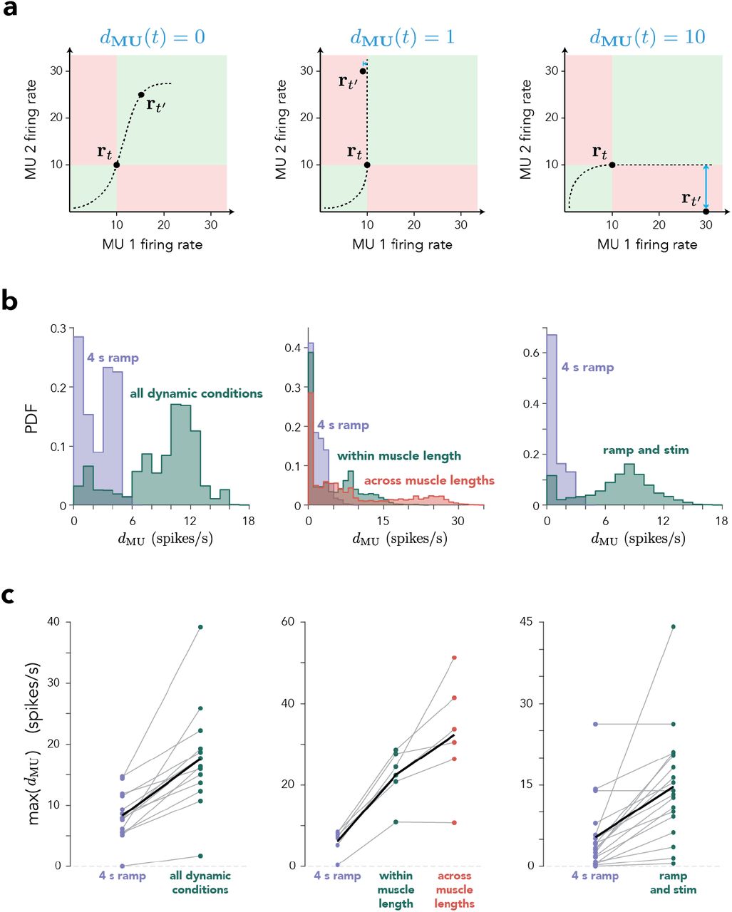
(a) Schematic illustrating, in three situations, the size of the displacement (dMU) for a two-dimensional population state at two times. Left. dMU(t) = 0 because a monotonic manifold can pass through rt and rt′. Center. Any monotonic manifold passing through rt is restricted to the green zone, and thus cannot come closer than 1 spike/s to rt′. Right. A manifold passing through rt can come no closer than 10 spikes/s from rt′. (b) Probability density function (PDF) of dMU(t) for one session for each experiment. dMU(t) was evaluated at every time during the 4 s increasing ramp condition alone, at one muscle length, (purple) or including other conditions. Left. For dynamic experiments, the other conditions were the different force profiles. Center. For muscle-length experiments, the other conditions were different force profiles using the same muscle length (a subset of the force profiles used in the dynamic experiments) or all force profiles across both muscle lengths. Right. For microstimulation experiments, the other conditions involved cortical stimulation (on one of 4-6 electrodes) during static force production at different levels. (c) Maximum displacement (across time) for each condition group shown in b for all sessions. Thin gray lines correspond to different sessions and the thick black line corresponds to the mean across sessions.

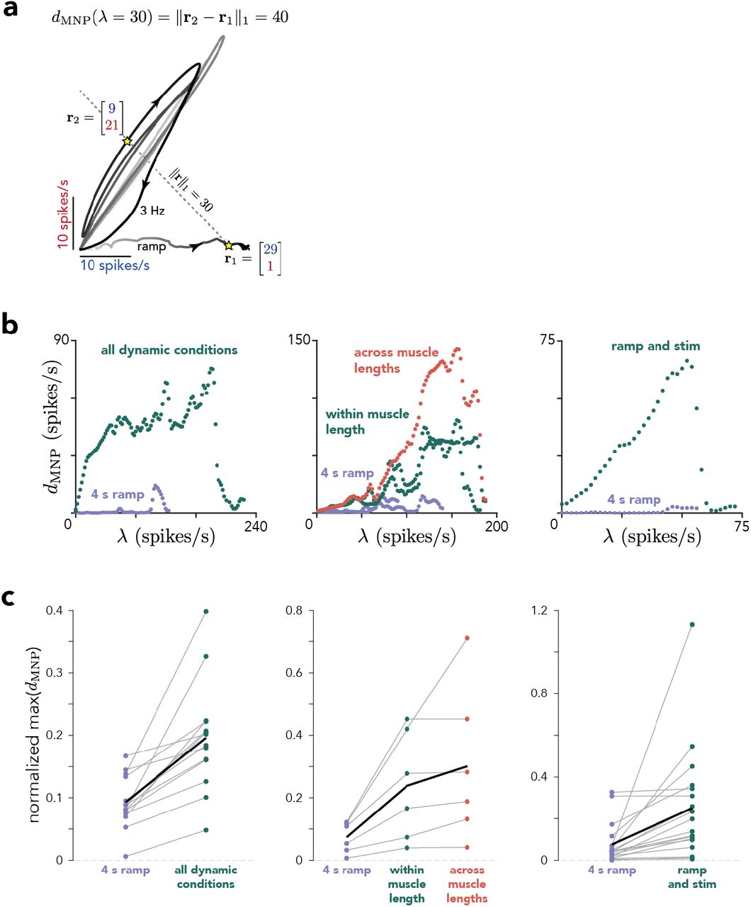
(a) Firing rate of MU309 vs. MU311 during the 4 s increasing ramp and 3 Hz sinusoidal conditions. The line defined by ‖r‖1 = 30 intercepts the activity manifold at several different moments; of those, r1 and r2 are the most separated along the contour line. The MNP dispersion for λ = 30 is the L1-norm of the difference between r1 and r2: 40 spikes/s. (b) Scatter plot of dMNP versus λ for one session for each experiment. dMNP was evaluated at every time during the 4 s increasing ramp condition alone, at one muscle length, (purple) or including other conditions. Left. For dynamic experiments, the other conditions were the different force profiles. Center. For muscle-length experiments, the other conditions were different force profiles using the same muscle length (a subset of the force profiles used in the dynamic experiments) or all force profiles across both muscle lengths. Right. For microstimulation experiments, the other conditions involved cortical stimulation (on one of 4-6 electrodes) during static force production at different levels. (c) Maximum dispersion (across λ) for each condition group shown in b for all sessions. For each session, dMNP(λ) was restricted to the greatest common λ across all condition sets before computing the maximum. Maximum dispersions were normalized by the maximum L1-norm of the MNP response across all times/conditions. Thin gray lines correspond to different sessions and the thick black line corresponds to the mean across sessions.
Latent factor model
The central tenet of rigid control is that all MUs within a pool are controlled by a common drive; different MU activities arise from MU-specific link functions of that drive. We wished to quantitatively evaluate how well this model can account for the joint activity of all simultaneously recorded MUs. Conceptually this approach is simple: the model should be rejected if it fits the data poorly even when granted full expressivity (no constraints other than those inherent to rigid control). Existing models of MU control employ idealized link functions (rectified linear28 or sigmoidal29). While reasonable, those choices limit expressivity. We instead employed a probabilistic latent factor model (Fig. 4a) where the rate of each MU is a function of common drive: ri(t) ~ fi(x(t + τi)). Model fitting used black box variational inference53 to infer x(t) and learn the MU-specific fi and time-lag, τi. fi was unconstrained other than being monotonically increasing.
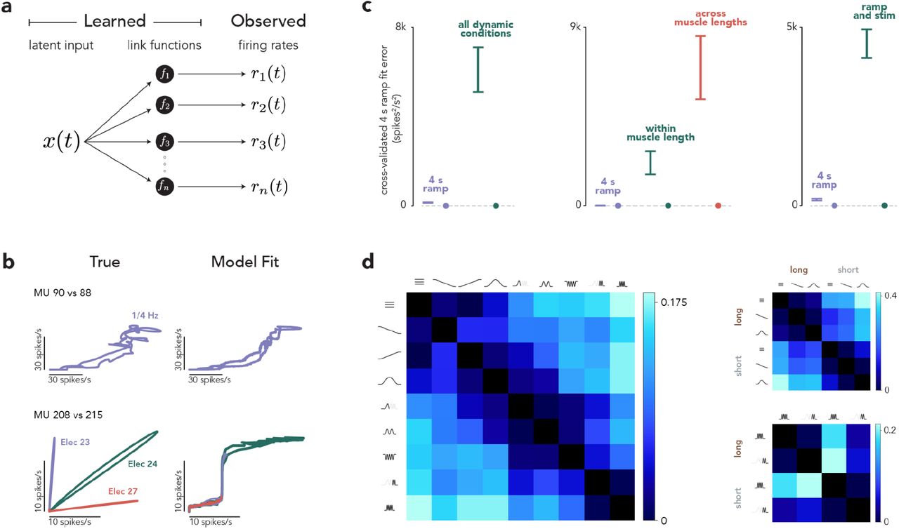
(a) The premise of rigid control is that MU firing rates are fixed ‘link functions’ of a shared, 1-D latent input. If so, it should be possible to infer link functions and a latent that account for the observed rates. We assessed the degree to which this was true, with essentially no constraints other than that link functions be monotonically increasing. (b) Illustration of model fits for simplified situations: the activity of two MUs during a slow ramp (top) or following cortical stimulation on three different electrodes (bottom). (c) Quantification of model performance when accounting for the activity of the full MU population. Cross-validated error was the median (across MUs) dot product of the model residuals (difference between actual and model MU activity) for random splits of trials during the slow-ramp condition alone. Cross-validated error was computed when the model only had to fit the ramp condition, or also had to fit other conditions. Left. For dynamic experiments, the other conditions were the different force profiles. Center. For muscle-length experiments, the other conditions were different force profiles using the same muscle length (a subset of the force profiles used in the dynamic experiments) or all force profiles across both muscle lengths. Right. For microstimulation experiments, the other conditions involved cortical stimulation (on one of 4-6 electrodes) during static force production at different levels. Error bars indicate the mean +/− standard deviation of the cross-validated error across 10 model fits, each using a different random division of the data to compute cross-validated error. Circles indicate fit error when the model was fit to an artificial population response that truly could be described by rigid control, but otherwise closely resembled the empirical population response. (d) Proportion of total MUs that consistently violated the 1-latent model when fit to pairs of conditions. Each entry is the difference between the proportion of consistent violators obtained from the data and the proportion expected by chance. Left: dynamic experiments; right: muscle-length experiments.
The resulting model obeys rigid control but is otherwise highly expressive; it can assume essentially any common drive and set of link functions. Because MUs can have different latencies, it can produce some departures from a monotonic 1D manifold. The model provided good fits during slowly changing forces (Fig. 4b, top). Fit quality suffered in all other situations, including cortical perturbations (Fig. 4b, bottom), because the model could not account for the manifold changing flexibly across situations.
For each session, we fit the activity of all MUs during the 4-second increasing ramp condition, either alone or collectively with other conditions. Error was always computed during the 4-second increasing ramp only. This allowed us to ascertain whether the model’s ability to account for activity during a ‘traditional’ situation was compromised when it had to also account for other situations. Fit error was cross-validated (using random data partitions) and thus should be zero on average for an accurate model. That property was confirmed using an artificial MU population that could be described by one latent factor but was otherwise realistic (accomplished by reconstructing each MU’s response from the first population-level principal component, followed by a rectifying nonlinearity). Fit error was indeed nearly zero for the artificial population (Fig. 4c, filled circles) regardless of how many conditions were fit.
For the empirical data, fit error was nearly zero when the latent variable model was fit only during the 4-second increasing ramp (Fig. 4c, purple). Fits were compromised when the model had to also account for dynamically changing forces, different muscle lengths, or cortical perturbations. This combination of findings explains why the hypothesis of rigid control was appealing (it can describe responses when forces change slowly) while also demonstrating that it fails to describe MU activity once a broader range of behaviors is considered.
We used a complementary approach, focused on single trials, to further explore when the model of rigid control failed. We fit the model to single-trial responses from two conditions at a time. We defined an MU as a ‘consistent violator’ if its activity was overestimated for trials from one condition and underestimated for trials from the other condition, at a rate much higher than chance. Consistent violators indicate that recruitment differs across conditions in a manner inconsistent with rigid control. Consistent violators were relatively rare when two conditions had similar frequency content (Fig. 4d, left, dark entries near diagonal), but became common when conditions had dissimilar frequency content. Additionally, consistent violators became common when comparing across muscle lengths (Fig. 4d, right).
Neural degrees of freedom
If a one-degree-of-freedom (common) drive cannot account for MU activity, how many degrees of freedom must one assume (Fig. 5a)? To identify a lower bound, we fit models with multiple latent factors for two dynamic-experiment sessions (those with the most simultaneously recorded active MUs: 16 and 18). Cross-validated fit error (Fig. 5b) reached zero around 4-6 factors. Thus, describing the activity of the 16-18 MUs required 4-6 degrees of freedom. Because we recorded a minority of MUs (the triceps alone contain a few hundred) from a localized region during a subset of behaviors, there are likely many more degrees of freedom even for a given muscle. Neural control of the arm may thus be quite high-dimensional, with dozens or even hundreds of degrees of freedom once all muscles are considered.

(a) We considered the number of latent inputs that drive MU activity. (b) Cross-validated fit error for models with 1-10 latent factors. Cross-validated error (Fig. 4) was computed across all dynamic-experiment conditions. Error bars indicate the mean +/− standard deviation of that median error across 10 model fits, each using a different random division of the data to compute cross-validated error. (c) We recorded neural activity in M1 using 128-channel Neuropixels probes. (d) Two sets of trial-averaged firing rates were created from even and odd trials. Traces show the projection of the even (green) and odd (purple) population activity onto three principal components (PCs) obtained from the even set. Traces for PCs 1 and 50 were manually offset to aid visual comparison. (e) Reliability of neural latent factors. Two sets of trial-averaged data were obtained from random partitions of single trials. Both data sets were projected onto the principal components (factors) obtained from one set. The reliability of each factor was computed as the correlation between the projection of each data set onto the factor. Traces indicate the mean and 95% confidence intervals (shading) for 25 re-samples of M1 activity (blue) and simulated data with 50 (yellow), 150 (orange), and 500 (red) latent signals.
It is unclear how many of these degrees of freedom are influenced by descending control. Anatomy suggests it could be many. The corticospinal tract alone contains approximately one million axons54, and our perturbation experiments reveal a potential capacity for fine-grained control. A counterargument is that descending commands must be drawn from dimensions occupied by cortical activity, which is typically described as residing in a low-dimensional manifold55–57. In standard tasks, 10-20 latent factors account for most of the variance in M1 activity56–60. Yet the remaining structure, while small, may be meaningful61 given that descending commands appear to be small relative to other signals62.
We reassessed the dimensionality of activity in M1, aided by three features. First, our task involves force profiles spanning a broad frequency range, potentially revealing degrees of freedom not used in other tasks. Second, we considered an unusually large population (881 sulcal neurons) recorded over multiple sessions using the 128-channel version of primate Neuropixels probes. Third, to assess whether a latent factor is meaningful, we focused not on its relative size (i.e., amount of neural variance explained) but on whether it was reliable across trials (Fig. 5d) using a method similar to that of Stringer and colleagues63. When analyzing a subset of neurons, a small but meaningful signal (e.g., one that could be reliably decoded from all neurons) will be corrupted by spiking variability but will still show some nonzero reliability across trials. We defined reliability, for the projection onto a given principal component, as the correlation between held-out data and the data used to identify the principal component (Fig. 5c).
The first two hundred principal components all had reliability greater than zero (Fig. 5e). To put this finding in context, we analyzed artificial datasets that closely matched the real data but had known dimensionality. Even when endowed with 150 latent factors, artificial populations displayed reliability that fell faster than for the data. This is consistent with the empirical population having more than 150 degrees of freedom, an order of magnitude greater than previously considered56–60. For comparison, if M1 simply encoded a force vector, there would be only one degree of freedom; all forces in our experiment were in one direction. Encoding of the force derivative would add only one further degree of freedom. Thus, the M1 population response has enough complexity that it could, in principle, encode a great many outgoing commands beyond force per se. Direct inspection of individual-neuron responses (Fig. S5) supports this view; neurons displayed a great variety of response patterns.

(a) Trial-averaged forces from one session of dynamic experiments (intermediate static force condition is omitted for space). Vertical scale bar indicates 8 N. Horizontal scale bar indicates 1 s. (b-j) Trial-averaged firing rates of M1 neurons with standard error (top) and single-trial spike rasters (bottom). Vertical scale bars indicate 20 spikes/s. Horizontal scale bars indicate 1 s.
Discussion
The hypothesis of rigid control -- a common drive followed by size-based recruitment -- has remained dominant1,25 for three reasons: it describes activity during steady force production4–13, would be optimal in that situation31, and could be implemented via simple mechanisms16,18. It has been argued that truly flexible control would be difficult to implement and that “it is not obvious… that a more flexible, selective system would offer any advantages.18” Yet there has existed evidence, often using indirect means, for at least some degree of flexibility in specific situations45. Our findings argue that flexible MU control is likely a normal aspect of skilled performance in the primate. Recruitment differed anytime two movements involved different force frequencies or muscle lengths.
An appealing hypothesis is that flexibility reflects the goal of optimizing recruitment for each behavior. To test the internal validity of this hypothesis, we employed a normative model of force production by an idealized motor pool where MUs varied in both size and how quickly force peaked and decayed (Supp. Materials). The model employed whatever recruitment strategy maximized accuracy, using knowledge of future changes in force. During slowly changing forces, the model adopted the classic small-to-large recruitment strategy (Fig. S6). During rapidly changing forces, the model adopted different strategies that leveraged heterogeneity in MU temporal force profiles. From this perspective, the size principle emerges as a special case of a broader optimality principle.

Isometric force production was modeled using an idealized motor neuron pool (MNP) containing 5 MUs. MU twitch amplitude varied inversely with contraction time, meaning that small MUs were also slow (see: Supp. Materials for details). The optimal set of MU firing rates for generating a target force profile were numerically derived as the solution that minimized the mean-squared error between the MNP and target forces. (a) Target forces provided to the model (cyan) and MNP force (black) generated using the optimally derived firing rates. (b) Optimal MU firing rates used to generate the MNP force in a. Each color corresponds to a different MU, numbered in ascending order by size (i.e., MU1 was the smallest and slowest). Optimization predicted size-based recruitment for steady force profiles (first two columns), but more flexible recruitment strategies for rapidly changing forces. (c) Firing rates of MU3 (green) plotted against that of MU2 (orange), for each condition shown in b.
Optimal recruitment would require cooperation between spinal and supraspinal mechanisms. Our data support this possibility. Flexibility driven by changes in muscle length presumably depends upon spinally available proprioceptive feedback38. During dynamic movements, some aspects of flexibility reflect future changes in force, which would likely require descending signals. The nature of the interplay between spinal and descending contributions remains unclear, as is the best way to model flexibility. Flexibility could reflect multiple additive drives to the MU pool and/or modulatory inputs that alter input-output relationships52 (i.e., flexible link functions). Both mechanisms could have spinal and/or supraspinal sources.
The hypothesis that descending signals influence MU recruitment has historically been considered implausible, as control might be unmanageably complex unless degrees of freedom are limited3,18. Indeed, descending control has typically been considered to involve muscle synergies64, without even the ability to independently control individual muscles. Consistent with that view, recruitment order is unaltered by supraspinal stimulation in cats27. Recruitment can be altered using biofeedback training in humans65,66, although it is debated whether this ability reflects unexpected flexibility or simply leverages known compartmentalization of multifunctional muscles67,68.
In our view there is little reason to doubt the existence of descending influences on MU recruitment. The corticospinal tract alone contains on the order of a million axons54, including direct connections onto ɑ-motoneurons54,69 from neurons whose diverse responses70 reflect the context in which a force is generated71. Our findings supply three additional reasons to suspect rich descending control. First, during a learned task performed skillfully, recruitment is far more flexible than previously thought. Second, stimulation of neighboring cortical sites can recruit neighboring MUs, disproving the assumption that “the brain cannot selectively activate specific motor units1”. Third, M1 activity has a surprisingly large number of degrees of freedom that could potentially contribute descending commands. Future experiments will need to further explore whether MU recruitment is fully or partially flexible, the level of granularity of descending commands, and how those commands interact with spinal computations.
Author Contributions
M.M.C. conceived the study; N.J.M., M.M.C., and S.M.P. designed experiments; N.J.M. collected and analyzed EMG data sets; N.J.M. and E.M.T. collected neural data sets, supervised by M.M.C. and M.N.S.; J.I.G. trained latent factor models; E.A.A. and N.J.M. analyzed neural data sets; N.J.M. developed the optimal recruitment model, supervised by L.F.A. and M.M.C.; N.J.M. and M.M.C. wrote the paper. All authors contributed to editing.
Methods
Data Acquisition
Subject and task
All protocols were in accord with the National Institutes of Health guidelines and approved by the Columbia University Institutional Animal Care and Use Committee. Subject C was an adult, male macaque monkey (Macaca mulatta) weighing 13 kg.
During experiments, the monkey sat in a primate chair with his head restrained via surgical implant and his right arm loosely restrained. To perform the task, he grasped a handle with his left hand while resting his forearm on a small platform that supported the handle. Once he had achieved a comfortable position, we applied tape around his hand and velcro around his forearm. This ensured consistent placement within and between sessions. The handle controlled a manipulandum, custom made from aluminum (80/20 Inc.) and connected to a ball bearing carriage on a guide rail (McMaster-Carr, PN 9184T52). The carriage was fastened to a load cell (FUTEK, PN FSH01673), which was locked in place. The load cell converted one-dimensional (tensile and compressive) forces to a voltage signal. That voltage was amplified (FUTEK, PN FSH03863) and routed to a Performance real-time target machine (Speedgoat) that executed a Simulink model (MathWorks) to run the task. As the load cell was locked in place, forces were applied to the manipulandum via isometric contractions.
The monkey controlled a ‘Pac-Man’ icon, displayed on an LCD monitor (Asus PN PG258Q, 240 Hz refresh, 1920 x 1080 pixels) using Psychophysics Toolbox 3.0. Pac-Man’s horizontal position was fixed on the left hand side of the screen. Vertical position was directly proportional to the force registered by the load cell. For 0 Newtons applied force, Pac-Man was positioned at the bottom of the screen; for the calibrated maximum requested force for the session, Pac-Man was positioned at the top of the screen. Maximum requested forces (see: Experimental Procedures, below) were titrated to be comfortable for the monkey to perform across multiple trials and to activate multiple MUs, but not so many that rendered EMG signals unsortable. On each trial, a series of dots scrolled leftwards on screen at a constant speed (1344 pixels/s). The monkey modulated Pac-Man’s position to intercept the dots, for which he received juice reward. Thus, the shape of the scrolling dot path was the temporal force profile the monkey needed to apply to the handle to obtain reward. We trained the monkey to generate static, step, ramp, and sinusoidal forces over a range of amplitudes and frequencies. We define a ‘condition’ as a particular target force profile (e.g., a 2 Hz sinusoid) that was presented on many ‘trials’, each a repetition of the same profile. Each condition included a ‘lead-in’ and ‘lead-out’ period: a one-second static profile appended to the beginning and end of the target profile, which facilitated trial alignment and averaging (see below). Trials lasted 2.25-6 seconds, depending on the particular force profile. Juice was given throughout the trial so long as Pac-Man successfully intercepted the dots, with a large ‘bonus’ reward given at the end of the trial.
The reward schedule was designed to be encouraging; greater accuracy resulted in more frequent rewards (every few dots) and a larger bonus at the end of the trial. To prevent discouraging failures, we also tolerated small errors in the phase of the response at high frequencies. For example, if the target profile was a 3 Hz sinusoid, it was considered acceptable if the monkey generated a sinusoid of the correct amplitude and frequency but that led the target by 100 ms. To enact this tolerance, the target dots sped up or slowed down to match his phase. The magnitude of this phase correction scaled with the target frequency and was capped at +/− 3 pixels/frame. To discourage inappropriate strategies (e.g., moving randomly, or holding in the middle with the goal if intercepting some dots) a trial was aborted if too many dots were missed (the criterion number was tailored for each condition).
Surgical procedures
After task performance stabilized at a high level, we performed a sterile surgery to implant a cylindrical chamber (Crist Instrument Co., 19 mm inner diameter) that provided access to M1. Guided by structural magnetic resonance imaging scans taken prior to surgery, we positioned the chamber surface-normal to the skull, centered over the central sulcus. We covered the skull within the cylinder with a thin layer of dental acrylic. Small (3.5 mm), hand-drilled burr holes through the acrylic provided the entry point for electrodes.
Intracortical recordings and microstimulation
Neural activity was recorded with Neuropixels probes. Each probe contained 128 channels (two columns of 64 sites). Probes were lowered into position with a motorized microdrive (Narishige). Recordings were made at depths ranging from 5.6 - 12.1 mm relative to the surface of the dura. Raw neural signals were digitized at 30 kHz and saved with a 128-channel neural signal processor (Blackrock Microsystems, Cerebus).
Intracortical electrical stimulation (20 biphasic pulses, 333 Hz, 400 μs phase durations, 200 μs interphase) was delivered through linear arrays (Plexon Inc., S-Probes) using a neurostimulator (Blackrock Microsystems, Cerestim R96). Each probe contained 32 electrode sites with 100 μm separation between them. Probes were positioned with a motorized microdrive (Narishige). We estimated the target depth by recording neural activity prior to stimulation sessions. Each stimulation experiment began with an initial mapping, used to select 4-6 electrode sites to be used in the experiments. That mapping allowed us to estimate the muscles activated from each site, and the associated thresholds. Thresholds were determined based on visual observation and were typically low (10-50 μA), but occasionally quite high (100-150+ μA) depending on depth. Across all 32 electrodes, microstimulation induced twitches of proximal and distal muscles of the upper arm, ranging from the deltoid to the forearm. Rarely did an electrode site fail to elicit any response, but many responses involved multiple muscles or gross movements of the shoulder that were difficult to attribute to a specific muscle. Yet some sites produced more localized responses, prominent only within a single muscle head. Sometimes a narrow (few mm2) region within the head of one muscle would reliably and visibly pulse following stimulation. Because penetration locations were guided by recordings and stimulation on previous days, such effects often involved the muscles central to performance of the task: the deltoid and triceps. In such cases, we selected 4-6 sites that produced responses in one of these muscles, and targeted that muscle with EMG recordings. EMG recordings were always targeted to a localized region of one muscle head (see below). In cases where stimulation appeared to activate only part of one muscle head, EMG recordings targeted that localized region.
EMG recordings
Intramuscular EMG activity was recorded acutely using paired hook-wire electrodes (Natus Neurology, PN 019-475400). Electrodes were inserted ~1 cm into the muscle belly using 30 mm x 27 G needles. Needles were promptly removed and only the wires remained in the muscle during recording. Wires were thin (50 um diameter) and flexible and their presence in the muscle is typically not felt after insertion, allowing the task to be performed normally. Wires were removed at the end of the session.
We employed several modifications to facilitate isolation of MU spikes. As originally manufactured, two wires protruded 2 mm and 5 mm from the end of each needle (thus ending 3 mm apart) with each wire insulated up to a 2 mm exposed end. We found that spike sorting benefited from including 4 wires per needle (i.e., combining two pairs in a single needle), with each pair having a differently modified geometry. Modifying each pair differently meant that they tended to be optimized for recording different MUs1; one MU might be more prominent on one pair and the other on another pair. Electrodes were thus modified as follows. The stripped ends of one pair were trimmed to 1 mm, with 1 mm of one wire and 8 mm of the second wire protruding from the needle’s end. The stripped ends of the second pair were trimmed to 0.5 mm, with 3.25 mm of one wire and 5.25 mm of the second wire protruding. Electrodes were hand fabricated using a microscope (Zeiss), digital calipers, precision tweezers and knives. During experiments, EMG signals were recorded differentially from each pair of wires with the same length of stripped insulation; each insertion thus provided two active recording channels. Four insertions (closely spaced so that MUs were often recorded across many pairs) were employed, yielding eight total pairs. The above approach was used for both the dynamic and muscle-length experiments, where a challenge was that normal behavior was driven by many MUs, resulting in spikes that could overlap in time. This was less of a concern during the microstimulation experiments. Stimulation-induced responses were typically fairly sparse near threshold (a central finding of our study is that cortical stimulation can induce quite selective MU recruitment). Thus, microstimulation experiments employed one electrode pair per insertion, with minimal modification (exposed ends shorted to 1 mm).
Raw voltages were amplified and analog filtered (band-pass 10 Hz - 10 kHz) with ISO-DAM 8A modules (World Precision Instruments), then digitized at 30 kHz with a neural signal processor (Blackrock Microsystems, Cerebus). EMG signals were digitally band-pass filtered online (50 Hz - 5 kHz) and saved.
Experimental procedures
Cortical recordings were performed exclusively during one set of experiments (‘dynamic’, defined below), whereas EMG recordings were conducted across three sets of experiments (dynamic, ‘muscle length’, and microstimulation). In a given session, the eight EMG electrode pairs were inserted within a small (typically ~2 cm2) region of a single muscle head. This focus aided sorting by ensuring that a given MU spike typically appeared, with different waveforms, on multiple channels. This focus also ensured that any response heterogeneity was due to differential recruitment among neighboring MUs.
In dynamic experiments, the monkey generated a diverse set of target force profiles. The manipulandum was positioned so that the angle of shoulder flexion was 25° and the angle of elbow flexion was 90°. Maximal requested force was 16 Newtons. We employed twelve conditions (Supp Fig. 1) presented interleaved in pseudo-random order: a random order was chosen, all conditions were performed, then a new random order was chosen. Three conditions employed static target forces: 33%, 66% and 100% of maximal force. Four conditions employed ramps: increasing or decreasing across the full force range, either fast (lasting 250 ms) or slow (lasting 4 s). Four conditions involved sinusoids at 0.25, 1, 2, and 3 Hz. The final condition was a 0-3 Hz chirp. The amplitude of all sinusoidal and chirp forces was 75% of maximal force, except for the 0.25 Hz sinusoid, which was 100% of maximal force. Recordings in dynamic experiments were made from the deltoid (typically the anterior head and some from the lateral head) and the triceps (lateral head).
In muscle-length experiments, the monkey generated force profiles with his deltoid at a long or short length (relative to the neural position used in the dynamic experiments). The manipulandum was positioned so that the angle of shoulder flexion was 15° (long) or 50° (short), while maintaining an angle of elbow flexion of 90°. Maximal requested forces were 18 N (long) and 14 N (short). Different maximal forces were employed as it appeared more effortful to generate forces in the shortened position. To ensure enough trials per condition, we employed only a subset of the force profiles used in the dynamics experiments. These were 2 static forces (50% and 100% of maximal force), the slow increasing ramp, both increasing and decreasing fast ramps, all four sinusoids and the chirp. These were presented interleaved in pseudorandom order for multiple trials (~30 per condition) for the lengthened position (15°) before changing to the shortened position (50°). In most experiments we were able to revert to the lengthened position (15°) at the end of the session, and verify that MU recruitment returned to the originally observed pattern. Recordings in muscle-length experiments were made from the deltoid (anterior head).
Microstimulation experiments employed recordings from the lateral deltoid and lateral triceps. Both these muscles exhibited strong task-modulated activity, as documented in the dynamic and muscle-length experiments. We also included recordings from the sternal pectoralis major, which showed only modest task-modulated activity, as we found cortical sites that reliably activated it. The manipulandum was positioned so that the angle of shoulder flexion was 25° and the angle of elbow flexion was 90° (as in dynamic experiments). Maximal force was typically set to 16 N, but was increased to 24 N and 28 N for two sessions each in an effort to evoke greater muscle activation. Microstimulation experiments employed a limited set of force profiles: four static forces (0, 25%, 50% and 100%), and the slow (4 s) increasing ramp. The ramp was included to document the natural recruitment pattern during slowly changing forces. Microstimulation was delivered once per trial during the static forces, at a randomized time (1000-1500 ms relative to when the first dot reached Pac-Man). Because stimulation evoked activity in muscles used to perform the task, it sometimes caused small but detectable changes in force applied to the handle. However, these were so small that they did not impact the monkey’s ability to perform the task and appeared to go largely unnoticed. These experiments involved a total of 17-25 conditions: the ramp condition (with no stimulation) plus the four static forces for the 4-6 chosen electrode sites. These were presented interleaved in pseudorandom order.
Data Processing
Signal processing and spike sorting
Cortical voltage signals were spike sorted using KiloSort 2.02. A total of 881 neurons were isolated across 15 sessions.
EMG signals were digitally filtered offline using a second-order 500 Hz high-pass Butterworth. Any low SNR or dead EMG channels were omitted from analyses. Motor unit (MU) spike times were extracted using a custom semi-automated algorithm. As with standard spike-sorting algorithms used for neural data, individual MU spikes were identified based on their match to a template: a canonical time-varying voltage across all simultaneously recorded channels (example templates are shown in Fig. 1d, bottom left). A distinctive feature of intramuscular records (compared to neural recordings) is that they have very high signal-to-noise (peak-to-peak voltages on the order of mV, rather than uV, and there is negligible thermal noise) but it is common for more than one MU to spike simultaneously, yielding a superposition of waveforms. This is relatively rare at low forces but can become common as forces increase. Our algorithm was thus tailored to detect not only voltages that corresponded to single MU spikes, but also those that resulted from the superposition of multiple spikes. Detection of superposition was greatly aided by the multi-channel recordings; different units were prominent on different channels. Further details are provided in the Supplementary Methods.
Trial alignment and averaging
Single-trial spike rasters, for a given neuron or MU, were converted into a firing rate via convolution with a 25 ms Gaussian kernel. One analysis (Fig. 4d) focused on single-trial responses, but most employed trial-averaging to identify a reliable average firing rate. To do so, trials for a given condition were aligned temporally and the average firing rate, at each time, was computed across trials. Stimulation trials were simply aligned to stimulation onset. For all other conditions, each trial was aligned on the moment the target force profile ‘began’ (when the target force profile, specified by the dots, reached Pac-Man). This alignment brought the actual (generated) force profile closely into register across trials. However, because the actual force profile could sometimes slightly lead or lag the target force profile, some modest across-trial variability remained. Thus, for all trials with changing forces, we realigned each trial (by shifting it slightly in time) to minimize the mean squared error between the actual force and the target force profile. This ensured that trials were well-aligned in terms of the actual generated forces (the most relevant quantity for analyses of MU activity). Trials were excluded from analysis if they could not be well aligned despite searching over shifts from −200 to 200 ms.
Data Analysis
Quantifying motor unit flexibility
We developed two analyses that quantified MU-recruitment flexibility without directly fitting a model (model-based quantification is described below). These two analyses were used to produce the results in Figures S2 and S3, respectively. Both methods leverage the definition of rigid control to detect patterns of activity that are inconsistent with rigid control even under the most generous of assumptions.
Let rt = [r1, t r2, t ··· rn, t]⊤ denote the population state at time t, where ri, t denotes the firing rate of the ith MU. If rt traverses a 1-D monotonic manifold, then as the firing rate of one MU increases, the firing rate of all others should either increase or remain the same. More generally, the change in firing rates from t to t′ should either be nonnegative or nonpositive for all MUs. If the changes in firing rate were all nonnegative with some increases, then we could infer that a common input drive increased from t to t′. Equivalently, we could conclude that the common drive decreased from t′ to t. Both these cases (all nonnegative or all nonpositive) are consistent with rigid control because there exists some 1-D monotonic manifold that contains the data at both t′ and t.
On the other hand, departures from a 1-D monotonic manifold can be inferred as moments when the firing rates of one or more MUs increase as others’ decrease. Both our analyses seek to quantify the magnitude of such departures while being very conservative. Specifically, the size of a departure was always measured as the smallest possible discrepancy from a 1-D manifold, based on all possible 1-D manifolds. To illustrate the importance of this conservative approach, consider a situation where the firing rate of MU1 increases considerably while MU2’s rate decreases slightly from t to t′. This scenario would be inconsistent with activity being modulated solely by a common input, yet it would be impossible to know which MU reflected an additional or separate input. Perhaps common drive decreased slightly (explaining the slight decrease in MU2’s rate) but MU1 received an additional large, private excitatory/inhibitory input. This would indicate a large departure from rigid control. Yet another possibility is that common drive increased considerably (explaining the large increase in MU1’s rate) and that MU2’s rate failed to rise because it was already near maximal firing rate. This would not explain why MU2’s rate went down, but if that decrease was small it could conceivably be due to a very modest departure from idealized rigid control. Thus, to be conservative, one should quantify this situation as only a slight deviation from the predictions of rigid control. Both methods described below were designed to do so; when MU activities were anticorrelated, we identified the largest increase and decrease in firing rates, then reported the change that was smaller in magnitude.
For the first analysis, we computed the largest nonnegative change in firing rates from t to t′ for a population of n MUs as

If a 1-D monotonic manifold can be drawn through rt and rt′, then either Δr+ (t, t′) or Δr+ (t′, t) will be zero. Otherwise, Δr+ (t, t′) will capture the largest increase (across MUs) in rate from t to t′ while Δr+ (t′, t) will capture the largest decrease. Thus, we computed departures from a monotonic manifold at the level of an individual MU as

As examples, consider a population of two MUs with rt = [10, 10] and rt′ = [15, 25]. These states would be consistent with an increase in common drive from t to t′, so D(t, t′) (Supp Fig. S2a, left). Conversely, rt = [10, 10] and rt′ = [9, 30] (center) suggests a violation of rigid control, but that violation might be small; one can draw a manifold that passes through [10, 10] and comes within 1 spike/s of [9, 30]. In this case, D(t,t′) = 1. Finally, rt = [10, 10] and rt′ = [0, 30] (right) argue for a sizable violation; [0, 30] is at least 10 spikes/s distant from any monotonic manifold passing through [10, 10], so D(t,t′) = 10.
It is worth emphasizing that (eq. 2) can readily be computed for a population with more than two MUs, but the analysis ultimately reduces to a comparison of two MUs: one whose firing rate increased the most and the other whose firing rate decreased the most across a pair of time points.
To extend our analysis to multiple time points, we computed the ‘MU displacement’ as
 where t′ indexes over all other times and conditions, and τ and τ′ are time lags. The inclusion of time lags ensures that departures from a monotonic manifold cannot simply be attributed to modest differences in response latencies across MUs. In our analyses, we optimized over τ, τ′ ∈ [−25, 25] ms. dMU is exceedingly conservative; it makes no assumptions regarding the manifold other than that it is monotonic, and identifies only those violations that are apparent when comparing just two times.
An advantage of the dMU metric is interpretational simplicity; it identifies pairs of times where the joint activity of two MUs cannot lie on a single 1-D monotonic manifold. A disadvantage is that it does not also capture the degree to which multiple other MUs might also have activity inconsistent with a 1-D monotonic manifold. To do so, we employed a second metric that quantifies MU-recruitment flexibility at the population level. Under the assumptions of rigid control, the magnitude of common drive determines the population state and therefore the summed activity of all MUs or, equivalently, its L1-norm, ‖r‖1. Increases and decreases in common drive correspond, in a one-to-one manner, to increases and decreases in ‖r‖1. Violations of rigid control can thus be inferred if a particular norm value, λ, is associated with different population states. Geometrically, this corresponds to the population activity manifold intersecting the hyperplane defined by ‖r‖1 = λ at multiple locations.
We thus defined the motor neuron pool (MNP) dispersion as
 where τ1, τ2 are time lag vectors, of the same dimensionality as r, and ϵ is a small constant. Conceptually, the dispersion identifies the pair of time points when the population states are the most dissimilar, while having norms within ϵ of λ. As when computing dMU(t), we minimized dMNP(λ) over time lags so as to only consider dispersions that could not be simply attributed to latency differences across MUs. For our analyses, we set ϵ = 1 and optimized over τ1, τ2 ∈ [−25, 25] ms.
Latent factor model
We developed a probabilistic latent variable model of MU activity. Let xt be the unknown latent variables at time t, which are shared between all MUs. We can fit this model with one latent (Fig. 4; xt can be a single value) or multiple latents (Fig. 5). Let yi,t be the activity of the ith MU at time t, given by
 where fi denotes the link function for the ith MU and τi denotes the lag between its response and the shared latent variables. We constrained τi ∈ [−25, 25] ms. To identify flexible, monotonically increasing link functions with nonnegative outputs, we parameterized fi as a rectified monotonic neural network. More precisely, we fit each fi using a two-layer feedforward neural network in which the weights were constrained to be positive. The positivity constraint was achieved by letting each weight w = ln(1 + eu), where the values of u were fit within the model. During model training, the output of the neural network was passed through a ‘leaky rectified linear unit’ (i.e., so that the output was never exactly zero). After training was completed, we used standard rectification on the output.
When predicting held-out data, we encouraged temporal smoothness in the latent space to improve generalization performance by letting  , where smaller values of σ encouraged greater smoothness. We set σ to 0.01 for our analyses.
To infer the most likely distribution of latent variables given the data (i.e., the model posterior, p(x|y)), and to learn the link functions and other parameters, we used variational inference with a mean-field approximation for the posterior approximation. As an inference method, we used black-box variational inference3, which performs gradient descent to maximize the model’s evidence lower bound. We iterated between (1) optimizing the posterior and all parameters while holding response lags fixed and (2) optimizing the response lags. Post model-fitting, when predicting MU activity, we used the mean of the posterior distribution as the latent input at each time.
Prior to fitting the model, the firing rate of each MU was normalized by its maximum response across conditions. Normalization did not alter the ability of the model to fit the data, but simply encouraged the model to fit all MUs, rather than just the high-rate units. Additionally, the likelihood of each time point was weighted by the duration of the experimental condition, so that each condition mattered equally within the model regardless of duration. When fitting to single trials, we also weighted each condition by its trial count, again so that each condition had equal importance. All model fits were done within individual sessions.
Residual error plots
To compute the cross-validated model residuals, we first randomly split the single-trial firing rates for each MU into halves, and computed the trial-average responses for each half: yi,1 and yi,2. We then fit the latent variable model to each half, which yielded a pair of predicted responses,  and
and  . The cross-validated model residuals were calculated as the dot product between the residual errors of each half:
  . We computed the median cross-validated residuals across all MUs and sessions for a given partitioning of the data. The above steps were then repeated for 10 different random splits of trials and we reported the mean +/− standard error of the median error across re-partitions and fits.
As a control (Fig. 4), we modified the data so that a single latent variable could fully account for all responses. To do so, we reconstructed the firing rates using only the first principle component of the trial average firing rates. For example, if w is the n × 1 loading vector for the first principal component, then Y1, the ct × n matrix of responses for one partitioning of the data, was reconstructed as [Y1ww⊤]+, where the rectification ensures that all firing rates are non-negative. Using these reconstructed firing rates, we performed the same residual error analysis. Because of the rectification, the modified data are not one-dimensional in the linear sense (there would be multiple principal components with non-zero variance). Yet because the data will lie on a one-dimensional monotonic manifold, cross-validated error should be near zero when fitting the model, which is indeed what we observed.
Consistency plots
We fit the model to the activity of single trials. We aimed to determine whether, when fit to two conditions, the model consistently overestimated the true firing rates in one condition and underestimated the firing rates in the other condition. To do so, we calculated the mean model error across time on every trial for each condition. Let E(1, tr) and E(2, tr) denote the mean errors for a particular MU, pair of conditions (indexed by 1 and 2), and trial tr. We calculated the consistency for the MU and conditions as
 where
where
 n is the total number of trials across both conditions, and 1A is the indicator function (1 if A is true; 0 otherwise). Eq. (6) determines the fraction of times one condition had negative errors and the other had positive errors, while accounting for trials with no error. Prior to performing this consistency calculation, we set all E(j, tr) with absolute value less than 0.01 to 0, so that the sign of negligible errors was not considered. We also removed E(1, tr) or E(2, tr) in which the MU had zero actual and predicted activity, because it was impossible for the predicted activity to undershoot the true activity in this setting.
We calculated the fraction of MUs that had C > 0.8 and an average error of at least 0.01 across trials (to ensure that outlier trials did not lead to false positives of consistent errors). We excluded MUs who had zero activity in > 80% of trials in the two conditions being analyzed. Consequently, the number of MUs included in the analysis) varied for each pair of conditions.
To calculate a chance-level baseline (Fig. S4), for each MU, we calculated the probability that greater than 80% of the included trials would have a positive or negative error, assuming that each trial has an independent 50/50 chance of being positive or negative. More precisely, let F(k; n, p) be the cumulative density function of a binomial distribution of having k successes in n Bernoulli events, each event with probability p of being a success. We calculate Pi = 2(1 − F(ceil[0.8ni]; ni, 0.5)), where ni is the number of total trials included for MU i and ceil[] gets the next integer. The total expected fraction of MUs with C > 0.8 by chance is thus  .
.
Cross-validated reliability dimensionality estimate
To estimate the dimensionality of M1, we randomly split the single-trial firing rates for each neuron into two groups and averaged over trials within each group. Let Y1 and Y2 denote the CT × N matrices of trial-averaged responses for each partition (CT condition-times and N neurons). Let wi (an N × 1 vector) denote the ith principal component (PC) of Y1. The reliability of PC i was computed as the correlation between Y1wi and Y2wi. We repeated this process for 25 re-partitions over trials to obtain confidence intervals. Our method is inspired by Churchland et al.4 and conceptually similar to but distinct from the cross-validated PCA analysis of Stringer et al., which estimates the stimulus-related (‘signal’) neural variance based on spontaneous activity across many neurons on single trials5.
To create simulated data sets with dimensionality k, we computed  , where Y is the matrix of M1 firing rates averaged over all trials, and Qk denotes the first k columns of a random orthonormal matrix. Simulated single-trial spikes were generated for each neuron using an inhomogeneous Poisson process with rate given by the corresponding column of Yk. Simulated spikes were smoothed using a 25 ms Gaussian kernel, and the cross-validated reliability metric applied as described above.
Acknowledgements
We thank Y. Pavlova for fantastic animal care. This work was supported by the Grossman Charitable Trust, Simons Foundation (M.M.C., J.P.C., and L.F.A.), McKnight Foundation (M.M.C. and J.P.C.), NIH Director’s DP2 NS083037 (M.M.C.), NIH CRCNS R01NS100066 (M.M.C. and J.P.C.), NIH 1U19NS104649 (M.M.C., L.F.A., and J.P.C.), NIH F31 NS110201 (N.J.M.), NIH K99 NS119787 (J.I.G.), NSF GRFP (N.J.M.), NSF NeuroNex (J.I.G. and L.F.A.), Kavli Foundation (M.M.C. and L.F.A.), Howard Hughes Medical Institute (M.N.S.), and Gatsby Charitable Foundation (J.I.G., L.F.A., and J.P.C.).


