

Abstract
Natural selection acts on phenotypes constructed over development, which raises the question of how development affects evolution. Classic evolutionary theory indicates that development affects evolution by modulating the genetic covariation upon which selection acts, thus affecting genetic constraints. However, whether genetic constraints are relative, thus diverting adaptation from the direction of steepest fitness ascent, or absolute, thus blocking adaptation in certain directions, remains uncertain. This limits understanding of long-term evolution of developmentally constructed phenotypes. Here we formulate a general tractable mathematical framework that integrates age progression, explicit development (i.e., the construction of the phenotype across life subject to developmental constraints), and evolutionary dynamics, thus describing the evolutionary developmental (evo-devo) dynamics. The framework yields simple equations that can be arranged in a layered structure that we call the evo-devo process, whereby five elementary components generate all equations including those describing genetic covariation and the evo-devo dynamics. The framework recovers evolutionary dynamic equations in gradient form and describes the evolution of genetic covariation from the evolution of gene expression, phenotype, environment, and mutational covariation. This shows that genetic and phenotypic evolution must be followed simultaneously to yield a well-defined description of long-term phenotypic evolution in gradient form, such that evolution described as the climbing of a fitness landscape occurs in geno-phenotype space. Genetic constraints in geno-phenotype space are necessarily absolute because the degrees of freedom of genetic covariation are necessarily limited by genetic space. Thus, the long-term evolutionary dynamics of developed phenotypes is strongly non-standard: (1) evolutionary equilibria are either absent or infinite in number and depend on genetic covariation and hence on development; (2) developmental constraints determine the admissible evolutionary path and hence which evolutionary equilibria are admissible; and (3) evolutionary outcomes occur at admissible evolutionary equilibria, which do not generally occur at fitness landscape peaks in geno-phenotype space, but at peaks in the admissible evolutionary path where “total genetic selection” vanishes if exogenous plastic response vanishes and mutational variation exists in all directions of gene-expression space. Development thus modulates necessarily absolute genetic constraints, and hence it affects evolutionary equilibria, the admissible evolutionary path, and which equilibria are admissible. Our framework provides an alternative method to dynamic optimization (i.e., dynamic programming or optimal control) to identify evolutionary outcomes in models with developmentally dynamic traits. These results show that development has major evolutionary effects.
1. Introduction
Natural selection screens phenotypes produced by development, defined as “the process by which genotypes are transformed into phenotypes” (Wolf et al., 2001). Thus, a fundamental evolutionary problem concerns how development affects evolution. Interest in this problem is long-standing (Baldwin 1896, Waddington 1959 p. 399, and Gould and Lewontin 1979) and has steadily increased in recent decades. It has been proposed that developmental constraints (Gould and Lewontin, 1979; Maynard Smith et al., 1985; Brakefield, 2006; Klingenberg, 2010), causal feedbacks among gene expression, phenotype, and environment occurring through development (Lewontin, 1983; Rice, 2011; Hansen, 2013; Laland et al., 2015), and some development-mediated factors (Laland et al., 2014, 2015), namely plasticity (West-Eberhard, 2003), niche construction (Odling-Smee et al., 1996, 2003), extra-genetic inheritance (Baldwin, 1896; Cavalli-Sforza and Feldman, 1981; Boyd and Richerson, 1985; Bonduriansky and Day, 2018), and developmental bias (Arthur, 2004), may all have important evolutionary roles. Understanding how development — including these elements acting individually and together — affects the evolutionary process remains an outstanding challenge (Baldwin, 1896; Waddington, 1959; Müller, 2007; Pigliucci, 2007; Laland et al., 2014, 2015; Galis et al., 2018).
Classic evolutionary theory indicates that development affects evolution by modulating the genetic covariation upon which selection acts. This can be seen as follows. In quantitative genetics, an individual’s i-th trait value xi is written as  , where the overbar denotes population average, yj is the individual’s gene content at the j-th locus, αij is the partial regression coefficient of the i-th trait deviation from the average on the deviation from the average of the j-th locus content, and ei is the residual error (Fisher, 1918; Crow and Kimura, 1970; Falconer and Mackay, 1996; Lynch and Walsh, 1998; Walsh and Lynch, 2018). The quantity αij is Fisher’s additive effect of allelic substitution (his α; see Eq. I of Fisher 1918 and p. 72 of Lynch and Walsh 1998) and is the linear description of development, namely of how genotypes are transformed into phenotypes. In matrix notation, the vector of an individual’s trait values is
  , where the matrix α corresponds to what Wagner (1984) calls the developmental matrix (his B). The breeding value of the multivariate phenotype x is defined as
  , which does not consider the error term that includes non-linear effects of genes on phenotype. Breeding value thus depends on development via the developmental matrix α. The Lande (1979) equation describes the evolutionary change due to selection in the mean multivariate phenotype
  as
as  , where the additive genetic covariance matrix is G ≡ cov[ax, ax] = αcov[y, y]α⊤ (e.g., Wagner 1984), absolute fitness is W, and the selection gradient is
  , which points in the direction of steepest increase in mean fitness. An important feature of the Lande equation is that it is in gradient form, so the equation shows that, within the assumptions made, phenotypic evolution by natural selection proceeds as the climbing of a fitness landscape, as first shown by Wright (1937) for frequency change of two alleles in a single locus. Moreover, the Lande equation shows that additive genetic covariation, described by G, may divert evolutionary change from the direction of steepest fitness ascent, and may prevent evolutionary change in some directions if genetic variation in those directions is absent (in which case G is singular). Since additive genetic covariation depends on development via the developmental matrix a, the Lande equation shows that development affects evolution by modulating genetic covariation via α (Charlesworth et al., 1982; Cheverud, 1984; Maynard Smith et al., 1985).
However, this mathematical description might have limited further insight into the evolutionary effects of development, particularly because it lacks two key pieces of information. First, the above description yields a limited understanding of the form of the developmental matrix α. The definition of α as a matrix of regression coefficients does not make available a developmentally explicit nor evolutionarily dynamic understanding of α, which hinders understanding of how development affects evolution. Although the developmental matrix α has been modelled (Pavlicev and Hansen, 2011) or analysed as unknowable (Martin, 2014), there is a lack of a general theory with an explicit description of the developmental process to unveil the general structure of the developmental matrix α.
Second, the description in the second paragraph above gives a very short-term account of the evolutionary process. The Lande equation in the second paragraph strictly describes the evolution of mean traits  but not of mean gene content
  , that is, it does not describe change in allele frequency; yet, since α is a matrix of regression coefficients calculated for the current population, α depends on the current state of the population including allele frequency
  . Thus, the Lande equation above describes the dynamics of some traits
  as an implicit function of traits
  whose dynamics are not described. The equation thus contains fewer dynamic equations (as many as there are traits in
  ) than dynamic variables (as many as there are traits
  and loci
  ), so it is underdetermined. Consequently, the Lande equation strictly admits an infinite number of evolutionary trajectories for a given initial condition. Technically, the evolutionary trajectory is ill-defined by the Lande’s system (we note that this harsh-sounding term does not mean that the Lande equation is wrong; a common term in this context is “dynamically insufficient” but ill-definition is an older and widespread mathematical notion). The standard approach to this ill-definition is to assume Fisher’s infinitesimal model, whereby there is an infinite number of loci such that allele frequency change per locus per generation is negligible (Bulmer, 1971, 1980; Turelli and Barton, 1994; Barton et al., 2017; Hill, 2017). Thus, the Lande equation is said to describe short-term evolution, during which there is negligible allele frequency change per locus (Walsh and Lynch, 2018, pp. 504 and 879). The Lande equation is then supplemented by the Bulmer (1980) equation (Lande and Arnold, 1983, Eq. 12) which describes the dynamics of G primarily due to change in linkage disequilibrium under the assumption of negligible allele frequency change, thus still to describe short-term evolution (Walsh and Lynch, 2018, p. 553). Typically, the G matrix is assumed to have reached an equilibrium in such short-term dynamics or to remain constant although this has often been shown not to hold theoretically (Turelli, 1988) and empirically (Bjorklund et al., 2013). An alternative to the ill-definition of the evolutionary trajectory described by the classic Lande’s system would be to consider the vector of gene content y to be a subvector of the vector of trait values x (Barfield et al., 2011), although such vector x does not admit the normality assumption of the Lande equation and doing so does not yield a description of linkage disequilibrium dynamics. Indeed, there appears to be no formal derivation of such extended Lande’s system that makes explicit the properties of its associated G-matrix and the dependence of such matrix on development. Overall, understanding how development affects evolution using the classic Lande equation might have been hindered by a lack of a general mechanistic understanding of the developmental matrix α and by the generally ill-defined evolutionary trajectory entailed by the classic Lande’s system.
Nevertheless, there has been progress on general mathematical aspects of how development affects evolution on various fronts. Both the classic Lande equation (Lande, 1979) and the classic canonical equation of adaptive dynamics (Dieckmann and Law, 1996) describe the evolutionary dynamics of a multivariate trait in gradient form without an explicit account of development, by considering no explicit age progression or developmental (i.e., dynamic) constraints (there is also an analogous equation for allele frequency change for multiple alleles in a single locus, first incorrectly presented by Wright, 1937 but later corrected by Edwards, 2000 and presented in Lande’s form by Walsh and Lynch, 2018, Eq. 5.12a). Various research lines have extended these equations to incorporate different aspects of development. First, one line considers explicit age progression by implementing age structure, which allows individuals of different ages to coexist and to have age-specific survival and fertility rates. Thus, evolutionary dynamic equations in gradient form for age-structured populations have been derived under quantitative genetics assumptions (Lande, 1982), population genetics assumptions (Charlesworth, 1993, 1994), and adaptive dynamics assumptions (Durinx et al., 2008). An important feature of age-structured models is that the forces of selection decline with age due to demography, in particular due to mortality and fewer remaining reproductive events as age advances (Medawar, 1952; Hamilton, 1966; Caswell, 1978; Caswell and Shyu, 2017). Such age-specific decline in the force of selection does not occur in unstructured models.
Second, another research line in life-history theory has extended age-structured models to consider explicit developmental constraints (Gadgil and Bossert, 1970; Taylor et al., 1974; León, 1976; Schaffer, 1983; Houston et al., 1988; Roff, 1992; Houston and McNamara, 1999; Sydsæter et al., 2008). This line has considered developmentally dynamic models with two types of age-specific traits: genetic traits called control variables, which are under direct genetic control, and developed traits called state variables, which are constructed over life according to developmental constraints, although such literature calls these constraints dynamic. This explicit consideration of developmental constraints in an evolutionary context has mostly assumed that the population is at an evolutionary equilibrium. Thus, this approach identifies evolutionarily stable (or uninvadable) controls and associated states using techniques from dynamic optimization such as optimal control and dynamic programming (Gadgil and Bossert, 1970; Taylor et al., 1974; León, 1976; Schaffer, 1983; Houston et al., 1988; Roff, 1992; Houston and McNamara, 1999). While the assumption of evolutionary equilibrium yields great insight, it does not address the evolutionary dynamics which would provide a richer understanding. Moreover, the relationship of developmental constraints and genetic covariation is not made evident by this approach.
Third, another research line in adaptive dynamics has made it possible to mathematically model the evolutionary developmental (evo-devo) dynamics. By evo-devo dynamics we mean the evolutionary dynamics of genetic traits that modulate the developmental dynamics of developed traits that are constructed over life subject to developmental constraints. A first step in this research line has been to consider function-valued or infinite-dimensional traits, which are genetic traits indexed by a continuous variable (e.g., age) rather than a discrete variable as in the classic Lande equation. Thus, the evolutionary dynamics of univariate function-valued traits (e.g., the gene expression level of a single gene across continuous age) has been described in gradient form by the Lande equation for functionvalued traits (Kirkpatrick and Heckman, 1989) and the canonical equation for function-valued traits (Dieckmann et al., 2006). Although function-valued traits may depend on age, they are not subject to developmental constraints describing their developmental dynamics, so the consideration of the evolutionary dynamics of function-valued traits alone does not model the evo-devo dynamics. To our knowledge, Parvinen et al. (2013) were the first to mathematically model what we here call the evo-devo dynamics (but note that there have also been models integrating mathematical modeling of the developmental dynamics and individual-based modeling of the evolutionary dynamics, namely, Salazar-Ciudad and Marín-Riera, 2013). Parvinen et al. (2013) did so by considering the evolutionary dynamics of a univariate function-valued trait (control variable) that modulates the developmental construction of a multivariate developed trait (state variables) subject to explicit developmental constraints (they refer to these as process-mediated models). This approach requires the derivation of the selection gradient of the control variable affecting the state variables, which, as age is measured in continuous time, involves calculating a functional derivative (of invasion fitness; Dieckmann et al., 2006; Parvinen et al., 2013, Eq. 4). Parvinen et al. (2013) noted the lack of a general simplified method to calculate such selection gradient, but they calculated it for specific examples. Metz et al. (2016) illustrate how to calculate such selection gradient using a fitness return argument in a specific example. Using functional derivatives, Avila et al. (2021) derive the selection gradient of a univariate function-valued trait modulating the developmental construction of a univariate developed trait for a broad class of models (where relatives interact and the genetic trait may depend on the developed trait). They obtain a formula for the selection gradient that depends on unknown associated variables (costate variables or shadow values) (Avila et al., 2021, Eqs. 7 and 23), but at evolutionary equilibrium these associated variables can be calculated solving an associated differential equation (their Eq. 32). Despite these advances, the analysis of these models poses substantial technical challenges, by requiring calculation of functional derivatives or differential equations in addition to those describing the developmental dynamics at evolutionary equilibrium. These models have yielded evolutionary dynamic equations in gradient form for genetic traits, but not for developed traits, so they have left unanswered the question of how the evolution of developed traits with explicit developmental constraints proceeds in the fitness landscape. Additionally, these models have not provided a link between developmental constraints and genetic covariation (see Metz 2011; Dieckmann et al. 2006 discuss a link between constraints and genetic covariation in controls, not states).
Fourth, a separate research line in quantitative genetics has considered models without age structure where a set of traits are functions of underlying traits such as gene expression or environmental variables (Wagner, 1984, 1989; Hansen and Wagner, 2001; Rice, 2002; Martin, 2014; Morrissey, 2014, 2015). This dependence of traits on other traits is used by this research line to describe development and the genotype-phenotype map. However, this research line considers no explicit age progression, so it considers implicit rather than explicit developmental (i.e., dynamic) constraints. Thus, this line has not considered the effect of age structure nor explicit developmental constraints (Wagner, 1984, 1989; Hansen and Wagner, 2001; Rice, 2002; Martin, 2014; Morrissey, 2014, 2015). Also, this line has not provided a general and evolutionarily dynamic structure of the developmental matrix, and evolutionary dynamic equations in gradient form yielding a well-defined evolutionary trajectory of developed traits.
Here we formulate a tractable mathematical framework that integrates age progression (i.e, age structure), explicit developmental constraints, and evolutionary dynamics. The framework describes the evolutionary dynamics of genetic traits and the developmental dynamics of developed traits subject to developmental constraints. It yields expressions describing the evolutionary dynamics in gradient form including for developed traits, so it shows how the climbing of an adaptive topography proceeds for developed traits in a broad class of models. It also describes the structure of the developmental matrix α from mechanistic principles thus relating development to genetic covariation for a broad class of models. The resulting equations yield a well-defined evolutionary trajectory in the sense that the evolutionary dynamics of all variables are described, including the evolutionary dynamics of genetic covariation modulated by development.
We base our framework on adaptive dynamics assumptions (Dieckmann and Law, 1996; Metz et al., 1996; Champagnat, 2006; Durinx et al., 2008). We obtain equations describing the evolutionary dynamics in gradient form of traits x that arise from a developmental process with explicit developmental constraints occurring as age progresses. Developmental constraints allow the phenotype to be “predisposed” to develop in certain ways, thus allowing for developmental bias. We allow development to depend on the (abiotic) environment, which allows for a mechanistic description of plasticity. We also allow development to depend on the social environment, which allows for a mechanistic description of extra-genetic inheritance and indirect genetic effects (Moore et al., 1997). In turn, we allow the environment faced by each individual to depend on the traits of the individual and of social partners, thus allowing for individual and social niche construction although we do not consider ecological inheritance. We also let the environment depend on processes that are exogenous to the evolving population, such as eutrophication or climate change caused by members of other species, thus allowing for exogenous environmental change. To facilitate analysis, we let population dynamics occur over a short time scale, whereas environmental and evolutionary dynamics occur over a long time scale. Crucially, we measure age in discrete time, which simplifies the mathematics yielding closed-form formulas for otherwise implicitly defined quantities. Our methods use concepts from optimal control (Sydsæter et al., 2008) and integrate tools from adaptive dynamics (Dieckmann and Law, 1996) and matrix population models (Caswell, 2001; Otto and Day, 2007). While we use concepts from optimal control, we do not use optimal control itself and instead derive an alternative method to optimal control that can be used to obtain optimal controls in a broad class of evolutionary models with dynamic constraints. Our approach differs somewhat from standard matrix population models, where the stage (e.g., age and size) of an individual is discrete and described as indices of the population density vector (Caswell, 2001; Caswell et al., 1997; de Vries and Caswell, 2018; Caswell, 2019, Ch. 6); instead, we let the stage of an individual be partly discrete (specifically, age), described as indices in the population density vector, and partly continuous (e.g., size), described as arguments of various functions.
We obtain three sets of main results. First, we derive a multivariate discrete function-valued canonical equation describing the evolutionary dynamics of resident genetic traits  (controls) that modulate the construction of resident developed traits
  (states). Such canonical equation depends on the “total selection gradient of controls”, for which we derive several formulas that can be easily computed directly with elementary operations. This provides simple expressions to model the evo-devo dynamics in a broad class of models. In particular, these expressions provide an alternative method to dynamic optimization (e.g., dynamic programming or optimal control) to calculate evolutionary equilibria for models with developmentally dynamic traits, both analytically for sufficiently simple models and numerically for more complex ones. Second, we derive equations in gradient form describing the evolutionary dynamics of developed traits
  and of the niche-constructed environment. These equations motivate a definition of breeding value and additive genetic covariance matrices under adaptive dynamics assumptions, even though these terms have so far only been defined under quantitative genetics assumptions. These equations also yield formulas for the developmental matrix a for a broad class of models. Analogously to the classic Lande equation, the equation describing the evolutionary dynamics of the developed traits
  depends on the genetic traits
  and so it yields an ill-defined evolutionary trajectory if the evolutionary dynamics of the genetic traits is not considered. Third, we obtain synthetic equations in gradient form simultaneously describing the evolutionary dynamics of genetic, developed, and environmental traits. These equations provide a well-defined evolutionary trajectory described by an equation in Lande’s form, where there are as many evolutionary dynamic equations as evolutionary dynamic variables, which enables one to describe the long-term evolution of developed multivariate phenotypes. Such equations describe the evolutionary dynamics of G as an emergent property, where genetic traits
  play an analogous role to that of allele frequency under quantitative genetics assumptions while linkage disequilibrium is not an issue as we assume clonal reproduction. In this extended Lande’s system yielding a well-defined evolutionary trajectory, the associated G-matrix is always singular, which is mathematically trivial, but biologically crucial as it entails that the evolutionary dynamics are strongly non-standard where development plays a major evolutionary role.
While we use terms that have been originally defined under quantitative genetics assumptions, we note that the terms are somewhat different under adaptive dynamics assumptions. In quantitative genetics, a multivariate phenotype and its breeding value are assumed to be normally distributed with arbitrarily large variance. In adaptive dynamics, a monomorphic resident population is subject to invasion (i.e., increase in frequency) of rare mutants that have marginally different trait values from those of the resident. Under adaptive dynamics assumptions, where y is the vector of genetic trait values of a mutant, the evolutionary dynamics of the resident genetic traits  are given by the canonical equation of adaptive dynamics, namely
  (Dieckmann and Law 1996 and as shown below), where λ is invasion fitness defined as the growth rate of the rare mutant subpopulation. The quantity
  is traditionally called the selection gradient although it differs from the notion of selection gradient under quantitative genetics assumptions: for instance, the derivative is taken with respect to individual trait values rather than mean trait values and is evaluated at mean trait values, so the notion of an adaptive topography under adaptive dynamics assumptions is different from that under standard quantitative genetics assumptions (the two notions are much more similar but still not identical assuming marginal variation under quantitative genetics; Iwasa and Pomiankowski, 1991). Analogously, the notions of breeding value and additive genetic variance we obtain here under adaptive dynamics assumptions have differences with the notions under quantitative genetics assumptions. In particular, all variation in genetic traits y under our adaptive dynamics assumptions is due to mutation in the current evolutionary time step, so we refer to it as mutational variation, whereas variation in gene content y under quantitative genetics assumptions may stem from any source, so is referred to as standing variation in gene content. Despite this, we define breeding value as the first-order estimate of the developed phenotype from genetic traits, which is the direct analogue of the definition of breeding value under quantitative genetics assumptions. Thus, we use the term breeding value and associated additive genetic covariances to highlight the deep correspondence with the notions in quantitative genetics.
2. Problem statement
We begin by outlining the problem we are interested in before describing the model. We describe each individual by a collection of genetic traits, developed traits, and environmental traits. We envisage each genetic trait as being the expression level of a gene product (Fig. 1). Each gene product may be encoded by one or more loci and has an age-specific expression level. Individuals may be haploid or diploid but reproduction is clonal. We assume that the gene expression level for a given gene product across all ages is entirely specified by the genetic sequence encoding the gene product: we call this “open-loop” gene expression, borrowing terminology from optimal control theory (Sydsæter et al., 2008): this entails that gene expression of a gene product does not depend on the expression of other gene products. In turn, we refer to the developed traits of an individual as her phenotype, which are traits that are indirectly genetically controlled and constructed over her life subject to developmental constraints (note that we restrict the term phenotype to developed traits, such that genetic traits are not part of the phenotype; we do this in an attempt to better capture the vernacular meaning of phenotype). Additionally, environmental traits describe each individual’s local environment at each age (e.g., ambient temperature, which the individual may adjust behaviorally such as by roosting in the shade). We assume that the environment faced by an individual at a given age is described by a set of mutually independent variables, which facilitates derivations. We let the phenotype depend on the environment so there can be plasticity, and we let the environment depend on the phenotype and gene expression so there can be niche construction. We will obtain evolutionary dynamic equations in gradient from yielding well-defined evolutionary trajectories by aggregating the various types of traits. We give names to such aggregates for ease of reference. We call the aggregate of gene expression and phenotype the geno-phenotype. We call the aggregate of gene expression, phenotype, and the environment the geno-envo-phenotype.

Genetic framing. Depicted are illustrative genetic sequences, gene products, and gene expression levels for two possible gene products. A mutation causes a change in the genetic sequence, which may leave the gene product unchanged while changing its gene expression level, or may change the gene product. If the gene expression level y1a across all ages is fully specified by the genetic sequence encoding the gene product, we say that such gene’s expression is “open-loop”. If the gene expression y1a depends not only on the genetic sequence of the gene product but also on the expression level of other gene products, and on the individual’s phenotype or environment, we say that such gene’s expression is closed-loop. As a first approximation, we assume that gene expression is open-loop for all gene products. Even with open-loop gene expression, mutation may tend to simultaneously change the genetic sequences of two gene products, in which case we say that there is mutational covariation between genes. Note that gene product 1 is not equivalent to locus 1: gene product 1 may be produced at several loci and a mutation at locus 1 may change its gene product from 1 to 2.
We use the following notation (Table 1). Each individual can live from age 1 up to a maximum age Na (this is without loss of generality as Na can be arbitrarily large). Each individual has a number Nc of genetic traits or control variables, that is, of possible gene products at each age. A mutant individual has a gene expression level yia for gene product or control variable i ∈ {1,…, Nc} at age a ∈ {1,…, Na}. A mutation may alter gene expression level or may create a new gene product; a mutation altering gene expression alters the value of yia from a non-baseline (e.g., non-zero) value to another value, whereas a mutation creating a new gene product alters the value of yia for some i from a baseline (e.g., zero) value to another value. As we assume that gene expression is open-loop, the gene expression level yia for all i ∈ {1,…, Nc} and all a ∈ {1,…, Na} is exclusively controlled by the genetic sequence encoding the gene product, and is independent of the gene expression of other gene products, of the phenotype, and of the environment. Additionally, each individual has a number Ns of developed traits or state variables, that is, of phenotypes at each age. A mutant individual has a developed trait value xia describing her phenotype or state variable i ∈ {1,…, Ns} at age a ∈ {1,…, Na}. Moreover, each individual has a number Ne of environmental variables that describe her environment at each age. A mutant individual faces an environment ϵia describing her environmental variable i ∈ {1,…, Ne} at age a ∈ {1,…, Na}.
We use the following notation for collections of these quantities. The gene expression level of the i-th gene product of the mutant across all ages is denoted by the column vector  , where the semicolon indicates a line break, that is, yi = (yi1,…, yiNa)T. The value of the i-th phenotype of the mutant across all ages is denoted by the column vector
  . The value of the i-th environmental variable of the mutant across all ages is denoted by the column vector
  . The gene expression of the mutant for all gene products across all ages is denoted by the block column vector
  . The multivariate phenotype of the mutant for all developed traits across all ages is denoted by the block column vector
  . The environment faced by the mutant for all environmental variables across all ages is denoted by the block column vector
  . To simultaneously refer to gene expression and phenotype, we denote the geno-phenotype of the mutant individual at age a as
  , and the geno-phenotype of the mutant across all ages as
  . Moreover, to simultaneously refer to gene expression, phenotype, and environment, we denote the geno-envo-phenotype of the mutant individual at age a as
  , and the geno-envo-phenotype of the mutant across all ages as
  . We denote resident values analogously with an overbar (e.g.,
  is the resident geno-phenotype).
The developmental process that constructs the phenotype is as follows (with causal dependencies described in Fig. 2). We assume that an individual’s multivariate phenotype at a given age is a function of the gene expression, phenotype, and abiotic and social environment that the individual had at the immediately previous age. Thus, we assume that a mutant’s multivariate phenotype at age a + 1 is given by the developmental constraint
 for all a ∈ {1,…, Na – 1} with initial condition
  (provided that Na > 1). The function
 is the developmental map at age a, which we assume is a differentiable function of the individual’s geno-envo-phenotype at that age and of the geno-phenotype of the individual’s social partners who can be of any age; thus, an individual’s development directly depends on the individual’s local environment but not directly on the local environment of social partners. The developmental map may be arbitrarily non-linear within those assumptions. The term developmental function can be traced back to Gimelfarb (1982) through Wagner (1984). Developmental constraints such as (1) are standard in life history models, which call such constraints dynamic stemming from the terminology of optimal control theory (Gadgil and Bossert, 1970; Taylor et al., 1974; León, 1976; Schaffer, 1983; Sydsæter et al., 2008). Developmental constraints such as (1) are also standard in physiologically structured models of population dynamics (de Roos, 1997, Eq. 7). For simplicity, we assume that the phenotype
  at the initial age is constant and does not evolve. This assumption corresponds to the common assumption in life-history models that state variables at the initial age are given (Gadgil and Bossert, 1970; Taylor et al., 1974; León, 1976; Schaffer, 1983; Sydsæter et al., 2008).

Causal diagram among the framework’s components. Variables have age-specific values which are not shown for clarity. The phenotype x is constructed by a developmental process. Each arrow indicates the direct effect of a variable on another one. A mutant’s gene expression may directly affect the phenotype (with the slope quantifying developmental bias from gene expression), environment (niche construction by gene expression), and fitness (direct selection on gene expression). A mutant’s phenotype at a given age may directly affect her phenotype at an immediately subsequent age (quantifying developmental bias from the phenotype), thus the direct feedback loop from phenotype to itself. A mutant’s phenotype may also directly affect her environment (niche construction by the phenotype) and fitness (direct selection on the phenotype). A mutant’s environment may directly affect the phenotype (plasticity) and fitness (environmental sensitivity of selection). Partners’ gene expression may directly affect their own phenotype (quantifying developmental bias from gene expression), the mutant’s phenotype (indirect genetic effects from gene expression), and the mutant’s fitness (social selection on gene expression). Partners’ phenotype at a given age may directly affect their own phenotype at an immediately subsequent age (quantifying developmental bias from the phenotype), thus the direct feedback loop. Partners’ phenotype at a given age may also directly affect the mutant’s phenotype (quantifying indirect genetic effects from the phenotype), the mutant’s environment (social niche construction), and the mutant’s fitness (social selection on the phenotype). The environment may also be directly influenced by exogenous processes. For simplicity, we assume that controls are open-loop, which means that there is no arrow towards gene expression.
We describe the environment as follows. We assume that an individual’s environment at a given age is a function of the gene expression, phenotype, and social environment of the individual at that age, but also of processes that are not caused by the population considered. Thus, we assume that a mutant’s environment at age a is given by the environmental constraint
 for all a ∈ {1,…, Na}. The function
 is the environmental map at age a, which we assume is a differentiable function of the individual’s geno-phenotype at that age (e.g., the individual’s behavior at a given age may expose it to a particular environment at that age), the geno-phenotype of the individual’s social partners who can be of any age (e.g., through social niche construction), and evolutionary time τ due to slow exogenous environmental change. We assume slow exogenous environmental change to enable the resident population to reach carrying capacity to be able to use relatively simple techniques of evolutionary invasion analysis to derive selection gradients. The environmental constraint (2) is a minimalist description of the environment of a specific kind (akin to “feedback functions” used in physiologically structured models to describe the influence of individuals on the environment; de Roos, 1997). A different, perhaps more realistic environmental constraint would be constructive of the form
  , in which case the only structural difference between an environmental variable and a state variable would be the dependence of the environmental variable on exogenous processes (akin to “feedback loops” used in physiologically structured models to describe the influence of individuals on the environment; de Roos, 1997). We use the minimalist environmental constraint (2) as a first approximation to shorten derivations; our derivations illustrate how to obtain equations with a constructive environmental constraint. With the minimalist environmental constraint in Eq. (2), the environmental variables are mutually independent in that changing one environmental variable at one age does not directly change any other environmental variable at any age (i.e.,
  if i ≠ k or a ≠ j). We say that development is social if
  .
.
Our aim is to obtain equations describing the evolutionary dynamics of the resident phenotype  subject to the developmental constraint (1) and the environmental constraint (2). The evolutionary dynamics of the phenotype
  emerge as an outgrowth of the evolutionary dynamics of gene expression
  and of the environment
  . Indeed, in Appendix A, we provide a short derivation of the canonical equation of adaptive dynamics closely following Dieckmann and Law (1996) although assuming deterministic population dynamics. This equation describes the evolutionary dynamics of resident gene expression as:
 where
where  is invasion fitness, κ is a non-negative scalar proportional to the mutation rate and the carrying capacity, and cov[y, y] is the mutational covariance matrix (of gene expression). The selection gradient in Eq. (3) involves total derivatives so we call it the total selection gradient of gene expression, which measures the effects of gene expression y on invasion fitness λ across all the paths in Fig. 2. More generally, a total selection gradient is defined in terms of total derivatives and thus measures the total effects of traits on invasion fitness across all the causal paths linking the traits to invasion fitness (Fig. 2) (this corresponds to the notion of “total derivative of fitness” of Caswell 1982, 2001 denoted by him as dλ, “total differential” of Charlesworth 1994 denoted by him as dr, “integrated sensitivity” of van Tienderen 1995 denoted by him as IS, and of “extended selection gradient” of Morrissey 2014, 2015 denoted by him as η). In contrast, Lande’s selection gradient is defined in terms of partial derivatives and so measures only the direct effects of traits on fitness (Fig. 2).
The arrangement above describes the evolutionary developmental (evo-devo) dynamics: the evolutionary dynamics of resident gene expression are given by the canonical equation (3), while the concomitant developmental dynamics of the phenotype are given by the developmental (1) and environmental (2) constraints evaluated at resident trait values. To complete the description of the evo-devo dynamics, we obtain simple expressions for the total selection gradient of gene expression. Subsequently, to determine whether the evolution of the resident developed phenotype  can be described as the climbing of a fitness landscape, we additionally derive equations in gradient form describing the evolutionary dynamics of the resident phenotype
  , environment
  , geno-phenotype
  , and geno-envo-phenotype
  .
.
Our approach most immediately relates to previous work as follows. Because of the multivariate age structure of y, Eq. (3) constitutes a canonical equation for multivariate discrete function-valued traits. Dieckmann et al. (2006) derive the canonical equation for univariate continuous function-valued traits. Both Eq. (3) and the canonical equation of Dieckmann et al. (2006) are dynamic equations in gradient form for control variables  , but not for state variables
  , thus leaving unanswered whether and to what extent the evolution of developed traits can be described as the climbing of a fitness landscape. Dieckmann et al. (2006, p. 378) note that the mutational covariance matrix in their canonical equation is singular if and only if the function-valued trait has equality constraints. As their canonical equation describes the evolutionary dynamics in gradient form for control variables, Dieckmann et al.’s (2006) point is that the mutational covariance matrix cov[y, y] is singular if and only if y has equality constraints. Developmental constraints (1) are equality constraints on state variables x, so Dieckmann et al.’s (2006) point suggests that an analogous singularity would appear in the covariance matrices involved in a canonical equation describing the evolutionary dynamics of state variables in gradient form, although such canonical equation has not been derived (and we will show it to have a different form to that of Eq. 3). Parvinen et al. (2013) and Metz et al. (2016) derive the total selection gradient
  for specific models for a univariate continuous function-valued control where λ depends on a multivariate continuous state variable subject to developmental constraints analogous to those in Eq. (1) in continuous age (Parvinen et al’s Eq. 2a). Avila et al. (2021) derive
  for a broad class of models for a univariate continuous function-valued control where λ depends on a univariate continuous state variable in a group-structured population (their Eqs. 7, 23, 24); the resulting equation depends on an unknown univariate costate variable, which at evolutionary equilibrium can be calculated by solving an associated differential equation (their Eq. 32). Yet, calculating the selection gradient
  when invasion fitness depends on state variables in continuous age remains challenging as functional derivatives, integrals, and associated differential equations must be computed. We circumvent these difficulties by using discrete age, so calculations reduce to basic derivatives and matrix algebra. This enables us to derive simple expressions that can be calculated directly for both the total selection gradient of controls and the evolutionary dynamic equations in gradient form for state variables subject to dynamic constraints.
3. Model
In this section, we describe our methods. A reader interested in first seeing the results may jump straight to section 4.
3.1. Overview
We now provide an overview of our methods. First, we describe the framework’s set-up. Second, we explain that social development complicates evolutionary invasion analysis. Third, we derive the mutant invasion dynamics, where we address the complication introduced by social development by adding a phase to the standard separation of time scales in adaptive dynamics. Thus, we divide an evolutionary time step in three phases rather than the usual two of resident population dynamics and mutant invasion dynamics; analogues of such additional phase have been used in modelling the evolution of social learning (Aoki et al., 2012; Kobayashi et al., 2015). Fourth, we obtain a first-order approximation of invasion fitness and use it to derive the canonical equation describing the evolutionary dynamics of gene expression. Fifth, we derive the selection gradient in age structured populations, which we use to calculate the total selection gradient of gene expression. Based on this setting, in Appendices D–L, we derive equations for the total selection gradient of gene expression and for the evolutionary dynamics of the phenotype, environment, geno-phenotype, and geno-envo-phenotype.
3.2. Set up
We base our framework on standard assumptions of adaptive dynamics (Dieckmann and Law, 1996). We consider a large, age-structured, well mixed population of clonally reproducing individuals. The population is finite but, in a departure from Dieckmann and Law (1996), we let the population dynamics be deterministic rather than stochastic for simplicity, so there is no genetic drift. Thus, the only source of stochasticity in our framework is mutation. We separate time scales, so developmental and population dynamics occur over a short discrete ecological timescale t and evolutionary dynamics occur over a long discrete evolutionary timescale τ. Development can be social, which adds a complication to invasion analysis as follows.
3.3. A complication introduced by social development
Social development entails that an individual with resident genotype may develop a non-resident phenotype in the context of the resident phenotype. To see this, consider an individual that has resident gene expression  and that develops in the context of a resident geno-phenotype
  . Using the developmental constraint (1) and writing geno-phenotype in terms of its composing gene expression and phenotype vectors, the phenotype of this individual at age a + 1 is given by
 for all a ∈ {1,…, Na – 1}. Such phenotype
  may be different from the resident phenotype
  that is used in the argument of the developmental map in Eq. (4) (an example is given in Section 5.2; see also Kobayashi et al. 2015, Eq. 14 in their Appendix). This possibility introduces a complication since to apply standard invasion analysis, we must have a population with a fixed (expected) resident phenotype. To guarantee this under social development, the resident geno-phenotype must be of a specific kind. Such resident could be achieved by letting the population dynamics of a resident genotype occur until the resident phenotype converges, while convergence of the population dynamics may occur concomitantly or only later. Yet, to simplify the analysis, we separate the dynamics of convergence of the resident phenotype and the dynamics of the resident population. We thus introduce an additional phase to the standard separation of time scales in adaptive dynamics so that convergence to a single resident geno-envo-phenotype occurs first and then resident population dynamics follow. Such additional phase is a mathematical technique to facilitate analytical treatment and might be justified under somewhat broad conditions. In particular, Aoki et al. (2012, their Appendix A) show that such additional phase is justified in their model of social learning evolution if mutants are rare and social learning dynamics happen faster than allele frequency change; they also show that this additional phase is justified for their particular model if selection is δ-weak. As a first approximation, here we do not formally justify the separation of phenotype convergence and resident population dynamics and simply assume it for simplicity.
3.4. Phases of the evolutionary cycle
3.4.1. Verbal description
To handle the above complication introduced by social development, we partition a unit of evolutionary time in three phases: socio-developmental (socio-devo) stabilization dynamics, resident population dynamics, and resident-mutant population dynamics (Fig. 3).

Phases of the evolutionary cycle. Evolutionary time is τ. SDS means socio-devo stable. The socio-devo stabilization dynamics phase is added to the standard separation of timescales in adaptive dynamics, which only consider the other two phases. The socio-devo stabilization dynamics phase is only needed if development is social (i.e., if the developmental map ga depends directly or indirectly on social partners’ geno-phenotype for some age a).
At the start of the socio-devo stabilization phase of a given evolutionary time τ, the population consists of individuals all having the same resident genotype, phenotype, and environment. A new individual arises which has identical genotype as the resident, but develops a phenotype that may be different from that of the original resident due to social development. This developed phenotype, its genotype, and its environment are set as the new resident. This process is repeated until convergence to what we term a “socio-devo stable” (SDS) resident or until divergence. If development is not social, the resident is trivially SDS so the socio-devo stabilization dynamics phase is unnecessary. If an SDS resident is achieved, the population moves to the next phase; if an SDS resident is not achieved, the analysis stops. We thus study the evolutionary dynamics of SDS geno-envo-phenotypes.
If an SDS resident is achieved, the population moves to the resident population dynamics phase. Because the resident is SDS, an individual with resident gene expression developing in the context of the resident geno-phenotype is guaranteed to develop the resident phenotype (i.e.,  in Eq. 4 equals
  for all a ∈ {1,…, Na – 1}). Thus, we may proceed with the standard invasion analysis. Hence, in this phase of SDS resident population dynamics, the SDS resident undergoes density dependent population dynamics, which we assume asymptotically converges to a carrying capacity.
Once the SDS resident has achieved carrying capacity, the population moves to the resident-mutant population dynamics phase. At the start of this phase, a random mutant gene expression vector arises in a vanishingly small number of mutants. We assume that mutation of gene expression is unbiased, which means that mutant gene expression is symmetrically distributed around the resident gene expression. We also assume that mutation of gene expression is weak, which means that the variance of mutant gene expression around resident gene expression is marginally small. Weak mutation (Walsh and Lynch, 2018, p. 1003) is also called δ-weak selection (Wild and Traulsen, 2007). We assume that the mutant becomes either lost or fixed in the population (Geritz et al., 2002; Geritz, 2005; Priklopil and Lehmann, 2020), establishing a new resident geno-envo-phenotype.
Repeating this evolutionary cycle generates long term evolutionary dynamics of an SDS geno-envo-phenotype.
3.4.2. Formal description
We now formally describe the three phases in which we partition an evolutionary time step (Fig. 3). We start with the socio-devo stabilization dynamics phase, which yields the notions of socio-devo equilibrium and socio-devo stability.
Socio-devo stabilization dynamics occur as follows. For a resident geno-envo-phenotype  , a new resident phenotype is obtained from Eq. (4); the resulting phenotype, its gene expression, and the resulting environment are set as the new resident; and this is iterated. To write this formally, let θ denote time for the socio-devo stabilization dynamics (we do not explicitly address how socio-devo time θ relates to ecological time t). During the socio-devo stabilization phase, denote the resident phenotype at socio-devo time θ as
  . Then, using Eq. (4), the resident phenotype at socio-devo time θ + 1 is given by
 for all a ∈ {1,…, Na – 1} and with given initial conditions
  and
and  . If
. If  converges, then this limit, the resident gene expression, and the resulting environment yield a socio-devo stable geno-envo-phenotype as defined below.
We say a geno-envo-phenotype  is a socio-devo equilibrium if and only if
  is produced by development when the individual has such gene expression
  and everyone else in the population has that same gene expression, phenotype, and environment; specifically, a socio-devo equilibrium
  satisfies

We assume that there is at least one socio-devo equilibrium for a given developmental map at every evolutionary time τ.
If the resident geno-envo-phenotype is a socio-devo equilibrium, from Eqs. (1), (2), and (6), it follows that evaluation of the mutant gene expression at the resident gene expression yields resident variables. That is, if  is a socio-devo equilibrium, then

More specifically, if the resident geno-envo-phenotype is a socio-devo equilibrium, the resident phenotype at age a + 1 is given by Eq. (1) evaluating the developmental map at the resident geno-envo-phenotype (i.e.,  ), and the resident environment at age a is given by Eq. (2) evaluating the environmental map at the resident geno-phenotype (i.e.,
  ).
).
Now, we say that a geno-envo-phenotype  is socio-devo stable (SDS) if and only if
  is a locally stable socio-devo equilibrium. A socio-devo equilibrium
  is locally stable if and only if a marginally small deviation in the initial phenotype
  from the socio-devo equilibrium keeping the same gene expression leads the socio-devo stabilization dynamics to the same equilibrium. Thus, a socio-devo equilibrium
  is locally stable if all the eigenvalues of the matrix
 have absolute value (or modulus) strictly less than one (Appendices N and O). The requirement that this matrix has such eigenvalues arises naturally in the derivation of the evolutionary dynamics of the resident phenotype
  (Appendix I). We assume that there is a unique SDS geno-envo-phenotype for a given developmental map at every evolutionary time τ.
Once the SDS resident is reached (or, more strictly, sufficiently approached) in the socio-devo stabilization phase, we continue to the resident population dynamics phase (Fig. 3). Let the resident geno-envo-phenotype  be SDS. Let
  denote the density of SDS residents of age a ∈ {1,…, Na} at ecological time t. The vector of resident density at t is
  . The life cycle is age-structured (Fig. 4). At age a, an SDS resident produces a number
  of offspring and survives to age a+1 with probability
  (where we set
  without loss of generality). The first argument of these two functions is the geno-envo-phenotype of the individual at that age, the second argument is the geno-phenotype of the individual’s social partners who can be of any age, and the third argument is density dependence; thus, an individual’s fertility and survival directly depend on the individual’s local environment (via the first argument
  ) but not directly on the local environment of social partners (the second argument
  does not include the environment). These expressions for survival and fertility use the assumption that exogenous environmental change is slow so
  is constant with respect to the ecological time t. The SDS resident population thus has deterministic dynamics given by
 where
where  is a density-dependent Leslie matrix whose entries
  give the age-specific survival probabilities and fertilities of SDS resident individuals; the first argument of
  is the geno-envo-phenotype vector formed by the first argument of
  for all i, j ∈ {1,…, Na}. We assume that density dependence is such that the population dynamics of the SDS resident (Eq. 7) have a unique stable nontrivial equilibrium
  (a vector of non-negative entries some of which are positive), which solves


Age-structured life cycle. The vital rates shown are those of rare mutants: a mutant of age a produces fa offspring and survives to age a + 1 with probability pa. See text for the vital rates of the resident.
The carrying capacity is given by  , which depends on the SDS resident geno-envo-phenotype. We assume that residents in the last age reproduce (i.e.,
  ) and that residents can survive to the last age with non-zero probability (i.e.,
  for all a ∈ {1,…, Na – 1}); this ensures that
  is irreducible (Sternberg, 2010, section 9.4). We further assume that residents of at least two consecutive age classes have non-zero fertility (i.e.,
  and
and  for some a ∈ {1,…, Na – 1}); this ensures that
  is primitive (Sternberg, 2010, section 9.4.1; i.e., raising
  to a sufficiently high power yields a matrix whose entries are all positive). Hence, from the Perron-Frobenius theorem (Sternberg, 2010, theorem 9.1.1), it follows that
  has an eigenvalue
  that is strictly greater than the absolute value of any other eigenvalue of the matrix. This
  describes the asymptotic growth rate of the resident population, as the resident population dynamics equilibrium
  is achieved.
Once the resident population has reached (or, more strictly, sufficiently approached) the equilibrium  , we move on to the resident-mutant population dynamics phase (Fig. 3). After some time inversely proportional to
  , where
  is the mutation rate, a rare mutant gene expression y arises, where y is a realization of a multivariate random variable. A mutant has geno-envo-phenotype m = (x; y; ϵ) where the mutant phenotype x is given by the developmental constraint (1) and the mutant environment ϵ is given by the environmental constraint (2).
Let na(t) denote the density of mutant individuals of age a ∈ {1,…, Na} at ecological time t. The vector of mutant density at t is n(t) = (n1(t),…, nNa(t))⊤. Given clonal reproduction, the population dynamics of the resident and rare mutant subpopulations are then given by the expanded system
 where the mutant projection matrix
  is given by evaluating the first argument of
  at the mutant geno-envo-phenotype. Hence,
  is a densitydependent Leslie matrix whose ij-th entry is
  that gives either the age-specific survival probability (for i > 1) or the age-specific fertility (for i = 1) of mutant individuals in the context of the resident. The rare mutant subpopulation thus has population dynamics given by
  .
.
The mutant population dynamics around the resident equilibrium  are to first order of approximation given by
 where the local stability matrix of the mutant (Appendix N) is

Explicitly,
 where we denote the mutant’s fertility at age a at the resident population dynamics equilibrium as
 and the mutant’s survival probability from age a to a + 1 as

We denote the fertility of a neutral mutant of age a as  and the survival probability from age a to a + 1 of a neutral mutant as
  , where the superscript o denotes evaluation at
  (so at
  as the resident is a socio-devo equilibrium).
3.5. Evolutionary dynamics of gene expression
We now obtain a first-order approximation of invasion fitness and use it to obtain an equation describing the evolutionary dynamics of gene expression. Invasion fitness is the asymptotic growth rate of the mutant population and it enables the determination of whether the mutant invades the resident population (i.e., whether the mutation increases in frequency) (Otto and Day, 2007). From Eq. (9), the asymptotic population dynamics of the mutant subpopulation around the resident equilibrium are given to first order of approximation by the eigenvalues and eigenvectors of J. As for residents, we assume that mutants in the last age reproduce (fNa > 0) and that mutants can survive to the last age with non-zero probability (i.e., pa > 0 for all a ∈ {1,…, Na – 1}); so J is irreducible (Sternberg, 2010, section 9.4). We similarly assume that mutants of at least two consecutive age classes have non-zero fertility (i.e., fa > 0 and fa+1 > 0 for some a ∈ {1,…,Na – 1}); so J is primitive (Sternberg, 2010, section 9.4.1; i.e., raising J to a sufficiently high power yields a matrix whose entries are all positive). Then, from the Perron-Frobenius theorem (Sternberg, 2010, theorem 9.1.1), J has a real positive eigenvalue  whose magnitude is strictly larger than that of the other eigenvalues of J. Such leading eigenvalue λ is the asymptotic growth rate of the mutant population around the resident equilibrium, and thus gives the mutant’s invasion fitness. Since the population dynamics of rare mutants are locally given by Eq. (9) where J projects the mutant population to the next ecological time step, the mutant population invades when invasion fitness satisfies λ > 1.
We consider the evolutionary change in gene expression from the evolutionary time τ, specifically the point at which the socio-devo stable resident is at carrying capacity as marked in Fig. 3, to the evolutionary time τ + Δτ at which a new socio-devo stable resident is at carrying capacity. The vector y is a realization of a multivariate random variable y with probability density  called the mutational distribution (Dieckmann and Law, 1996), with support in
  (abusing notation, we denote a random variable and its realization with the same symbol, as has been common practice—e.g., Lande 1979 and Lynch and Walsh 1998, p. 192). We assume that the mutational distribution is such that (i) the expected mutant gene expression is the resident,
  ; (ii) mutational variance is marginally small (i.e., selection is δ-weak) such that
  ; and (iii) mutation is unbiased, that is, the mutational distribution is symmetric so skewness is
  . Given small mutational variance, Taylor-expanding λ with respect to y around
  , invasion fitness is to first order of approximation given by
 where we use the fact that
  due to density dependence. A given entry of the operator
  , say
, say  , takes the total derivative with respect to yia while keeping all the other gene expression values yjk constant. Hence, we refer to
  as the total selection gradient of gene expression y, which takes the total derivative considering both developmental constraints (1) and environmental constraints (2) (Appendix P). Thus, the total selection gradient of gene expression can be interpreted as measuring total genetic selection. Since the mutant population invades when λ > 1 and mutational variances are marginally small (i.e., selection is δ-weak), the mutant population invades if and only if
 to first-order of approximation. The left-hand side of this inequality is the dot product of total genetic selection and the realized mutational effect on gene expression
  . The dot product is positive if and only if the absolute value of the smallest angle between two non-zero vectors is smaller than 90 degrees. Hence, to first-order of approximation, the mutant population invades if and only if total genetic selection has a vector component in the direction of the mutational effect on gene expression.
Using Eq. (12) and closely following Dieckmann and Law (1996), in Appendix A we provide a short derivation showing that the evolutionary dynamics of gene expression are given by the canonical equation of adaptive dynamics:
 where κ is a scalar that is proportional to the mutation rate and carrying capacity, whereas
 is equivalently the mutational covariance matrix (of gene expression) and the additive genetic covariance matrix of gene expression under our adaptive dynamics assumptions (cf. Eq. 6.1 of Dieckmann and Law 1996, Eq. 23 of Durinx et al. 2008, p. 332 of Fisher 1922, and Eq. 12 of Morrissey 2015). If the total selection gradient of gene expression is zero, then there is no evolutionary change in the (expected) resident controls to first order of approximation. However, if the total selection gradient of gene expression is zero, mutants may still invade symmetrically around resident controls to second-order of approximation (i.e., λ > 1 may still hold; Eq. 12), which constitutes evolutionary branching (Geritz et al., 1998; Leimar, 2009; Debarre et al., 2014). Here we will be concerned with describing the evolutionary dynamics to first-order of approximation, so we will treat the approximation in Eq. (13a) as an equality although we keep the approximation symbol to distinguish what is and what is not an approximation.
Owing to the block structure of y, Gy is a block matrix whose aj-th block entry is the matrix  , which is the mutational or additive genetic cross-covariance matrix between gene expression ya at age a and gene expression yj at age j. In turn, the ik-th entry of
  which is the mutational or additive genetic covariance between gene expression yia and gene expression ykj. Since
  , then
  .
.
We will define the additive genetic covariance matrix Gζ of a trait vector ζ once we define breeding value under our adaptive dynamics assumptions. Using a modification of the terminology of Houle (2001) and Klingenberg (2005, 2010), we say that there are no genetic constraints for a vector ζ if and only if all the eigenvalues of its additive genetic covariance matrix Gζ are equal and positive; that there are only relative genetic constraints if and only if Gζ has different eigenvalues but all are positive; and that there are absolute genetic constraints if and only if Gζ has at least one zero eigenvalue (i.e., Gζ is singular). If ζ = y, we speak of mutational rather than genetic constraints. For example, we say there are absolute mutational constraints if and only if Gy is singular, in which case there is no mutational variation in some directions of gene expression space. Hence, from Eq. (13a), if there are absolute mutational constraints (i.e., Gy is singular), the evolutionary dynamics of gene expression can stop (i.e.,  ) with a non-zero total selection gradient of gene expression (i.e.,
  ) (because a homogeneous system Ax = 0 has non-zero solutions x with A singular if there is any solution to the system).
As the resident gene expression evolves, the resident phenotype evolves. Specifically, at a given evolutionary time τ, from Eq. (1) the resident phenotype is given by the recurrence equation
 for all a ∈ {1,…, Na – 1} with
  constant, and where the resident environment is given by
 for all a ∈ {1,…, Na}. Intuitively, the evolutionary dynamics of the phenotype thus occur as an outgrowth of the evolutionary dynamics of gene expression and are modulated by the environmental evolutionary dynamics.
Eq. (13a) describes the evolutionary dynamics of gene expression and Eq. (13c) describes the developmental dynamics of the phenotype, so together Eqs. (13) describe the evo-devo dynamics. To characterize the evo-devo process, we obtain general expressions for the total selection gradient of gene expression and for the evolutionary dynamics of the phenotype, environment, geno-phenotype, and geno-envo-phenotype. To do this, we first re-derive the classical form of the selection gradient in age-structured populations, upon which we build our derivations.
3.6. Selection gradient in age-structured populations
To calculate the evo-devo dynamics given by Eqs. (13), we need to calculate the total selection gradient of gene expression  . Since the life cycle is age structured (Eq. 10 and Fig. 4), the total selection gradient of gene expression has the form of the selection gradient in age structured populations, which is well-known but we re-derive it here for ease of reference.
We first use an eigenvalue perturbation theorem to write the selection gradient, which suggests a definition of relative fitness. Let  and ζ respectively denote resident and mutant trait values (i.e.,
  is an entry of
  and ζ is an entry of m). From a theorem on eigenvalue perturbation (Eq. 9 of Caswell 1978 or Eq. 9.10 of Caswell 2001), the selection gradient of ζ is
 where v and u are respectively dominant left and right eigenvectors of J (Eq. 10). The vector v lists the mutant reproductive values and the vector u lists the mutant stable age distribution In turn,
  lists the neutral (mutant) reproductive values and
  lists the neutral (mutant) stable age distribution Substituting Jij for the entries in Eq. (10) yields
 where we let νNa+1 = 0 without loss of generality. Eq. (14) motivates the definition of the relative fitness of a mutant individual per unit of generation time as
 (cf. Lande, 1982, his Eq. 12c) and of the relative fitness of a mutant individual of age j per unit of generation time as

Note, however, that relative fitness w in Eq. (16) is defined here by its property of having the same first derivative as invasion fitness, so it is a first-order approximation of invasion fitness and is not adequate to assess second-order selection, namely, stabilizing or disruptive selection, in particular, evolutionary branching.
We now obtain that relative fitness depends on the forces of selection, which decrease with age. Age-specific relative fitness (Eq. 17) depends on the neutral stable age distribution  and the neutral reproductive value
  , which are well-known quantities but we re-derive them in Appendix B for ease of reference. We obtain that the neutral stable age distribution and neutral reproductive value are

 for j ∈ {1,…, Na} and where
  and
and  can take any positive value. The quantity
  is the survivorship of neutral mutants from age 1 to age j. Hence, the weights on fertility and survival in Eq. (17) are

 where generation time is
 (Charlesworth 1994, Eq. 1.47c; Bulmer 1994, Eq. 25, Ch. 25; Bienvenu and Legendre 2015, Eqs. 5 and 12). Eqs. (18) and (19) recover classic equations (Hamilton 1966 and Caswell 1978, his Eqs. 11 and 12). We denote the force of selection on fertility at age j as
 and the force of selection on survival at age j as
 which are independent of mutant trait values because they are evaluated at the resident trait values. It is easily checked that ϕj and πj decrease with j (respectively, if
  and
and  provided that
  changes smoothly with age).
We can then obtain a biologically informative expression for the selection gradient in terms relative fitness. Using Eqs. (17), (19), and (21), a mutant’s relative fitness at age j is
 or with explicit arguments using Eq. (11),

Using Eqs. (16), (17), and (22), a mutant’s relative fitness is
 or with explicit arguments,

From Eqs. (14) and (16), the selection gradient entry for trait ζ is

The same procedure applies for total rather than partial derivatives, so the total selection gradient of ζ is

It is often useful to write selection gradients in terms of lifetime reproductive success if possible. In Appendix C, we rederive that the selection gradients can be expressed in terms of expected lifetime reproductive success, as previously known (Bulmer, 1994; Caswell, 2009), because of our assumption that mutants arise when residents are at carrying capacity (Mylius and Diekmann, 1995). For our life cycle, a mutant’s expected lifetime reproductive success is
 (Caswell, 2001). In Appendix C, we show that the selection gradient can be written as
 and that the total selection gradient can be written as
 which recover previous equations (Bulmer 1994, Eq. 25 of Ch. 5; and Caswell 2009, Eqs. 58-61).
4. The layers of the evo-devo process
We use the model above to obtain three main results. First, we obtain formulas for the total selection gradient of gene expression and underlying equations. Second, we obtain formulas and underlying equations for the evolutionary dynamics in gradient form for the phenotype and environment, which if considered on their own yield an underdetermined evolutionary system so the evolutionary trajectory is ill-defined. Third, we obtain formulas and underlying equations for the evolutionary dynamics in gradient form for the geno-phenotype and the geno-envo-phenotype, which if considered on their own yield a determined system giving a well-defined evolutionary trajectory. These results provide formulas for genetic covariation and other high-level quantities from low-level mechanistic processes. We term the resulting set of equations the “evo-devo process”. The evo-devo process can be arranged in a layered structure, where each layer is formed by components in layers below (Fig. 5). This layered structure helps see how complex interactions between variables involved in genetic covariation are formed by building blocks describing the direct interaction between variables. We thus present the evo-devo process starting from the lowest-level layer up to the highest. The three main results highlighted above are given in the top layers 6 and 7, and the underlying equations are given in the lower level layers 2-5. The derivations of all these equations are provided in the Appendices.

The evo-devo process and its layered structure. Here we summarize the equations composing the evo-devo process arranged in a layered structure. Each layer is formed by components in layers below. Layer 7 describes the evolutionary dynamics as (A) evo-devo dynamics, which implies (B) the evolutionary dynamics of the geno-phenotype, and (C) the evolutionary dynamics of the geno-envo-phenotype. (D) Layer 6 describes genetic covariation. (E) Layer 5 describes stabilized effects (total derivatives after socio-devo stabilization, denoted by s/s). (F) Layer 4 describes total effects (total derivatives before socio-devo stabilization, denoted by d/d, which consider both developmental and environmental constraints). (G) Layer 3 describes semi-total effects (semi-total derivatives, denoted by δ/δ, that is, total derivatives considering environmental but not developmental constraints). (H) Layer 2 describes direct effects (partial derivatives, denoted by ∂/∂, which do not consider any constraints). (I) Layer 1 comprises the elementary components of the evo-devo process that generate all layers above. All derivatives are evaluated at  . See text for the equations of direct-effect matrices, which have structure due to age structure. See Fig. 2 and Table 1 for the meaning of symbols. GE: gene expression.
4.1. Layer 1: elementary components
All the components of the evo-devo process can be calculated from five elementary components: the mutational covariance matrix Gy, fertility  , survival probability
  , developmental map
  , and environmental map
  for all ages a (Fig. 5, Layer 1). Once these elementary components are available, either from purely theoretical models or using empirical data as well, all the remaining layers of the evo-devo process can be computed. These elementary components except for Gy correspond to the elementary components of physiologically structured models of population dynamics, for which empirical estimation methods exist (de Roos, 1997).
4.2. Layer 2: direct effects
We now write the equations for the next layer, that of the direct-effect matrices which constitute nearly elementary components of the evo-devo process. Direct-effect matrices measure the direct effect that a variable has on another variable, that is, without considering developmental or environmental constraints. Direct-effect matrices capture various effects of age structure, including the declining forces of selection as age advances.
Direct-effect matrices include direct selection gradients, which have the following structure due to age-structure. The direct selection gradient of the phenotype or, equivalently, the block column vector of direct effects of a mutant’s phenotype on fitness is
 which measures direct directional selection on the phenotype. Analogously, Lande’s (1979) selection gradient measures direct directional selection under quantitative genetics assumptions. Note that the second line in Layer 2, Eq. 1 takes the derivative of fitness at each age, so from Eq. (23) each block entry in Layer 2, Eq. 1 is weighted by the forces of selection at each age. Thus, the selection gradients in Layer 2, Eq. 1 captures the declining forces of selection in that increasingly rightward block entries have smaller magnitude if survival and fertility effects are of the same magnitude as age increases. Similarly, the direct selection gradient of gene expression or, equivalently, the block column vector of direct effects of a mutant’s gene expression on fitness is
 which measures direct directional selection on gene expression. The direct selection gradient of the environment or, equivalently, the block column vector of direct effects of a mutant’s environment on fitness is
 which measures the environmental sensitivity of selection (Chevin et al., 2010). As for Layer 2, Eq. 1, the selection gradients in Layer 2, Eq. 2 and Layer 2, Eq. 3 capture the declining forces of selection in that increasingly rightward block entries have smaller magnitude if survival and fertility effects are of the same magnitude as age increases.
We use the above definitions to form the direct selection gradients of the geno-phenotype and geno-envo-phenotype. The direct selection gradient of the geno-phenotype is
 and the direct selection gradient of the geno-envo-phenotype is

Direct-effect matrices also include matrices that measure direct developmental bias. These matrices have specific, sparse structure due to the arrow of developmental time: changing a trait at a given age cannot have effects on the developmental past of the individual and only directly affects the developmental present or immediate future. The block matrix of direct effects of a mutant’s phenotype on her phenotype is
 which can be understood as measuring direct developmental bias from the phenotype. The equality (Layer 2, Eq. 4a) follows because the direct effects of a mutant’s phenotype on her phenotype are only non-zero at the next age (from the developmental constraint in Eq. 1) or when the phenotypes are differentiated with respect to themselves. Analogously, the block matrix of direct effects of a mutant’s gene expression on her phenotype is
 which can be understood as measuring direct developmental bias from gene expression. Note that the main block diagonal is zero.
Direct-effect matrices also include a matrix measuring direct plasticity. Indeed, the block matrix of direct effects of a mutant’s environment on her phenotype is
 which can be understood as measuring the direct plasticity of the phenotype (Noble et al., 2019).
In turn, direct-effect matrices include matrices describing direct niche construction. The block matrix of direct effects of a mutant’s phenotype or gene expression on her environment is
 for ζ ∈ {x, y}, which can be understood as measuring direct niche construction by the phenotype or gene expression. The equality (Layer 2, Eq. 4d) follows from the environmental constraint in Eq. (2) since the environment faced by a mutant at a given age is directly affected by the mutant phenotype or gene expression at the same age only (i.e.,
  for a ≠ j).
Direct-effect matrices also include matrices describing direct mutual environmental dependence. The block matrix of direct effects of a mutant’s environment on itself is
 which measures direct mutual environmental dependence. The second-to-last equality follows from the environmental constraint (Eq. 2) and the last equality follows from our assumption that environmental variables are mutually independent, so
  for all a ∈ {1,…, Na}. It is conceptually useful to write
  rather than only I, and we do so throughout.
Additionally, direct-effect matrices include matrices describing direct social developmental bias, which capture effects of extra-genetic inheritance and indirect genetic effects. The block matrix of direct effects of social partners’ phenotype or gene expression on a mutant’s phenotype is
 for
for  , where the equality follows because the phenotype x1 at the initial age is constant by assumption. The matrix in Layer 2, Eq. 6 can be understood as measuring direct social developmental bias from either the phenotype or gene expression, including extra-genetic inheritance and indirect genetic effects. This matrix can be less sparse than direct-effect matrices above because the mutant’s phenotype can be affected by the phenotype or gene expression of social partners of any age.
Direct-effect matrices also include matrices describing direct social niche construction. The block matrix of direct effects of social partners’ phenotype or gene expression on a mutant’s environment is
 for
for  , which can be understood as measuring direct social niche construction by either the phenotype or gene expression. This matrix does not contain any zero entries in general because the mutant’s environment at any age can be affected by the phenotype or gene expression of social partners of any age.
We use the above definitions to form direct-effect matrices involving the geno-phenotype. The block matrix of direct effects of a mutant’s geno-phenotype on her geno-phenotype is
 which measures direct developmental bias of the geno-phenotype, and where the equality follows because gene expression is open-loop by assumption. The block matrix of direct effects of a mutant’s geno-phenotype on her environment is
 which measures direct niche construction by the geno-phenotype. The block matrix of direct effects of social partners’ geno-phenotypes on a mutant’s environment is
 which measures direct social niche construction by partners’ geno-phenotypes. The block matrix of direct effects of a mutant’s environment on her geno-phenotype is
 which measures the direct plasticity of the geno-phenotype, and where the equality follows because gene expression is open-loop.
We will see that the evolutionary dynamics of the environment depends on a matrix measuring “inclusive” direct niche construction. This matrix is the transpose of the matrix of direct social effects of a focal individual’s geno-phenotype on hers and her partners’ environment
 where we denote by
  the environment a resident experiences when she develops in the context of mutants (a donor perspective for the mutant). Thus, this matrix can be interpreted as inclusive direct niche construction by the geno-phenotype. Note that the second term on the right-hand side of Layer 2, Eq. 12 is the direct effects of social partners’ geno-phenotypes on a focal mutant (a recipient perspective for the mutant). Thus, inclusive direct niche construction by the geno-phenotype as described by Layer 2, Eq. 12 can be equivalently interpreted either from a donor or a recipient perspective.
4.3. Layer 3: semi-total effects
We now proceed to obtain the equations of the next layer of the evo-devo process, that of semi-total effects. Semi-totaleffect matrices measure the total effects that a variable has on another variable considering environmental constraints, without considering developmental constraints (Appendix P). If there are no environmental variables, semi-total effect matrices (δζ⊤/δξ) reduce to direct effect matrices (δζ⊤/δξ).
Semi-total-effect matrices include semi-total selection gradients, which capture some of the effects of niche construction. The semi-total selection gradient of vector ζ ∈ {x, y, z} is

Thus, the semi-total selection gradient of ζ depends on direct directional selection on ζ, direct niche construction by ζ, and direct environmental sensitivity of selection, without considering developmental constraints. Consequently, semi-total selection gradients measure semi-total directional selection, which is directional selection in the fitness landscape modified by the interaction of niche construction and environmental sensitivity of selection. In a standard quantitative genetics framework, the semi-total selection gradients correspond to Lande’s (1979) selection gradient if the environmental variables are not explicitly included in the analysis.
Semi-total selection on the environment equals directional selection on the environment because we assume environmental variables are mutually independent. The semi-total selection gradient of the environment is

Given our assumption that environmental variables are mutually independent, the matrix of direct effects of the environment on itself is the identity matrix. Thus, the semi-total selection gradient of the environment equals the selection gradient of the environment.
Semi-total-effect matrices also include matrices describing semi-total developmental bias, which capture additional effects of niche construction. The block matrix of semi-total effects of  on a mutant’s phenotype is

Thus, the semi-total effects of ζ on the phenotype depend on the direct developmental bias from ζ, direct niche construction by ζ, and the direct plasticity of the phenotype, without considering developmental constraints. Consequently, semi-total effects on the phenotype can be interpreted as measuring semi-total developmental bias, which measures developmental bias in the developmental process modified by the interaction of niche construction and plasticity.
Moreover, semi-total-effect matrices include matrices describing semi-total plasticity of the phenotype, which equals plasticity of the phenotype because environmental variables are mutually independent by assumption. The block matrix of semi-total effects of a mutant’s environment on her phenotype is

Given our assumption that environmental variables are mutually independent, the matrix of direct effects of the environment on itself is the identity matrix. Thus, the semi-total plasticity of the phenotype equals the plasticity of the phenotype.
We use the above definitions to form a matrix quantifying the semi-total developmental bias of the geno-phenotype. The block matrix of semi-total effects of a mutant’s geno-phenotype on her geno-phenotype is
 which can be interpreted as measuring the semi-total developmental bias of the geno-phenotype. Consequently, the semitotal developmental bias of the geno-phenotype depends on the direct developmental bias of the geno-phenotype, direct niche construction by the geno-phenotype, and direct plasticity of the geno-phenotype.
4.4. Layer 4: total effects
We now move to obtain equations for the next layer of the evo-devo process, that of total-effect matrices. Total-effect matrices measure the total effects of a variable on another one considering both developmental and environmental constraints, but before the effects of social development have stabilized in the population.
The total effects of the phenotype on itself describe the developmental feedback of the phenotype. The block matrix of total effects of a mutant’s phenotype on her phenotype is
 which we prove is always invertible (Appendix D, Eq. D15) and where the last equality follows by the geometric series of matrices. This matrix can be interpreted as a lifetime collection of developmentally immediate pulses of semi-total effects of the phenotype on itself. Thus, the total effects of the phenotype on itself describe total developmental bias of the phenotype, or the developmental feedback of the phenotype. Developmental feedback may cause major phenotypic effects at subsequent ages, because its block entries involve matrix products:

Since matrix multiplication is not commutative, the  denotes right multiplication. By depending on the semi-total developmental bias from the phenotype, the developmental feedback of the phenotype depends on direct developmental bias from the phenotype, direct niche-construction by the phenotype, and direct plasticity of the phenotype (Layer 3, Eq. 3). Layer 4, Eq. 1 has the same form of an equation for total effects used in path analysis (Greene 1977, p. 380; see also Morrissey 2014, Eq. 2) if
  is interpreted as a matrix listing the path coefficients of “direct” effects of the phenotype on itself (direct, but without explicitly considering environmental variables).
The total effects of gene expression on the phenotype correspond to Fisher’s additive effects of allelic substitution and Wagner’s developmental matrix. The block matrix of total effects of a mutant’s gene expression on her phenotype is given by
 which is singular because the developmentally initial phenotype is not affected by gene expression (by our assumption that the initial phenotype is constant) and the developmentally final gene expression does not affect the phenotype (by our assumption that individuals do not survive after the final age; so
  has rows and columns that are zero; Appendix E, Eq. E16). From Layer 4, Eq. 3, this matrix can be interpreted as involving a developmentally immediate pulse caused by a change in gene expression followed by the triggered developmental feedback of the phenotype. The matrix of total effects of gene expression on the phenotype measures total developmental bias of the phenotype from gene expression. The entries of the matrix of total effects of gene expression on the phenotype are a mechanistic version of Fisher’s additive effect of allelic substitution, which he defined as regression coefficients (his α; see Eq. I of Fisher 1918 and p. 72 of Lynch and Walsh 1998). Also, this matrix corresponds to Wagner’s (1984, 1989) developmental matrix (his B) (see also Martin 2014), Rice’s (2002) rank-1 D tensor, and Morrissey’s (2015) total effect matrix (his Φ) (interpreting these authors’ partial derivatives as total derivatives).
The total effects of the environment on the phenotype measure the total plasticity of the phenotype. The block matrix of total effects of a mutant’s environment on her phenotype is
 which measures the total plasticity of the phenotype, considering both environmental and developmental constraints. Thus, the total plasticity of the phenotype can be interpreted as a developmentally immediate pulse of plastic change in the phenotype followed by the triggered developmental feedback of the phenotype.
The total effects of social partners’ gene expression or phenotype on the phenotype measure the total social developmental bias of the phenotype. The block matrix of total effects of social partners’ phenotype or gene expression on a mutant’s phenotype is
 for
for  . This matrix can be interpreted as measuring total social developmental bias of the phenotype from phenotype or gene expression, as well as the total effects on the phenotype of extra-genetic inheritance, and as total indirect genetic effects. In particular, the matrix of total social developmental bias of the phenotype from phenotype,
  , is a mechanistic version of the matrix of interaction coefficients in the indirect genetic effects literature (i.e., Ψ in Eq. 17 of Moore et al. 1997, which is defined as a matrix of regression coefficients). From Layer 4, Eq. 5, the total social developmental bias of the phenotype can be interpreted as a developmentally immediate pulse of phenotype change caused by a change in social partners’ traits followed by the triggered developmental feedback of the mutant’s phenotype.
The total effects on gene expression are simple since gene expression is open-loop by assumption. The block matrix of total effects of a mutant’s gene expression on itself is
 and the block matrix of total effects of a vector
  on a mutant’s gene expression is

These two equations follow because we assume that gene expression is open-loop (Appendix E, Eq. E13).
We can use some of the previous total-effect matrices to construct the following total-effect matrices involving the geno-phenotype. The block matrix of total effects of a mutant’s phenotype on her geno-phenotype is
 measuring total developmental bias of the geno-phenotype from the phenotype. The block matrix of total effects of gene expression on her geno-phenotype is
 measuring total developmental bias of the geno-phenotype from gene expression. This matrix
  is singular because any matrix with fewer rows than columns is singular (Horn and Johnson, 2013, p. 14). This singularity will be important when we consider additive genetic covariances. Now, the block matrix of total effects of a mutant’s geno-phenotype on her geno-phenotype is
 which can be interpreted as measuring the developmental feedback of the geno-phenotype (Appendix G, Eq. G4). Since
  is square and block lower triangular, and since
  is invertible (Appendix D, Eq. D15), we have that
  is invertible.
Moreover, the total effects of the phenotype and gene expression on the environment quantify total niche construction. Total niche construction by the phenotype is quantified by the block matrix of total effects of a mutant’s phenotype on her environment
 which can be interpreted as showing that developmental feedback of the phenotype occurs first and then direct nicheconstructing effects by the phenotype follow. Similarly, total niche construction by gene expression is quantified by the block matrix of total effects of a mutant’s gene expression on her environment
 which depends on direct niche construction by gene expression and on total developmental bias of the phenotype from gene expression followed by niche construction by the phenotype. The analogous relationship holds for total niche construction by the geno-phenotype, quantified by the block matrix of total effects of a mutant’s geno-phenotype on her environment
 which depends on the developmental feedback of the geno-phenotype and direct niche construction by the geno-phenotype.
The total effects of the environment on itself quantify environmental feedback. The block matrix of total effects of a mutant’s environment on her environment is
 which is always invertible (Appendix F, Eq. F5). This matrix can be interpreted as measuring environmental feedback, which depends on direct mutual environmental dependence, total plasticity of the phenotype, and direct niche construction by the phenotype.
We can also use some of the following previous total-effect matrices to construct the following total-effect matrices involving the geno-envo-phenotype. The block matrix of total effects of a mutant’s phenotype on her geno-envo-phenotype is
 measuring total developmental bias of the geno-envo-phenotype from the phenotype. The block matrix of total effects of a mutant’s gene expression on her geno-envo-phenotype is
 measuring total developmental bias of the geno-envo-phenotype from gene expression, and which is singular because it has fewer rows than columns.
The block matrix of total effects of a mutant’s environment on her geno-envo-phenotype is
 measuring total plasticity of the geno-envo-phenotype. The block matrix of total effects of a mutant’s geno-phenotype on her geno-envo-phenotype is
 measuring total developmental bias of the geno-envo-phenotype from the geno-phenotype. The block matrix of total effects of a mutant’s geno-envo-phenotype on her geno-envo-phenotype is
 measuring developmental feedback of the geno-envo-phenotype, and which we show is invertible (Appendix H). Obtaining a compact form for
  analogous to Layer 4, Eq. 9 seemingly needs
  which appears to yield relatively complex expressions so we leave this for future analysis.
We will see that the evolutionary dynamics of the phenotype depends on a matrix measuring “inclusive” total developmental bias of the phenotype. This matrix is the transpose of the matrix of total social effects of a focal individual’s gene expression or phenotype on hers and her partners’ phenotypes
 for ζ ∈ {x, y} where we denote by
  the phenotype that a resident develops in the context of mutants (a donor perspective for the mutant). Thus, this matrix can be interpreted as measuring inclusive total developmental bias of the phenotype. Note that the second term on the right-hand side of Layer 4, Eq. 19 is the total effects of social partners’ phenotype or gene expression on a focal mutant (a recipient perspective for the mutant). Thus, the inclusive total developmental bias of the phenotype as described by Layer 4, Eq. 19 can be equivalently interpreted either from a donor or a recipient perspective.
Having written expressions for the above total-effect matrices, we can now write the total selection gradients, which measure total directional selection, that is, directional selection considering both developmental and environmental constraints. In other words, while Lande’s (1979) selection gradient is the direct selection gradient measuring the direct effect of a variable on fitness in Fig. 2, total selection gradients measure the effect of a variable on fitness across all paths in Fig. 2 (see also Morrissey 2014). In Appendices D–H, we show that the total selection gradient of vector ζ ∈ {x, y, z, ϵ, m} is
 which has the form of the chain rule in matrix notation. Hence, the total selection gradient of ζ depends on direct directional selection on the geno-envo-phenotype and the total effects of ζ on the geno-envo-phenotype. Consequently, the total selection gradient of ζ measures total directional selection on ζ, which is directional selection on the geno-envo-phenotype transformed by the total effects of ζ on the geno-envo-phenotype considering developmental and environmental constraints. Layer 4, Eq. 20 has the same form of previous expressions by Caswell (e.g., Caswell, 1982, Eq. 4 and Caswell, 2001, Eq. 9.38), except that it is in terms of traits rather than vital rates (i.e, Caswell’s equations have the entries of the matrix in Eq. 10 in the place of m). Layer 4, Eq. 20 also recovers the form of Morrissey’s (2014) extended selection gradient. Total selection gradients take the following particular forms.
The total selection gradient of the phenotype is

This gradient depends on direct directional selection on the phenotype (Layer 2, Eq. 1) and direct directional selection on the environment (Layer 2, Eq. 3). It also depends on developmental feedback of the phenotype (Layer 4, Eq. 1) and total niche construction by the phenotype, which also depends on developmental feedback of the phenotype (Layer 4, Eq. 10). Consequently, the total selection gradient of the phenotype can be interpreted as measuring total directional selection on the phenotype in the fitness landscape modified by developmental feedback of the phenotype and by the interaction of total niche construction and environmental sensitivity of selection.
The total selection gradient of gene expression is

This gradient not only depends on direct directional selection on the phenotype and the environment, but also on direct directional selection on gene expression (Layer 2, Eq. 2). It also depends on Fisher’s (1918) additive effects of allelic substitution or Wagner’s (1984, 1989) developmental matrix (Layer 4, Eq. 3) and on total niche construction by gene expression, which also depends on the developmental matrix (Layer 4, Eq. 11). Consequently, the total selection gradient of gene expression can be interpreted as measuring total (directional) genetic selection in a fitness landscape modified by the interaction of total developmental bias of the phenotype from gene expression and directional selection on the phenotype and by the interaction of total niche construction by gene expression and environmental sensitivity of selection. In a standard quantitative genetics framework, the total selection gradient of gene expression would correspond to Lande’s (1979) selection gradient of gene expression if developed traits and environmental variables were not explicitly included in the analysis. The fifth line of Layer 4, Eq. 22 has the form of previous expressions for the total selection gradient of controls in continuous age in terms of partial derivatives of the Hamiltonian, which lacked closed-form formulas for costate variables (e.g., Day and Taylor 1997, Eq. 4, Day and Taylor 2000, Eq. 6, Avila et al. 2021, Eq. 23), which we provide as formulas for the total selection gradient of states (Layer 4, Eq. 21) (see also Appendix M).
To derive equations describing the evolutionary dynamics of the geno-envo-phenotype, we make use of the total selection gradient of the environment, although such gradient is not necessary to obtain equations describing the evolutionary dynamics of the geno-phenotype. The total selection gradient of the environment is

This gradient depends on total plasticity of the phenotype and on environmental feedback, which in turn depends on total plasticity of the phenotype and niche construction by the phenotype (Layer 4, Eq. 13). Consequently, the total selection gradient of the environment can be understood as measuring total directional selection on the environment in a fitness landscape modified by environmental feedback and by the interaction of total plasticity of the phenotype and direct directional selection on the phenotype.
We can combine the expressions for the total selection gradients above to obtain the total selection gradient of the geno-phenotype and the geno-envo-phenotype. The total selection gradient of the geno-phenotype is

Thus, the total selection gradient of the geno-phenotype can be interpreted as measuring total (directional) geno-phenotypic selection in a fitness landscape modified by developmental feedback of the geno-phenotype and by the interaction of total niche construction by the geno-phenotype and environmental sensitivity of selection. In turn, the total selection gradient of the geno-envo-phenotype is
 which can be interpreted as measuring total (directional) geno-envo-phenotypic selection in a fitness landscape modified by developmental feedback of the geno-envo-phenotype.
4.5. Layer 5: stabilized effects
We now move on to obtain equations for the next layer of the evo-devo process, that of (socio-devo) stabilized-effect matrices. Stabilized-effect matrices measure the total effects of a variable on another one considering both developmental and environmental constraints, after the effects of social development have stabilized in the population. Stabilized-effect matrices arise in the derivation of the evolutionary dynamics of the phenotype and environment as a result of social development. If development is not social (i.e.,  ), then all stabilized-effect matrices
  reduce to the corresponding total-effect matrices
  , except one
  that reduces to the identity matrix.
The stabilized effects of social partners’ phenotypes on a focal individual’s phenotype measure social feedback. The transpose of the matrix of stabilized effects of social partners’ phenotypes on a focal individual’s phenotype is
 where the last equality follows by the geometric series of matrices. The matrix
  is invertible by our assumption that all the eigenvalues of
  have absolute value strictly less than one, to guarantee that the resident is socio-devo stable. The matrix
  can be interpreted as as a collection of total effects of social partners’ phenotypes on a focal individual’s phenotype over socio-devo stabilization (Eq. 5); or vice versa, of a focal individual’s phenotype on social partners’ phenotypes. Thus, the matrix
  describes social feedback arising from social development. This matrix corresponds to an analogous matrix found in the indirect genetic effects literature (Moore et al., 1997, Eq. 19b and subsequent text). If development is not social from the phenotype (i.e.,
  ), then the matrix
  is the identity matrix. This is the only stabilized-effect matrix that does not reduce to the corresponding total-effect matrix when development is not social.
The stabilized effects of a focal individual’s phenotype or gene expression on her phenotype measure stabilized developmental bias. We define the transpose of the matrix of stabilized effects of a focal individual’s phenotype or gene expression on her phenotype as
 for ζ ∈ {x, y}. This matrix can be interpreted as measuring stabilized developmental bias of the phenotype from ζ, where a focal individual’s gene expression or phenotype first affect the development of her own and social partners’ phenotype which then feedback to affect the individual’s phenotype. Stabilized developmental bias is “inclusive” in that it includes both the effects of the focal individual on herself and on social partners. If development is not social (i.e.,
  ), then a stabilized developmental bias matrix
  reduces to the corresponding total developmental bias matrix
  .
.
The stabilized effects of the environment on the phenotype measure stabilized plasticity. The transpose of the matrix of stabilized effects of a focal individual’s environment on the phenotype is

This matrix can be interpreted as measuring stabilized plasticity of the phenotype, where the environment first causes total plasticity in a focal individual and then the focal individual causes stabilized social effects on social partners. Stabilized plasticity does not depend on the inclusive effects of the environment. If development is not social (i.e.,  ), then stabilized plasticity reduces to total plasticity.
The stabilized effects on gene expression are simple since gene expression is open-loop by assumption. The transpose of the matrix of stabilized effects of a focal individual’s phenotype or environment on gene expression is
 for ζ ∈ {x, ϵ}. The transpose of the matrix of stabilized effects of a focal individual’s gene expression on gene expression is

These two equations follow because gene expression is assumed to be open-loop.
We can use some of the previous stabilized-effect matrices to construct the following stabilized-effect matrices involving the geno-phenotype. The transpose of the matrix of stabilized effects of afocal individual’s gene expression on the geno-phenotype is
 measuring stabilized developmental bias of the geno-phenotype from gene expression. The transpose of the matrix of stabilized effects of a focal individual’s environment on the geno-phenotype is
 measuring stabilized plasticity of the geno-phenotype. The transpose of the matrix of stabilized effects of a focal individual’s geno-phenotype on the geno-phenotype is
 measuring stabilized developmental feedback of the geno-phenotype.
The stabilized effects of the phenotype or gene expression on the environment measure stabilized niche construction. Although the matrix
 appears in some of the matrices we construct, it is irrelevant as it disappears in the matrix products we encounter. The following matrix does not disappear. The transpose of the matrix of stabilized effects of afocal individual’s gene expression on the environment is
 which is formed by stabilized developmental bias of the geno-phenotype from gene expression followed by inclusive direct niche construction by the geno-phenotype. This matrix can be interpreted as measuring stabilized niche construction by gene expression. If development is not social (i.e.,
  ), then stabilized niche construction by gene expression reduces to total niche construction by gene expression (see Layer 4, Eq. 11 and Layer 2, Eq. 12).
The stabilized effects of the environment on itself measure stabilized environmental feedback. The transpose of the matrix of stabilized effects of a focal individual’s environment on the environment is
 which depends on stabilized plasticity of the geno-phenotype, inclusive direct niche construction by the geno-phenotype, and direct mutual environmental dependence.
We can also use some of the following previous stabilized-effect matrices to construct the following stabilized-effect matrices comprising the geno-envo-phenotype. The transpose of the matrix of stabilized effects of a focal individual’s gene expression on the geno-envo-phenotype is
 measuring stabilized developmental bias of the geno-envo-phenotype from gene expression. The transpose of the matrix of stabilized effects of afocal individual’s environment on the geno-envo-phenotype is
 measuring stabilized plasticity of the geno-envo-phenotype. Finally, the transpose of the matrix of stabilized effects of afocal individual’s geno-envo-phenotype on the geno-envo-phenotype is
 measuring stabilized developmental feedback of the geno-envo-phenotype.
4.6. Layer 6: genetic covariation
We now move to the next layer of the evo-devo process, that of genetic covariation. To present this layer, we first define breeding value under our adaptive dynamics assumptions, which allows us to define additive genetic covariance matrices under our assumptions. Then, we define (socio-devo) stabilized breeding value, which generalizes the notion of breeding value to consider the effects of social development. Using stabilized breeding value, we define additive socio-genetic crosscovariance matrices, which generalize the notion of additive genetic covariance to consider the effects of social development.
We follow the standard definition of breeding value to define it under our assumptions. The breeding value of a trait is defined under quantitative genetics assumptions as the best linear estimate of the trait from gene content (Lynch and Walsh, 1998; Walsh and Lynch, 2018). Specifically, under quantitative genetics assumptions, the i-th trait value xi is written as  , where the overbar denotes population average, yj is the j-th predictor (gene content in j-th locus), αij is the partial least-square regression coefficient of
  , and ei is the residual error; the breeding value of xi is
  . Accordingly, we define the breeding value aζ of a vector ζ as its first-order estimate with respect to gene expression y around the resident gene expression
  :
:

With this definition, the entries of  correspond to Fisher’s additive effect of allelic substitution (his α; see Eq. I of Fisher 1918 and p. 72 of Lynch and Walsh 1998). Moreover, such matrix
  corresponds to Wagner’s (1984, 1989) developmental matrix, particularly when ζ = x (his B; see Eq. 1 of Wagner 1989).
Our definition of breeding value recovers Fisher’s (1918) infinitesimal model under certain conditions, although we do not need to assume the infinitesimal model. According to Fisher’s (1918) infinitesimal model, the normalized breeding value excess is normally distributed as the number of loci approaches infinity. Using Layer 6, Eq. 1, we have that the breeding value excess for the i-th entry of aζ is

Let us denote the mutational variance for the k-th gene product at age a by
 and let us denote the total mutational variance by

If the yka are mutually independent and Lyapunov’s condition is satisfied, from the Lyapunov central limit theorem we have that, as either the number of gene products Nc or the number of ages Na tends to infinity (e.g., by reducing the age bin size), the normalized breeding value excess
 is normally distributed with mean zero and variance 1. Thus, this limit yields Fisher’s (1918) infinitesimal model, although we do not need to assume such limit. Our framework thus recovers the infinitesimal model as a particular case, when either Nc or Na approaches infinity (provided that the yka are mutually independent and Lyapunov’s condition holds).
From our definition of breeding value, we have that the breeding value of gene expression is simply gene expression itself. From Layer 6, Eq. 1, the expected breeding value of vector ζ is

In turn, the breeding value of gene expression y is
 since
since  because, by assumption, gene expression does not have developmental constraints and is open-loop (Layer 4, Eq. 6).
We now define additive genetic covariance matrices under our assumptions. The additive genetic variance of a trait is defined under quantitative genetics assumptions as the variance of its breeding value, which is extended to the multivariate case so the additive genetic covariance matrix of a trait vector is the covariance matrix of the traits’ breeding values (Lynch and Walsh, 1998; Walsh and Lynch, 2018). Accordingly, we define the additive genetic covariance matrix of a vector  as the covariance matrix of its breeding value:
 where the fourth line follows from the property of the transpose of a product (i.e., (AB)⊤ = B⊤ A⊤) and the last line follows since the additive genetic covariance matrix of gene expression y is

Layer 6, Eq. 2 corresponds to previous expressions of the additive genetic covariance matrix under quantitative genetics assumptions (see Eq. II of Fisher 1918, Eq. + of Wagner 1984, Eq. 3.5b of Barton and Turelli 1987, and Eq. 4.23b of Lynch and Walsh 1998; see also Eq. 22a of Lande 1980, Eq. 3 of Wagner 1989, and Eq. 9 of Charlesworth 1990). Note Gζ is symmetric.
In some cases, Layer 6, Eq. 2 allows one to immediately determine whether an additive genetic covariance matrix is singular. Indeed, a matrix with fewer rows than columns is always singular (Horn and Johnson, 2013, section 0.5 second line), and if the product AB is well-defined and B is singular, then AB is singular (this is easily checked to hold). Hence, from Layer 6, Eq. 2 it follows that Gζ is necessarily singular if dζ⊤/dy has fewer rows than columns, that is, if y has fewer entries than ζ. Since y has NaNc entries and ζ has m entries, then Gζ is singular if NaNc < m. Moreover, Layer 6, Eq. 2 allows one to immediately identify bounds for the “degrees of freedom” of genetic covariation, that is, for the rank of Gζ. Indeed, for a matrix  , we have that the rank of A is at most the smallest value of m and n, that is, rank(A) ≤ min{m, n} (Horn and Johnson, 2013, section 0.4.5 (a)). Moreover, from the Frobenius inequality (Horn and Johnson, 2013, section 0.4.5 (e)), for a well-defined product AB, we have that rank(AB) ≤ rank(B). Therefore, for
  , we have that

Intuitively, this states that the degrees of freedom of genetic covariation are at most given by the lifetime number of gene products (i.e., NaNc). So if there are more traits in ζ than there are lifetime gene products, then there are fewer degrees of freedom than traits. This point is mathematically trivial and has undoubtedly been clear in the evolutionary literature for decades. However, this point will be biologically crucial because the evolutionary dynamic equations in gradient form that yield a well-defined evolutionary trajectory involve a Gζ whose ζ necessarily has fewer entries than y. Note also that these points on the singularity and rank of Gζ also hold under quantitative genetics assumptions, where the same structure (Layer 6, Eq. 2) holds, except that Gy does not refer to mutational variation but to standing variation in allele frequency. Considering standing variation in Gy does not affect the points made in this paragraph.
Now, consider the following slight generalization of the additive genetic covariance matrix. We define the additive genetic cross-covariance matrix between a vector  and a vector
  as the cross-covariance matrix of their breeding value:

Thus, Gζζ = Gζ. Note Gζξ may be rectangular, and if square, asymmetric. Again, from Layer 6, Eq. 4 it follows that Gζξ is necessarily singular if there are fewer entries in y than in ξ (i.e., if NaNc < n). Also, for  , have that

In words, the degrees of freedom of genetic cross-covariation are at most given by the lifetime number of gene products.
The additive genetic covariance matrix of the phenotype takes the following form. Evaluating Layer 6, Eq. 2 at ζ = x, the additive genetic covariance matrix of the phenotype  is
is
 which is singular because the developmental matrix
  is singular since the initial phenotype is not affected by gene expression and final gene expression does not affect the phenotype (Appendix E, Eq. E16). However, a dynamical system consisting only of evolutionary dynamic equations for the phenotype thus having an associated Gx-matrix is underdetermined in general because the system has fewer dynamic equations (i.e., the number of entries in x) than dynamic variables (i.e., the number of entries in (x; y; ϵ)). Indeed, the evolutionary dynamics of the phenotype generally depends on resident gene expression, in particular, because the developmental matrix depends on resident gene expression (Layer 4, Eq. 3; e.g., due to non-linearities in the developmental map involving products between gene expression, or between gene expression and phenotypes, or between gene expression and environmental variables, that is, gene-gene interaction, gene-phenotype interaction, and gene-environment interaction, respectively). Thus, evolutionary dynamic equations of the phenotype alone have either zero or an infinite number of solutions for any given initial condition and are thus unable to identify the evolutionary trajectory followed as the evolutionary trajectory is ill-defined. To have a determined system in gradient form so that the evolutionary trajectory is well-defined, we follow the evolutionary dynamics of both the phenotype and gene expression, that is, of the geno-phenotype, which depends on Gz rather than Gx alone.
The additive genetic covariance matrix of the geno-phenotype takes the following form. Evaluating Layer 6, Eq. 2 at ζ = z, the additive genetic covariance matrix of the geno-phenotype  is
is

This matrix is necessarily singular because the geno-phenotype z includes gene expression y so dz⊤/dy has fewer rows than columns (Layer 4, Eq. 8). From Layer 6, Eq. 3, the rank of Gz has an upper bound given by the number of gene products across life (i.e., NaNc), so Gz has at least NaNs eigenvalues that are exactly zero. Thus, Gz is singular if there is at least one trait that is developmentally constructed according to the developmental map (Eq. 1) (i.e., if Ns > 0). This is a mathematically trivial singularity, but it is biologically key because it is Gz rather than Gx that occurs in a determined evolutionary system in gradient form (provided the environment is constant; if the environment is not constant, the relevant matrix is Gm which is also always singular if there is at least one phenotype or one environmental variable).
Another way to see the singularity of Gz is the following. From Layer 6, Eq. 6, we can write the additive genetic covariance matrix of the geno-phenotype as
 where the additive genetic cross-covariance matrix between z and x is
 and the additive genetic cross-covariance matrix between z and y is

Thus, using Layer 4, Eq. 6, we have that

That is, some columns of Gz (i.e., those in Gzx) are linear combinations of other columns of Gz (i.e., those in Gzy). Hence, Gz is singular.
The additive genetic covariance matrix of the geno-phenotype is singular because the geno-phenotype includes gene expression (“gene content”). The singularity arises because the breeding value of the phenotype is a linear combination of the breeding value of gene expression by definition of breeding value, regardless of whether the phenotype is a linear function of gene expression and regardless of the number of phenotypes or gene products. In quantitative genetics terms, this can be understood as the G-matrix being a function of allele frequencies (which corresponds to our  ), so a well-defined evolutionary trajectory requires that allele frequencies are part of the dynamic variables considered; consequently, if the geno-phenotypic vector
  includes allele frequencies
  , then G is necessarily singular since by definition, breeding value under quantitative genetics assumptions is a linear combination of gene content. The singularity of Gz implies that if there is only one phenotype and one gene product, with a single age each, then there is a perfect correlation between their breeding values (i.e., their correlation coefficient is 1). This also holds under quantitative genetics assumptions, in which case the breeding value a of a trait x is a linear combination of a single predictor y, so the breeding value a and predictor y are perfectly correlated (i.e.,
  ). The perfect correlation between a single breeding value and a single predictor arises because, by definition, breeding value excludes residual error e. Note this does not mean that the phenotype and gene expression are linearly related: it is breeding values and gene expression that are linearly related by definition of breeding value (Layer 6, Eq. 1). A standard approach to remove the singularity of an additive genetic covariance matrix is to remove some traits from the analysis (Lande, 1979). To remove the singularity of Gz we would need to remove at least either all phenotypes or all gene products from the analysis. However, removing all phenotypes from the analysis prevents analysing phenotypic evolution as the climbing of a fitness landscape whereas removing all gene products from the analysis renders the evolutionary trajectory ill-defined in general because the evolutionary dynamics of some variables is not described. Thus, to analyse a well-defined description of phenotypic evolution as the climbing of a fitness landscape, we must keep the singularity of Gz.
We now use stabilized-effect matrices (Layer 5) to extend the notion of breeding value (Layer 6, Eq. 1). We define the stabilized breeding value of a vector ζ as:

Recall that the stabilized-effect matrix  equals the total-effect matrix
  if development is non-social. Thus, if development is non-social, the stabilized breeding value bζ equals the breeding value aζ. Also, note that
  .
.
We extend the notion of additive genetic covariance matrix to include the effects of socio-devo stabilization as follows. We define the additive socio-genetic cross-covariance matrix of  as
as

Note Hζ may be asymmetric and its main diagonal entries may be negative (unlike variances). If development is non-social, Hζ equals Gζ. As before, Hζ is singular if ζ has fewer entries than y. Also, for  , have that

That is, the degrees of freedom of socio-genetic covariation are at most also given by the lifetime number of gene products.
Similarly, we generalize this notion and define the additive socio-genetic cross-covariance matrix between  and
and  as
as

Again, if development is non-social, Hζξ equals Gζξ. Note Hζξ may be rectangular and, if square, asymmetric. Also, Hζξ is singular if ξ has fewer entries than y. For  , have that

That is, the degrees of freedom of socio-genetic crosscovariation are at most still given by the lifetime number of gene products.
In particular, the additive socio-genetic cross-covariance matrix
 is singular if there is at least one phenotype (i.e., if Ns > 0). Moreover, Hζz has at least NaNs eigenvalues that are exactly zero. Also, the matrix
 is singular if there is at least one phenotype or one environmental variable (i.e., if Ns > 0 or Ne > 0). Thus, Hζm has at least Na(Ns + Ne) eigenvalues that are exactly zero. In contrast, the additive socio-genetic cross-covariance matrix between a vector ζ ∈ {y, z, m} and gene expression y
 is non-singular if Gy is non-singular (Appendices J and L). The matrices of additive socio-genetic cross-covariance share various properties with similar generalizations of the G-matrix arising in the indirect genetic effects literature (Kirkpatrick and Lande, 1989; Moore et al., 1997; Townley and Ezard, 2013).
4.7. Layer 7: evolutionary dynamics
Finally, we move to the top layer of the evo-devo process, that of the evolutionary dynamics. This layer contains equations describing the evolutionary dynamics under explicit developmental and environmental constraints. In Appendices A and I–L, we show that the evolutionary dynamics of the phenotype, gene expression, geno-phenotype, environment, and geno-envo-phenotype (i.e., for ζ ∈ {x, y, z, ϵ, m}) are given by
 which must satisfy both the developmental constraint
 and the environmental constraint

If ζ = z in Layer 7, Eq. 1a, then the equations in Layers 2-6 guarantee that the developmental constraint is satisfied for all τ > τ1 given that it is satisfied at the initial evolutionary time τ1. If ζ = m in Layer 7, Eq. 1a, then the equations in Layers 2-6 guarantee that both the developmental and environmental constraints are satisfied for all τ > τ1 given that they are satisfied at the initial evolutionary time τ1. Both the developmental and environmental constraints can evolve as gene expression, phenotype, and environment evolve and such constraints can involve any family of curves (as long as they are differentiable).
Layer 7, Eq. 1a describes the evolutionary dynamics as consisting of selection response and exogenous plastic response. Layer 7, Eq. 1a contains the term
 which comprises direct directional selection on the geno-envo-phenotype
  and socio-genetic covariation between ζ and the geno-envo-phenotype (Hζm). Thus, the term in Layer 7, Eq. 2 is the selection response of ζ and is a generalization of Lande’s (1979) generalization of the univariate breeder’s equation (Lush, 1937; Walsh and Lynch, 2018), although with some differences stemming from our adaptive dynamics assumptions. Additionally, Layer 7, Eq. 1a contains the term
 which comprises the vector of environmental change due to exogenous causes
  and the matrix of stabilized plasticity
  . Thus, the term in Layer 7, Eq. 3 is the exogenous plastic response of ζ and is a generalization of previous expressions (cf. Eq. A3 of Chevin et al. 2010), again with some differences stemming from our adaptive dynamics assumptions. Note that the endogenous plastic response of ζ (i.e., the plastic response due to endogenous environmental change arising from niche construction) is part of both the selection response and the exogenous plastic response (Layers 2-6).
Selection response is relatively incompletely described by direct directional selection on the geno-envo-phenotype. We saw that the matrix Hζm is always singular if there is at least one phenotype or one environmental variable (Layer 6, Eq. 12). Consequently, evolutionary equilibria of ζ can invariably occur with persistent direct directional selection on the geno-envo-phenotype, regardless of whether there is exogenous plastic response.
Selection response is also relatively incompletely described by semi-total selection on the geno-phenotype. We can rewrite the selection response, so the evolutionary dynamics of ζ ∈ {x, y, z, ϵ, m} (Layer 7, Eq. 1a) is equivalently given by

This equation now depends on semi-total selection on the geno-phenotype  , which measures semi-total directional selection on the geno-phenotype considering environmental constraints (or in a quantitative genetics framework, it is Lande’s (1979) selection gradient of the allele frequency and phenotype if environmental variables are not explicitly included in the analysis). We saw that the semi-total selection gradient of the geno-phenotype can be interpreted as pointing in the direction of steepest ascent on the fitness landscape in geno-phenotype space after the landscape is modified by the interaction of direct niche construction and environmental sensitivity of selection (Layer 3, Eq. 1). We also saw that the matrix Hζz is always singular if there is at least one phenotype (Layer 6, Eq. 11). Consequently, evolutionary equilibria can invariably occur with persistent directional selection on the geno-phenotype after niche construction has modified the geno-phenotype’s fitness landscape, regardless of whether there is exogenous plastic response.
In contrast, selection response is relatively completely described by total genetic selection. We can further rewrite selection response, so the evolutionary dynamics of ζ ∈ {x, y, z, ϵ, m} (Layer 7, Eq. 1a) is equivalently given by

This equation now depends on total genetic selection  , which measures total directional selection on gene expression considering developmental and environmental constraints (or in a quantitative genetics framework, it is Lande’s (1979) selection gradient of allele frequency if neither the phenotype nor environmental variables are explicitly included in the analysis). We saw that the total selection gradient of gene expression can be interpreted as pointing in the direction of steepest ascent on the fitness landscape in gene expression space after the landscape is modified by the interaction of total developmental bias from gene expression and directional selection on the phenotype and by the interaction of total niche construction by gene expression and environmental sensitivity of selection (Layer 4, Eq. 22). In contrast to the other arrangements of selection response, in Appendices J and L we show that Hζy is non-singular for all ζ ∈ {y, z, m} if Gy is nonsingular (i.e., if there is mutational variation in all directions of gene expression space). Consequently, evolutionary equilibria of gene expression, geno-phenotype, or geno-envo-phenotype can only occur when total genetic selection vanishes if there is mutational variation in all directions of gene expression space and if exogenous plastic response is absent.
Importantly, although Layer 7, Eq. 1a and its equivalents describe the evolutionary dynamics of ζ, such equations are guaranteed to yield a well-defined evolutionary trajectory only for certain ζ. Layer 7, Eq. 1a and its equivalents yield a well-defined evolutionary trajectory if ζ is gene expression y, the geno-phenotype z, or the geno-envo-phenotype m, provided that the developmental and environmental constrains are satisfied throughout and the five elementary components of the evo-devo process are known (Layer 1, Fig. 5). In contrast, the evolutionary trajectory is ill-defined by Layer 7, Eq. 1a and its equivalents if ζ is the phenotype x or the environment ϵ, because the evolution of gene expression is not followed but it generally affects the system.
In particular, the evolutionary trajectory of the phenotype is generally ill-defined if only the evolutionary dynamics of the phenotype are considered. Let us temporarily assume that the following four conditions hold: (1) development is nonsocial  , and there is (2) no exogenous plastic response of the phenotype
  , (3) no semi-total selection on gene expression
  , and (4) no niche-constructed effects of the phenotype on fitness
  . Then, the evolutionary dynamics of the phenotype reduces to

This recovers the Lande (1979) equation for the phenotype, with some differences due to our adaptive dynamics assumptions. The additive genetic covariance matrix of the phenotype (Layer 6, Eq. 5) in this equation is singular because the developmentally initial phenotype is not affected by gene expression and the developmentally final gene expression does not affect the phenotype (so  has rows and columns that are zero; Appendix E, Eq. E16). This singularity might disappear by removing from the analysis the developmentally initial phenotype and final gene expression, provided additional conditions hold. Yet, the key point here is that the evolutionary trajectory of the phenotype is generally ill-defined by the evolutionary dynamics of the phenotype alone because such system depends on resident gene expression whose evolution must also be followed. In particular, setting
  does not generally imply an evolutionary equilibrium, or evolutionary stasis, but only an evolutionary isocline in the phenotype, that is, a transient lack of evolutionary change in the phenotype. To guarantee a well-defined description of the evolutionary dynamics of the phenotype, we simultaneously consider the evolutionary dynamics of the phenotype and gene expression, that is, the geno-phenotype.
Indeed, the evolutionary trajectory of the geno-phenotype is well-defined if the environment is constant or has no evolutionary effect. Let us now assume that the following three conditions hold: (i) development is non-social  , and there is (ii) no exogenous plastic response of the phenotype
  , and (iii) no niche-constructed effects of the geno-phenotype on fitness
  . Then, the evolutionary dynamics of the geno-phenotype reduces to

This recovers the Lande (1979) equation, this time for the geno-phenotype, again with some differences stemming from our adaptive dynamics assumptions. The additive genetic covariance matrix of the geno-phenotype (Layer 6, Eq. 6) in this equation is singular because the geno-phenotype z includes gene expression y (so dz⊤/dy has fewer rows than columns; Layer 4, Eq. 8). So the degrees of freedom of genetic covariation in geno-phenotype space are at most given by the number of lifetime gene products, so these degrees of freedom are bounded by genetic space in a necessarily larger geno-phenotype space. Thus, Gz is singular if there is at least one trait that is developmentally constructed according to the developmental map (Layer 7, Eq. 1b). The evolutionary dynamics of the geno-phenotype is now fully determined by Layer 7, Eq. 7 provided that i-iii hold and that the developmental (Layer 7, Eq. 1b) and environmental (Layer 7, Eq. 1c) constraints are met. In such case, setting  does imply an evolutionary equilibrium, but this does not imply absence of direct directional selection on the geno-phenotype (i.e., it is possible that
  ) since Gz is always singular. Due to this singularity, if there is any evolutionary equilibrium, there is an infinite number of them. Kirkpatrick and Lofsvold (1992) showed that if Gz is singular and constant, then the evolutionary equilibrium that is achieved depends on the initial conditions. Our results extend the relevance of Kirkpatrick and Lofsvold’s (1992) observation by showing that Gz is always singular and remains so as it evolves. Moreover, since both the developmental (Eq. Layer 7, Eq. 1b) and environmental (Eq. Layer 7, Eq. 1c) constraints must be satisfied throughout the evolutionary process, the developmental and environmental constraints determine the admissible evolutionary trajectory and the admissible evolutionary equilibria if mutational variation exists in all directions of gene expression space. Therefore, developmental and environmental constraints affect the evolutionary outcome if mutational variation exists in all directions of gene expression space.
Since selection response is relatively completely described by total genetic selection, further insight can be gained by rearranging the Lande equation for the geno-phenotype (Layer 7, Eq. 7) in terms of total genetic selection. Using the rearrangement in Layer 7, Eq. 5 and making the assumptions i-iii in the previous paragraph, the Lande equation in Layer 7, Eq. 7 becomes

Here, if the mutational covariance matrix Gy is non-singular, then the socio-genetic cross-covariance matrix between geno-phenotype and gene expression Hzy is non-singular so evolutionary equilibrium  implies absence of total genetic selection (i.e.,
  ) to first order of approximation. Hence, to first order, lack of total genetic selection provides a necessary and sufficient condition for evolutionary equilibria in the absence of exogenous environmental change and of absolute mutational constraints. Consequently, evolutionary equilibria depend on development and niche construction since total genetic selection depends on Wagner’s (1984, 1989) developmental matrix and on total niche construction by gene expression (Layer 4, Eq. 22). However, since
  has only as many equations as there are lifetime gene products and since not only gene expression but also the phenotype and environmental variables must be determined, then
  provides fewer equations than variables to solve for. Hence, absence of total genetic selection still implies an infinite number of evolutionary equilibria. Again, only the subset of evolutionary equilibria that satisfy the developmental (Layer 7, Eq. 1b) and environmental (Layer 7, Eq. 1c) constraints are admissible, and so the number of admissible evolutionary equilibria may be finite. Therefore, admissible evolutionary equilibria have a dual dependence on developmental and environmental constraints: first, by the constraints’ influence on total genetic selection and so on evolutionary equilibria; and second, by the constraints’ specification of which evolutionary equilibria are admissible.
Because we assume that mutants arise when residents are at carrying capacity, the analogous statements can be made for the evolutionary dynamics of a resident vector in terms of lifetime reproductive success (Eq. 27). Using the relationship between selection gradients in terms of fitness and of expected lifetime reproductive success (Eqs. 28), the evolutionary dynamics of ζ ∈ {x, y, z, ϵ, m} (Layer 7, Eq. 1a) are equivalently given by


To close, the evolutionary dynamics of the environment can be written in a particular form that is insightful. In Appendix K, we show that the evolutionary dynamics of the environment is given by

Thus, the evolutionary change of the environment comprises “inclusive” endogenous environmental change and exogenous environmental change.
5. Example: allocation to growth vs reproduction
We now provide an example that illustrates some of the points above. In particular, this example shows that our results above enable direct calculation of the evo-devo dynamics and the evolution of G-matrices and provide an alternative method to dynamic optimization to identify the evolutionary outcomes under explicit developmental constraints. We first describe the example where development is non-social and then extend the example to make development social.
5.1. Non-social development
We consider the classic life history problem of modeling the evolution of resource allocation to growth vs reproduction (Gadgil and Bossert, 1970; León, 1976; Schaffer, 1983; Stearns, 1992; Roff, 1992; Kozlowski and Teriokhin, 1999). Let there be one state variable (or phenotype), one control variable (or gene product), and no environmental variables. In particular, let xa be a mutant’s state variable at age a (e.g., body size or resources available) and ya ∈ [0,1] be the mutant’s resource allocation to state growth at that age. Let mutant survival probability pa = p be constant, so survivorship is ℓa = pa−1, and let mutant fertility be
 where
where  is a positive density dependent scalar that brings the resident population size to carrying capacity. Let the developmental constraint be

This is a simplified form of the classic life history problem of resource allocation to growth vs reproduction in discrete age (Gadgil and Bossert, 1970; León, 1976; Schaffer, 1983; Stearns, 1992; Roff, 1992; Kozlowski and Teriokhin, 1999). If one assumes that evolutionary equilibrium occurs where a pair (x*, y*) is optimal, this optimal pair can be obtained with dynamic programming or optimal control theory (Sydsæter et al., 2008). Instead, here we illustrate how the evolutionary dynamics of (x, y) can be analysed with the equations derived in this paper, including identification of an optimal pair (x*, y*).
Let us calculate the elements of Layers 2-4 that we need to calculate genetic covariation and the evolutionary dynamics. Because there are no environmental variables, semi-total effects equal direct effects. Also, because development is non-social, stabilized effects equal total effects (except for social feedback, which is simply the identity matrix). Iterating the recurrence given by the developmental constraint yields the state at age a

To find the density dependent scalar, we note that a resident at carrying capacity satisfies  (Eq. B9), which yields

Using Eq. (24), the entries of the direct selection gradients are given by
 where the generation time without density dependence is

Thus, there is always direct selection for increased state and against allocation to growth (except at the boundaries). The entries of the matrices of direct effects on the state (a: row, j: column) are given by

Using Layer 4, Eq. 2 and Eq. (E15), the entries of the matrices of total effects on the state are given by

Then, using Layer 4, Eq. 21 and Layer 4, Eq. 22, the entries of the total selection gradients are given by
 where we use the empty-product notation such that
  and the empty-sum notation such that
  for any Fk. There is thus always total selection for increased state, although total selection for allocation to growth may be positive or negative.
Now, using Eqs. (1) and (3), the evo-devo dynamics are given by

Using Layer 7, Eq. 1a, Layer 7, Eq. 4, and Layer 7, Eq. 5, the evolutionary dynamics of the phenotype in the limit as Δτ → ∞ are given by

Note these are not equations in Lande’s form. In particular, the additive genetic-cross covariance matrices involved are not symmetric and the selection gradients are not those of the evolving trait in the left-hand side; Example, Eq. 6 cannot be arranged in Lande’s form because controls directly affect fitness (i.e.,  ; Example, Eq. 2). Importantly, Gxz and Gxy depend on
  because of gene-phenotype interaction in development (i.e., the developmental map involves a product yaxa such that the total effect of the control on the state depends on the control; Example, Eq. 3); consequently, the evolutionary trajectory of the state (phenotype) is ill-defined by the system in Example, Eq. 6 because the system does not describe the evolution of
  . In turn, the evolutionary dynamics of the geno-phenotype are given by

This system contains dynamic equations for all evolutionarily dynamic variables, namely both  and
and  , so it is determined and the evolutionary trajectory is well-defined. The first equality in Example, Eq. 7 is in Lande’s form, but Gz is always singular. In contrast, the matrix Gzy in the second equality is nonsingular if the mutational covariance matrix Gy is non-singular. Thus, the total selection gradient of controls provides a relatively complete description of the evolutionary process of the geno-phenotype.
Let the entries of the mutational covariance matrix be given by
 where 0 < γ ≪ 1 so the assumption of marginally small mutational variance, namely 0 < tr(Gy) ≪ 1, holds. Thus, Gy is diagonal and becomes singular only at the boundaries where the resident control is zero or one. Then, from Example, Eq. 5, the evolutionary equilibria of the control at a given age and their stability are given by the sign of its corresponding total selection gradient.
Let us now find the evolutionary equilibria and their stability for the control. Using Example, Eq. 4, starting from the last age, the total selection on the control at the last age is
 which is always negative so the stable last resident control is

That is, no allocation to growth at the last age. Continuing with the second-to-last age, the total selection on the control at this age is

Evaluating at the last optimal control (Example, Eq. 8a) and substituting ℓa = pa−1 yields
 which is negative (assuming p < 1) so the stable second-to-last resident control is

Continuing with the third-to-last age, the total selection on the control at this age is

Evaluating at the last two optimal controls (Example, Eq. 8a and Example, Eq. 8b) and substituting ℓa = pa−1 yields
 which is positive if

So the stable third-to-last resident control is

If  , the control at such age is selectively neutral, but we ignore this case as without an evolutionary model for p it is biologically unlikely that survival is and remains at such precise value. Hence, there is no allocation at this age for low survival and full allocation for high survival. Continuing with the fourth-to-last age, the total selection on the control at this age is

Evaluating at the last three optimal controls (Example, Eq. 8a–Example, Eq. 8c) and substituting ℓa = pa−1 yields

If  , this is
 which is positive if

If  , the gradient is
 which is positive if

Hence, the stable fourth-to-last resident control is
 for
for  . Again, this is no allocation to growth for low survival, although at this earlier age survival can be smaller for allocation to growth to evolve. Numerical solution for the evo-devo dynamics using Example, Eq. 5 is given in Fig. 6. The associated evolution of the Gz matrix, plotting Layer 6, Eq. 6, is given in Fig. 7. The code used to generate these figures is in the Supplementary Information.

Example. Numerical solution of evolutionary dynamics of the control and associated developmental dynamics of the state. Large plots give the resident control or state vs age over evolutionary time for various p. Small plots give the associated direct and total selection gradients. The evolutionary outcomes match the predictions for the control (Example, Eq. 8) and associated state (Example, Eq. 1). From Eq. (18a), the carrying capdcity is  , which is constant. We let
  , so
, so  .
.

Resulting evolutionary dynamics of the additive genetic covariance matrix Gz. The upper-left quadrant (blue) is the additive genetic covariance matrix Gx of the phenotype, that is, of the state. For instance, at the initial evolutionary time, the genetic variance for the state is higher at later ages, and the state at age 3 is highly genetically correlated with the state at age 4. As evolutionary time progresses, genetic covariation vanishes as mutational covariation vanishes (Gy becomes singular) as controls approach their boundary values. p = 0.7. The evolutionary times τ shown correspond to those of Fig. 6.
5.2. Social development
Consider a slight modification of the previous example, so that development is social. Let the mutant fertility be
 where the available resource is now given by
  , such that an immediately older resident contributes to or scrounges the resource of the focal individual (or the focal learns from the older resident), for some constant q (positive, negative, or zero). Let the developmental constraint be

Note that setting the mutant control to the resident does not necessarily produce a resident state. Indeed, the developed state with resident control is
 which may not equal the resident state
  . If the resident
  is at socio-devo equilibrium
  , then the resident satisfies

Solving for  , yields the socio-devo equilibrium
 provided that
  . The entries of the matrix of the direct social effects on the state are given by

Hence, from Eqs. I8 and I9,  is upper-triangular, so its eigenvalues are the values in its main diagonal, which are given by
  . Thus, the eigenvalues of
  have absolute value strictly less than one if |q| < 1, in which case the socio-devo equilibrium in Example, Eq. 9 is socio-devo stable.
Let  denote an SDS resident given by Example, Eq. 9 dropping the ** for simplicity and where |q| < 1. Then, the evo-devo dynamics are still given by Example, Eq. 5. Using Layer 7, Eq. 1a, Layer 7, Eq. 4, and Layer 7, Eq. 5, the evolutionary dynamics of the phenotype in the limit as Δτ → ∞ are now given by

The evolutionary trajectory is ill-defined by this system as Hxz and Hxy depend on  because of gene-phenotype interaction in development. In turn, the evolutionary dynamics of the geno-phenotype are given by

The evolutionary trajectory is well-defined by this system as it contains dynamic equations for all evolutionary dynamic variables, namely both  and
and  . While Hz in the first equality is always singular, the matrix Hzy in the second equality is nonsingular if the mutational covariance matrix Gy is non-singular. Thus, the total selection gradient of controls still provides a relatively complete description of the evolutionary process of the geno-phenotype.
We can similarly find that the total selection gradient of the control at age a is
 where the generation time without density dependence is now

This total selection gradient of the control at age a has the same sign as that found in the model for non-social development (Example, Eq. 4). Hence, the stable evolutionary equilibria for controls are still given by Example, Eq. 8. Yet, the associated states, given by Example, Eq. 9, may be different due to social development (Fig. 8). That is, social development here does not affect the evolutionary equilibria, as it does not affect the zeros of the total selection gradient of controls which gives the zeros of the evolutionary dynamics of the geno-phenotype (Example, Eq. 11). Instead, social development affects here the developmental constraint so it affects the admissible evolutionary equilibria of the state. Numerical solution for the evo-devo dynamics using Example, Eq. 5 is given in Fig. 8. For the q chosen, the phenotype evolves to much larger values due to social feedback than with non-social development although gene expression evolves to the same values. The associated evolution of the Hz matrix, using Layer 6, Eq. 9, is given in Fig. 9. The code used to generate these figures is in the Supplementary Information.

Example with social development. The control evolves to the same values as those with non-social development in Fig. 6. However, the state evolves to much larger values due to social development. Large plots give the resident control or state vs age over evolutionary time for various p. Small plots give the associated direct and total selection gradients. The evolutionary dynamics of the control match the predictions for the control (Example, Eq. 8) and associated state (Example, Eq. 9). κ is as in Fig. 6. q = 0.5.

Resulting dynamics of additive socio-genetic covariance matrix Hz. The structure and dynamics of Hz here are similar to those of Gz in Fig. 9 but the magnitudes are an order of magnitude larger (compare bar legends). p = 0.7, q = 0.5. The evolutionary times τ shown correspond to those of Fig. 8.
6. Discussion
We have addressed the question of how development affects evolution by formulating a mathematical framework that integrates explicit developmental dynamics into evolutionary dynamics. The framework integrates age progression, explicit developmental constraints according to which the phenotype is constructed across life, and evolutionary dynamics. This framework yields a description of the structure of genetic covariation, including the developmental matrix  , from mechanistic processes. The framework also yields a well-defined description of the evolutionary process of developed phenotypes in gradient form, such that their long-term evolution can be described as the climbing of a fitness landscape within the assumptions made. Additionally, this framework provides a tractable method to model the evo-devo dynamics for a broad class of models. Overall, the framework provides a theory of constrained evolutionary dynamics, where the developmental and environmental constraints determine the admissible evolutionary path (Layer 7, Eq. 1).
Previous understanding suggested that development affects evolution by inducing genetic covariation and genetic constraints, although the nature of such constraints had remained uncertain. Our results show that development has major evolutionary effects. First, a well-defined description of phenotypic evolution in gradient form requires that not only phenotypic but also genetic evolution is followed. In such extended description of the evolutionary process in gradient form, the associated G-matrix is necessarily singular with a maximum number of degrees of freedom given by the number of lifetime gene products. Consequently, genetic covariation is necessarily absent in as many directions of geno-phenotype space as there are developed traits; thus, there necessarily are absolute genetic constraints in a well-defined evolutionary trajectory for the phenotype along an adaptive topography. Second, since G is singular in geno-phenotype space, direct directional selection is insufficient to identify evolutionary equilibria in contrast to common practice. Instead, total genetic selection, which depends on development, is sufficient to identify evolutionary equilibria if there are no absolute mutational constraints and no exogenous plastic response. Third, since G is singular in geno-phenotype space, if there is any evolutionary equilibrium and no exogenous plastic response, then there is an infinite number of evolutionary equilibria that depend on development; in addition, development determines the admissible evolutionary trajectory and so the admissible equilibria. The traditional adaptive topography in phenotype space assumes a non-singular G-matrix where evolutionary outcomes occur at fitness landscape peaks (i.e., where  ). Instead, we find that the evolutionary dynamics strongly differ from that representation in that evolutionary outcomes occur at best (i.e., without absolute mutational constraints) at peaks in the admissible evolutionary path determined by development (i.e., where
  ), and that such path peaks do not typically occur at landscape peaks (so generally
  ).
).
We find that the G-matrix is necessarily singular in geno-phenotype space if at least one trait is developmentally constructed according to the developmental map we considered (Layer 7, Eq. 1b). This singularity arises because, to have a well-defined climbing of the adaptive topography for the phenotype, the relevant genetic covariation is in geno-phenotype space whose degrees of freedom are bounded by the number of lifetime gene products. In quantitative genetics terms, this corresponds to genetic covariation in phenotype and allele frequency space being bounded by the number of loci. In quantitative genetics, the evolution of a multivariate phenotype is traditionally followed without simultaneously following allele frequency change. Both in quantitative genetics and in our framework, following phenotypic evolution (i.e., that of developed traits) without simultaneously tracking genetic evolution (i.e., that of gene expression) generally yields an ill-defined evolutionary trajectory. In our framework, the G-matrix in phenotype space generally depends on resident gene expression via both the mutational covariance matrix and the developmental matrix. The developmental matrix depends on resident gene expression particularly due to gene-gene interaction, gene-phenotype interaction, and gene-environment interaction (see text below Eq. Layer 6, Eq. 5). The analogous dependence of G on allele frequency holds under quantitative genetics assumptions for the same reasons (Turelli, 1988; Service and Rose, 1985), thus requiring consideration of allele frequency as part of the dynamic variables. If, under a quantitative genetics framework, allele frequency were considered as part of the multivariate geno-phenotype in order to render the evolutionary trajectory well-defined in general (within additional assumptions), then the associated G-matrix would be necessarily singular, with at least as many zero eigenvalues as there are traits that are not allele frequency. The reason for such singularity is the same we point out here, as the number of degrees of freedom of genetic covariation in phenotypic and genetic space is bounded by the genetic space. In our framework, including gene expression as part of the geno-phenotype trivially enforces singularity of G in geno-phenotype space, but crucially such inclusion is needed to guarantee a well-defined description of phenotypic evolution in gradient form. Consequently, lack of selection response in geno-phenotype space generally occurs with persistent direct directional selection in geno-phenotype space. The singularity of G in geno-phenotype space persists despite evolution of the developmental map, regardless of the number of gene products or phenotypes provided there is any phenotype, and in the presence of endogenous or exogenous environmental change. The singularity remains if the phenotype directly depends on gene expression (Layer 7, Eq. 1b) so that there is genetic input fed directly into the phenotype, although the singularity may disappear if every phenotype at every age is exclusively directly genetically encoded: that is, if there are no developed traits but only genetic traits (or in a standard quantitative genetics framework, if only allele frequency change is followed).
The singularity of G in geno-phenotype space is not due to our adaptive dynamics assumptions. Under quantitative genetics assumptions, the additive genetic covariance matrix of phenotype x is  as described in the introduction, where we use αx to highlight that this α matrix is for the regression coefficients of the phenotype with respect to allele frequency. Under quantitative genetics assumptions, the matrix cov[y, y] describes the observed covariance in allele frequency due to any source, so it describes standing covariation in allele frequency. Instead, under our adaptive dynamics assumptions, we recover the same form of G in phenotype space, but cov[y, y] describes the covariance in gene expression only due to mutation at the current evolutionary time step among the possible realised mutations, so it describes (expected) mutational covariation. Regardless of whether cov[y, y] describes standing covariation in allele frequency or mutational covariation, the additive genetic covariance matrix in geno-phenotype space
  is always singular because the developmental matrix of the geno-phenotype αz has fewer rows than columns: that is, the degrees of freedom of Gz have an upper bound given by the number of loci (or genetic predictors) while the size of Gz is given by the number of loci and of phenotypes. Thus, whether one considers standing or mutational covariation, the additive genetic covariance matrix of the geno-phenotype is always singular. Eliminating traits from the analysis to render Gz non-singular as traditionally recommended (Lande, 1979) either renders the gradient system underdetermined and so it yields an ill-defined evolutionary trajectory, or prevents a description of phenotypic evolution as the climbing of a fitness landscape. Thus, a well-defined description of phenotypic evolution in gradient form requires a singular G matrix.
Extensive research efforts have been devoted to determining the relevance of constraints in adaptive evolution (Arnold, 1992; Hine and Blows, 2006; Hansen and Houle, 2008; Jones et al., 2014; Hine et al., 2014; Engen and Sæther, 2021). Empirical research has found that the smallest eigenvalue of G in phenotype space is often close to zero (Kirkpatrick and Lofsvold, 1992; Hine and Blows, 2006; McGuigan and Blows, 2007). However, Mezey and Houle (2005) found a non-singular G-matrix for 20 morphological (so, developed) traits in fruit flies; our results suggest G singularity would still arise in this case if enough traits are included so as to guarantee a well-defined description of the evolutionary process in gradient form (i.e., if allele frequency were included in the analysis as part of the multivariate “geno-phenotype”). Previous theory has offered limited predictions as to when the G-matrix would be singular. These include that more traits render G more likely to be singular as traits are more likely to be genetically correlated, such as in infinite-dimensional traits (Gomulkiewicz and Kirkpatrick, 1992; Kirkpatrick and Lofsvold, 1992). Suggestions to include gene frequency as part of the trait vector in the classic Lande equation (e.g., Barfield et al., 2011) have been made without noticing that doing so entails that the associated G-matrix is necessarily singular. Kirkpatrick and Lofsvold (1992, p. 962 onwards) showed that, assuming that G in phenotypic space is singular and constant, then the evolutionary trajectory and equilibria depend on the initial conditions. Our results substantiate Kirkpatrick and Lofsvold’s (1992) assumption of singular G by our observation that G is always singular in geno-phenotype space to yield a well-defined evolutionary trajectory with a gradient system, even with few traits and evolving G.
Multiple mathematical models have addressed the question of the singularity of G. Recently, simulation work studying the effect of pleiotropy on the structure of the G-matrix found that the smallest eigenvalue of G is very small but positive (Engen and Sæther, 2021, Tables 3 and 5). Our findings indicate that this model and others (e.g., Wagner, 1984; Barton and Turelli, 1987; Wagner, 1989; Wagner and Mezey, 2000; Martin, 2014; Morrissey, 2014, 2015) would recover G-singularity by considering the geno-phenotype so both allele frequency and phenotype change are part of the gradient system. Other recent simulation work found that a singular G-matrix arising from few segregating alleles still allows the population to reach fitness optima as all directions of phenotype space are eventually available in the long run (Barton, 2017, Fig. 3). Our results indicate that such a model would recover that unconstrained fitness optima in geno-phenotype space are not necessarily achieved by incorporating developmental constraints, which induce convergence to constrained fitness optima that only under certain conditions may coincide with unconstrained fitness optima. Convergence to constrained fitness optima rather than to unconstrained fitness optima still occurs with the fewest number of traits allowed in our framework: two, that is, one gene product and one phenotype with one age each (or in a standard quantitative genetics framework, allele frequency at a single locus and one quantitative trait that is a function of such allele frequency). Such constrained adaptation has substantial implications for biological understanding (see e.g., Kirkpatrick and Lofsvold, 1992; Gomulkiewicz and Kirkpatrick, 1992) and is consistent with empirical observations of lack of selection response in the wild despite selection and genetic variation (Merila et al., 2001; Hansen and Houle, 2004; Pujol et al., 2018), and of relative lack of stabilizing selection (Kingsolver et al., 2001; Kingsolver and Diamond, 2011).
Our results provide a mechanistic theory of breeding value, thus allowing for insight regarding the structure and evolution of the G-matrix. We have defined breeding value, not in terms of regression coefficients as traditionally done, but in terms of total effect matrices with components mechanistically arising from lower level processes. This yields a mechanistic description of G-matrices in terms of total effects of gene expression, which recover previous results in terms of regression coefficients and random matrices where development is treated as a “black-box” (Fisher, 1918; Wagner, 1984; Barton and Turelli, 1987; Lynch and Walsh, 1998; Martin, 2014; Morrissey, 2014). Matrices of total effects of gene expression correspond to Fisher’s (1918) additive effects of allelic substitution (his α) and to Wagner’s (1984, 1989) developmental matrix (his B). Wagner (1984, 1989) constructed and analysed evolutionary models considering developmental maps, and wrote the G-matrix in terms of his developmental matrix to assess its impact on the maintenance of genetic variation. Yet, as is traditionally done, Wagner (1984, 1988, 1989) and Wagner and Mezey (2000) did not simultaneously track the evolution of what we call gene expression and phenotypes, so did not conclude that the associated G-matrix is necessarily singular or that the developmental matrix affects evolutionary equilibria. Wagner’s (1984, 1989) models have been used to devise models of constrained adaptation in a fitness landscape, borrowing ideas from computer science (Altenberg, 1995, his Fig. 2). This and other models (Houle 1991, his Fig. 2 and Kirkpatrick and Lofsvold 1992, their Fig. 5) have suggested how constrained evolutionary dynamics could proceed although they have lacked a mechanistic theory of breeding value and thus of G and its evolutionary dynamics. Other models borrowing ideas from computer science have found that epistasis can cause the evolutionary dynamics to take an exponentially long time to reach fitness peaks (Kaznatcheev, 2019). As the G-matrix in geno-phenotype space has at least as many zero eigenvalues as there are lifetime phenotypes (i.e., NaNs), even if there were infinite time, the population does not necessarily reach a fitness peak in geno-phenotype space, although it may in gene expression space if there are no absolute mutational constraints.
We find that total genetic selection provides more information regarding selection response than direct directional selection or other forms of total selection. Ever since Lande (1979) it has been clear that direct directional selection on the phenotype would be insufficient to identify evolutionary equilibria if the G-matrix were singular (Lande, 1979; Via and Lande, 1985; Kirkpatrick and Lofsvold, 1992; Gomulkiewicz and Kirkpatrick, 1992). Evolutionary analysis with singular G, including identification of evolutionary equilibria, can be difficult without a mechanistic theory of breeding value and thus of G. Our results facilitate evolutionary analysis despite singular G and show that evolutionary equilibria occur when total genetic selection vanishes if there are no absolute mutational constraints and no exogenous plastic response. As total genetic selection depends on development rather than exclusively on (unconstrained) selection, and as development determines the admissible evolutionary trajectory along which developmental and environmental constraints are satisfied, our findings show that development has a major evolutionary role.
Total selection gradients correspond to quantities that have received various names. Such gradients correspond to Caswell’s (1982, 2001) “total derivative of fitness” (denoted by him as dλ), Charlesworth’s (1994) “total differential” (of the population’s growth rate, denoted by him as dr), van Tienderen’s (1995) “integrated sensitivity” (of the population’s growth rate, denoted by him as IS), and Morrissey’s (2014, 2015) “extended selection gradient” (denoted by him as η). Total selection gradients measure total directional selection, so in our framework they take into account developmental and environmental constraints. In contrast, Lande’s (1979) selection gradients measure direct directional selection, so in our framework’s terms they do not consider constraints. We obtained compact expressions for total selection gradients as linear transformations of direct selection gradients, arising from the chain rule in matrix notation (Layer 4, Eq. 20), analogously to previous expressions in terms of vital rates (Caswell, 2001, Eq. 9.38). Our bottom-up approach recovers the top-down approach of Morrissey (2014) who defined the extended selection gradient as η = Φβ, where β is Lande’s selection gradient and Φ is the matrix of total effects of all traits on themselves. Morrissey (2014) used an equation for the total-effect matrix Φ (his Eq. 2) from path analysis (Greene, 1977, p. 380), which has the form of our matrices describing developmental feedback of the phenotype and the geno-phenotype ( and
and  ; Layer 4, Eq. 1 and Layer 4, Eq. 9). Thus, interpreting Morrissey’s (2014) Φ as our
  (resp.
  ) and β as our
  (resp.
  ) (i.e., Lande’s selection gradient of the phenotype or the geno-phenotype if environmental variables are not explicitly included in the analysis), then Layer 4, Eq. 21 (resp. Layer 4, Eq. 24) shows that the extended selection gradient η = Φβ corresponds to the total selection gradient of the phenotype
  (resp. of the geno-phenotype
  ). We did not show that
  has the form of the equation for Φ provided by Morrissey (2014) (his Eq. 2), but it might indeed hold. If we interpret Φ as our
  and β as our
  (i.e., Lande’s selection gradient of the geno-envo-phenotype thus explicitly including environmental variables in the analysis), then Layer 4, Eq. 25 shows that the extended selection gradient η = Φβ corresponds to the total selection gradient of the geno-envo-phenotype
  .
.
Not all total selection gradients provide a relatively complete description of the selection response. We show in Appendices J (Eq. J4) and L (Eq. L4) that the selection response of the geno-phenotype or the geno-envo-phenotype can respectively be written in terms of the total selection gradients of the geno-phenotype  or the geno-envo-phenotype
  , but such total selection gradients are insufficient to predict evolutionary equilibria because they are premultiplied by a singular socio-genetic cross-covariance matrix. Also, the selection response of the phenotype can be written in terms of the total selection gradient of the phenotype
  , but this expression for the selection response has an additional term involving the semi-total selection gradient of gene expression
  , so such total selection gradient is insufficient to predict evolutionary equilibria (even more considering that the evolutionary trajectory following the evolutionary dynamics of the phenotype alone is ill-defined). In contrast, we have shown that the total selection gradient of gene expression
  predicts evolutionary equilibria if there are no absolute mutational constraints and no exogenous plastic response. Thus, out of all total selection gradients considered, only total genetic selection provides a relatively complete description of the selection response. Although Morrissey (2015) considers that the total selection gradient of gene expression (his “inputs”) and of the phenotype (his “traits”) are equal, from the last line of Layer 4, Eq. 22 it follows that the total selection gradients of the phenotype and gene expression are different in general, and only under stringent conditions could they be equal (since δx⊤/δy is block superdiagonal due to the arrow of developmental time).
Our results allow for the modelling of evo-devo dynamics in a wide array of settings. First, developmental and environmental constraints (Layer 7, Eq. 1b and Layer 7, Eq. 1c) can mechanistically describe development, gene-gene interaction, and gene-environment interaction, while allowing for arbitrary non-linearities and evolution of the developmental map. Several previous approaches have modelled gene-gene interaction, such as by considering multiplicative gene effects, but general frameworks mechanistically linking gene-gene interaction, gene-environment interaction, developmental dynamics, and evolutionary dynamics have previously remained elusive (Rice, 1990; Hansen and Wagner, 2001; Rice, 2002; Hermisson et al., 2003; Carter et al., 2005; Rice, 2011). A historically dominant yet debated view is that gene-gene interaction has minor evolutionary effects as phenotypic evolution depends on additive rather than epistatic effects to a first-order of approximation, so epistasis would act by influencing a seemingly effectively non-singular G (Hansen, 2013; Nelson et al., 2013; Paixao and Barton, 2016; Barton, 2017). Our results show that, in geno-phenotype space so the evolutionary trajectory is well-defined by a gradient system, the associated G is necessarily singular so evolutionary equilibria depend on development and consequently on gene-gene and gene-environment interactions. Hence, gene-gene and gene-environment interaction may well have strong and permanent evolutionary effects (e.g., via developmental feedbacks described by  ) even by altering the G-matrix alone.
Second, our results allow for the study of long-term evolution of the G-matrix as an emergent property of the evolution of gene expression, phenotype, and environment (i.e., the geno-envo-phenotype). This contrasts with the traditional approach that considers short-term evolution of G treating it as another dynamic variable under constant allele frequency (Bulmer, 1971; Lande, 1979; Bulmer, 1980; Lande, 1980; Lande and Arnold, 1983; Barton and Turelli, 1987; Turelli, 1988; Gavrilets and Hastings, 1994; Carter et al., 2005; Debarre et al., 2014). Third, our results allow for the study of the effects of developmental bias, biased genetic variation, and modularity (Wagner, 1996; Pavlicev and Hansen, 2011; Pavlicev et al., 2011; Wagner and Zhang, 2011; Pavlicev and Wagner, 2012; Watson et al., 2013). While we have assumed that mutation is unbiased for gene expression, our equations allow for the developmental map to lead to biases in genetic variation for the phenotype. This may lead to modular effects of mutations, whereby altering gene expression of one gene product at a given age tends to affect some phenotypes but not others.
Fourth, our equations facilitate the study of life-history models with dynamic constraints. Life-history models with dynamic constraints have typically assumed evolutionary equilibrium, so they are analysed using dynamic optimization techniques such as dynamic programming and optimal control (e.g., León, 1976; Iwasa and Roughgarden, 1984; Houston and McNamara, 1999; Gonzalez-Forero et al., 2017; Avila et al., 2021). In recent years, mathematically modelling the evolutionary dynamics of life-history models with dynamic constraints, that is, of what we call the evo-devo dynamics, has been made possible with the canonical equation of adaptive dynamics for functionvalued traits (Dieckmann et al., 2006; Parvinen et al., 2013; Metz et al., 2016). However, such an approach poses substantial mathematical challenges by requiring derivation of functional derivatives and solution of associated differential equations for costate variables (Parvinen et al., 2013; Metz et al., 2016; Avila et al., 2021). By using discrete age, we have obtained closed-form equations that facilitate modelling the evo-devo dynamics. By doing so, our framework yields an alternative method to dynamic optimization to analyse a broad class of life-history models with dynamic constraints (see Example).
Fifth, our framework allows for the modelling of the evo-devo dynamics of pattern formation by allowing the implementation of reaction-diffusion equations in discrete space in the developmental map, once equations are suitably written (e.g., Eq. 6.1 of Turing, 1952; Tomlin and Axelrod, 2007). Thus, the framework allows one to model and analyse the evo-devo dynamics of existing detailed models of the development of morphology (e.g., Salazar-Ciudad and Jernvall, 2010; Salazar-Ciudad and Marín-Riera, 2013), to the extent that developmental maps can be written in the form of Eq. (1). Sixth, our framework also allows for the mechanistic modelling of adaptive plasticity, for instance, by implementing reinforcement learning or supervised learning in the developmental map (Sutton and Barto, 2018; Paenke et al., 2007). In practice, to use our framework to model the evo-devo dynamics, it may often be simpler to compute the evolutionary dynamics of gene expression and the developmental dynamics of the phenotype (as in Fig. 6), rather than the evolutionary dynamics of the geno-phenotype or geno-envo-phenotype. When this is the case, after solving for the evo-devo dynamics, one can then compute the matrices composing the evolutionary dynamics of the geno-phenotype and geno-envo-phenotype to gain further understanding of the evolutionary factors at play, including the evolution of the G-matrix (as in Fig. 7).
By allowing development to be social, our framework allows for a mechanistic description of extra-genetic inheritance and indirect genetic effects. Extra-genetic inheritance can be described since the phenotype at a given age can be an identical or modified copy of the geno-phenotype of social partners. Thus, social development allows for the modelling of social learning (Sutton and Barto, 2018; Paenke et al., 2007) and epigenetic inheritance (Jablonka et al., 1992; Slatkin, 2009; Day and Bonduriansky, 2011). However, note that in our framework extra-genetic inheritance is insufficient to yield phenotypic evolution that is independent of both genetic evolution and exogenous plastic change (e.g., purely cultural evolution). This is seen by setting mutational covariation and exogenous environmental change to zero (i.e., Gy = 0 and  ), which eliminates evolutionary change (i.e.,
  ). The reason is that although there is extra-genetic inheritance in our framework, there is no extra-genetic variation because both development is deterministic and we use adaptive dynamics assumptions: without mutation, every SDS resident develops the same phenotype as every other resident. Extensions to consider stochastic development might enable extra-genetic variation and possibly phenotypic evolution that is independent of genetic and exogenously plastic evolution. Note also that we have only considered social interactions among non-relatives, so our framework at present only allows for social learning or epigenetic inheritance from non-relatives.
Our framework can mechanistically describe indirect genetic effects via social development because the developed phenotype can be mechanistically influenced by the gene expression or phenotype of social partners. Indirect genetic effects mean that a phenotype may be partly or completely caused by genes located in another individual (Moore et al., 1997). Indirect genetic effect approaches model the phenotype considering a linear regression of individual’s phenotype on social partner’s phenotype (Kirkpatrick and Lande, 1989; Moore et al., 1997; Townley and Ezard, 2013), whereas our approach constructs individual’s phenotype from development depending on social partners’ gene expression and phenotypes. We found that social development generates social feedback (described by  , Eq. Layer 5, Eq. 1), which closely though not entirely corresponds to social feedback found in the indirect genetic effects literature (Moore et al., 1997, Eq. 19b and subsequent text). The social feedback we obtain depends on total social developmental bias from the phenotype (
 , Eq. Layer 4, Eq. 5); analogously, social feedback in the indirect genetic effects literature depends on the matrix of interaction coefficients (Ψ) which contains the regression coefficients of phenotype on social partner’s phenotype. Social development leads to a generalization of additive genetic covariance matrices G = cov[a, a] into additive socio-genetic cross-covariance matrices H = cov[b, a]; similarly, indirect genetic effects involve a generalization of the G-matrix, which includes Cax = cov[a, x], namely the cross-covariance matrix between multivariate breeding value and phenotype (Kirkpatrick and Lande, 1989; Moore et al., 1997; Townley and Ezard, 2013). However, there are differences between our results and those in the indirect genetic effects literature. First, social feedback (in the sense of inverse matrices involving Ψ) appears twice in the evolutionary dynamics under indirect genetic effects (see Eqs. 20 and 21 of Moore et al. 1997) while it only appears once in our evolutionary dynamics equations through
  (Eq. Layer 6, Eq. 10). This difference may stem from the assumption in the indirect genetic effects literature that social interactions are reciprocal, while we assume that they are asymmetric in the sense that, since mutants are rare, mutant’s development depends on residents but resident’s development does not depend on mutants (we thank J. W. McGlothlin for pointing this out). Second, our H matrices make the evolutionary dynamics equations depend on total social developmental bias from gene expression (
 , Eq. Layer 5, Eq. 2a) in a non-feedback manner (specifically, not in an inverse matrix) but this type of dependence does not occur in the evolutionary dynamics under indirect genetic effects (Eqs. 20 and 21 of Moore et al. 1997). This difference might stem from the absence of explicit tracking of allele frequency in the indirect genetic effects literature in keeping with the tradition of quantitative genetics, whereas we explicitly track gene expression. Third, “social selection” (i.e.,
  ) plays no role in our results consistently with our assumption of a well-mixed population, but social selection plays an important role in the indirect genetic effects literature even if relatedness is zero (McGlothlin et al., 2010, e.g., setting r = 0 in their Eq. 10 still leaves an effect of social selection on selection response due to “phenotypic” kin selection).
Our framework offers formalizations to the notions of developmental constraints and developmental bias. The two notions have been often interpreted as equivalents (e.g., Brakefield, 2006), or with a distinction such that constraints entail a negative, prohibiting effect while bias entails a positive, directive effect of development on the generation of phenotypic variation (Uller et al., 2018; Salazar-Ciudad, 2021). We defined developmental constraint as the condition that the phenotype at a given age is a function of the individual’s condition at their immediately previous age, which both prohibits certain values of the phenotype and has a “directive” effect on the generation of phenotypic variation. We offered quantification of developmental bias in terms of the slope of the phenotype with respect to itself at subsequent ages. No bias would lead to zero slopes thus to identity matrices (e.g.,  and
and  ) and deviations from the identity matrix would constitute bias.
Our results clarify the role of several developmental factors previously suggested to be evolutionarily important. We have arranged the evo-devo process in a layered structure, where a given layer is formed by components of layers below (Fig. 5). This layered structure helps see that several developmental factors previously suggested to have important evolutionary effects (Laland et al., 2014) but with little clear connection (Welch, 2017) can be viewed as basic elements of the evolutionary process. Direct-effect matrices (Layer 2) are basic in that they form all the components of the evolutionary dynamics (Layer 7) except mutational covariation and exogenous environmental change. Direct-effect matrices quantify direct (i) directional selection, (ii) developmental bias, (iii) niche construction, (iv) social developmental bias (e.g., extra-genetic inheritance and indirect genetic effects; Moore et al. 1997), (v) social niche construction, (vi) environmental sensitivity of selection (Chevin et al., 2010), and (vii) phenotypic plasticity. These factors variously affect selection and development, thus affecting evolutionary equilibria and the admissible evolutionary trajectory.
Our approach uses discrete rather than continuous age, which substantially simplifies the mathematics. This treatment allows for the derivation of closed-form expressions for what can otherwise be a difficult mathematical challenge if age is continuous (Kirkpatrick and Heckman, 1989; Dieckmann et al., 2006; Parvinen et al., 2013; Metz et al., 2016; Avila et al., 2021). For instance, costate variables are key in dynamic optimization as used in life-history models (Gadgil and Bossert, 1970; León, 1976; Schaffer, 1983; Stearns, 1992; Roff, 1992; Kozłowski and Teriokhin, 1999; Sydsæter et al., 2008), but general closed-form formulas for costate variables were previously unavailable and their calculation often limits the analysis of such models. In Appendix M, we show that our results recover the key elements of Pontryagin’s maximum principle, which is the central tool of optimal control theory to solve dynamic optimization problems (Sydsæter et al., 2008). By assuming that there are no environmental variables (hence, no exogenous plastic response), in Appendix M, we show that an admissible locally stable evolutionary equilibrium solves a local, dynamic optimization problem whose solution both “totally” maximises a mutant’s lifetime reproductive success R0 and “directly” maximises the Hamiltonian of Pontryagin’s maximum principle. We show that this Hamiltonian depends on costate variables that are proportional to the total selection gradient of the phenotype at evolutionary equilibrium (Eq. M3), and that the costate variables satisfy the costate equations of Pontryagin’s maximum principle. Thus, our approach offers an alternative, equivalent method to optimal control theory to find admissible evolutionary equilibria for the broad class of models considered here. By exploiting the discretization of age, we have obtained various formulas that can be computed directly for the total selection gradient of the phenotype (Layer 4, Eq. 21), so for costate variables, and of their relationship to total genetic selection (fifth line of Layer 4, Eq. 22), thus facilitating analytic and numerical treatment of life-history models with dynamic constraints. Although discretization of age may induce numerical imprecision relative to continuous age (Kirkpatrick and Heckman, 1989), numerical and empirical treatment of continuous age typically involves discretization at one point or another, with continuous curves often achieved by interpolation (e.g., Kirkpatrick et al., 1990). Numerical precision with discrete age may be increased by reducing the age bin size (e.g., to represent months or days rather than years; Caswell, 2001), potentially at a computational cost.
By simplifying the mathematics, our approach yields insight that has been otherwise challenging to gain. Life-history models with dynamic constraints generally find that costate variables are non-zero under optimal controls (Gadgil and Bossert, 1970; Taylor et al., 1974; León, 1976; Schaffer, 1983; Houston et al., 1988; Houston and McNamara, 1999; Sydsæter et al., 2008). This means that there is persistent total selection on the phenotype at evolutionary equilibrium. Our findings clarify that this is to be expected for various reasons including absolute mutational constraints (as in the Example), the occurrence of semi-total effects of controls on fitness, and because of the arrow of developmental time, since gene expression at a given age cannot adjust the phenotype at the same age but only at a later age (i.e., the matrix of semi-total effects of gene expression on the phenotype is singular; Eq. E10). Thus, even when total genetic selection does vanish at equilibrium, it may generally do so with persistent total phenotypic selection (fifth line of Layer 4, Eq. 22). Moreover, life-history models with explicit developmental constraints have found that their predictions can be substantially different from those found without explicit developmental constraints. In particular, with developmental constraints, the outcome of parent-offspring conflict over sex allocation has been found to be that preferred by the mother (Avila et al., 2019), whereas without developmental constraints the outcome has been found to be an intermediate between those preferred by mother and offspring (Reuter and Keller, 2001). Our results show that changing the particular form of the developmental map may induce substantial changes in predictions by influencing total genetic selection and the admissible evolutionary equilibria. In other words, the developmental map is of key evolutionary importance because it modulates absolute socio-genetic constraints (i.e., the G or H matrices in geno-phenotype space).
We have obtained a term that we refer to as exogenous plastic response, which is the plastic response to exogenous environmental change over an evolutionary time step (Layer 7, Eq. 3). An analogous term occurs in previous equations (Eq. A3 of Chevin et al. 2010). Additionally, our framework considers endogenous plastic response due to niche construction (i.e., endogenous environmental change), which affects both the selection response and the exogenous plastic response. Exogenous plastic response affects the evolutionary dynamics even though it is not ultimately caused by change in resident gene expression (or in gene frequency), but by exogenous environmental change. In particular, exogenous plastic response allows for a straightforward form of “plasticity-first” evolution (West-Eberhard, 2003) as follows. At an evolutionary equilibrium where exogenous plastic response is absent, the introduction of exogenous plastic response generally changes socio-genetic covariation or directional selection at a subsequent evolutionary time, thereby inducing selection response. This constitutes a simple form of plasticity-first evolution, whereby plastic change precedes genetic change, although the plastic change may not be adaptive and the induced genetic change may have a different direction to that of the plastic change.
To conclude, we have formulated a framework that synthesizes developmental and evolutionary dynamics yielding a theory of constrained evolutionary dynamics under age structure. This framework shows that development has major evolutionary effects as it affects both evolutionary equilibria and the admissible evolutionary path. Our results provide a tool to chart major territory on how development affects evolution.
7. Acknowledgements
We thank K.N. Laland, R. Lande, L.C. Mikula, A.J. Moore, and M.B. Morrissey for comments on previous versions of the manuscript, and J.W. McGlothlin and D.M. Shuker for discussion. We thank M.B. Morrissey for discussion and explanation of his work. We thank two anonymous reviewers for very helpful criticism. This work was funded by an ERC Consolidator Grant to AG (grant no. 771387). AG was also funded by a NERC Independent Research Fellowship (grant no. NE/K009524/1).
Appendix A. Canonical equation
Here we derive the equation describing the evolutionary dynamics of gene expression. This derivation closely follows that of Dieckmann and Law (1996) except in a few places, particularly in that we consider deterministic population dynamics so the only source of stochasticity in our framework is due to mutation. Denote by  a multivariate random variable describing the possible residents at time τ + Δτ following fixation of mutants arising at time τ. Let this random variable have probability density function
  at time τ + Δτ, with support in
  . Hence, the expected resident gene expression at time τ + Δτ is

The evolutionary change in resident gene expression thus satisfies

Factorizing yields

Now, the evolutionary change in the distribution of the resident gene expression satisfies the master equation
 where
where  is the rate at which a resident y is replaced by
  . Then, the evolutionary change in gene expression is

Since the integral is a linear operator, we have

Exchanging y for  in the first term since they are dummy variables yields

Factorizing yields

Assuming that invasion implies fixation, we let the rate at which resident  is replaced by y be
 if
if  or
or  otherwise. Here δ(·) is the Dirac delta function, m is the mutant geno-envo-phenotype arising from y, and
  is the SDS resident geno-envo-phenotype arising from
  . This expression for
  can be understood as comprising the probability density
  that the resident
  is
is  , times the rate of appearance of new mutants given by the carrying capacity
  and the mutation rate
  , times the conditional probability density
  that a mutant is y given that the resident is
  at time τ, times the rate of substitution
  – 1 for a mutant y in the context of resident
  . Substituting Eq. (A2) into Eq. (A1) using Eq. (12) yields
 where the integration ranges over the mutant and resident controls that render invasion fitness greater than one, that is,

Cancelling  produces

Using the sifting property of the Dirac delta function [i.e.,  for any function F(y) with
  ] yields
 where the integration ranges over the mutant controls that render invasion fitness greater than one, that is,

Since the integral is a linear operator and because the evaluation at  makes the gradient constant with respect to y, then

From the assumption that the mutational distribution is symmetric, the above integral is half the value of the corresponding integral over the control space (this statement is implicitly used by Dieckmann and Law 1996 without proof; we assume it as well without proof), so

By definition of covariance matrix, we have
 where
where

The matrix cov[y, y] is the mutational covariance matrix (of gene expression). This yields Eq. (3), which recovers the canonical equation of adaptive dynamics (cf. Eq. 6.1 of Dieckmann and Law 1996 and Eq. 23 of Durinx et al. 2008).
When deriving the evolutionary dynamics of the resident phenotype  , geno-phenotype
  , and geno-envo-phenotype
  , we will obtain dynamic equations in terms of additive genetic covariance matrices. In particular, we will see that the mutational covariance matrix cov[y, y] that we obtained in the canonical equation (3) equals the additive genetic covariance matrix of gene expression. Indeed, in Layer 6, Eq. 2, we define the additive genetic covariance matrix Gζ of a vector
  under our adaptive dynamics assumptions, and show that

In particular, as we will later show that, since gene expression does not have developmental constraints and is open-loop so  (Eq. E13), it follows that the additive genetic covariance matrix of gene expression Gy equals the mutational covariance matrix cov[y, y]. This and Eq. (3) yield Eq. (13a).
Appendix B. Stable age distribution and reproductive values
The mutant stable age distribution and mutant reproductive value are given by dominant left and right eigenvectors v and u of the mutant’s local stability matrix J in Eq. (10). That is, v and u are defined respectively by λu = Ju and λv⊤ = v⊤J. Expanding these equations yields


 since νNa+1 = 0 without loss of generality. Eqs. (B1b) and (B1c) give the recurrence equations
 for j ∈ {2,…, Na}, which iterating yield

 where
where  is mutant survivorship from age 1 to age j. Eq. (B3b) can be rewritten in the standard form of Fisher’s (1927) reproductive value in discrete time using the Euler-Lotka equation as follows. Defining ℓ1 = 1 and since λ0 = 1, substituting Eq. (B3a) in Eq. (B1a) and dividing both sides of the equation by λu1 yields
 which is the Euler-Lotka equation in discrete time (Charlesworth 1994, Eq. 1.42 and Caswell 2001, Eq. 4.42). Partitioning the sum in Eq. (B4) yields
 which substituted in Eq. (B3b) yields

This equation is the standard form of Fisher’s (1927) reproductive value in discrete time (Eq. 4.89 of Caswell 2001). Hence, from Eqs. (B3a) and (B6), we obtain the mutant stable age distribution and mutant reproductive value:
 for j ∈ {2,…, Na}, where u1 and ν1 can take any positive value. Evaluating at neutrality
  , we have that
  , which yields Eqs. (18).
Bienvenu and Legendre (2015) find that generation time can be measured by
 where we evaluate at resident trait values given our adaptive dynamics assumptions, and where F is given by Eq. (10) setting all pj to zero. Using Eq. (B1a), it is easily checked that
  . In turn, we have that the numerator is

Thus, using Eqs. (18) yields

We further manipulate this expression to recover a standard expression of generation time (Charlesworth 1994, Eq. 1.47c; Bulmer 1994, Eq. 25, Ch. 25; Bienvenu and Legendre 2015, Eq. 5). Evaluating the Euler-Lotka equation (B4) at the resident expression (so  ), we obtain that a neutral mutant’s expected lifetime reproductive success is

Therefore, Eq. (B8) is

Expanding the rightmost sum yields

Expanding the remaining sum yields

Collecting common terms yields
 which is Eq. (20). This expression recovers a standard measure of generation time (Charlesworth 1994, Eq. 1.47c; Bulmer 1994, Eq. 25, Ch. 25; Bienvenu and Legendre 2015, Eq. 5).
Appendix C. Selection gradient in terms of R0
Following Hamilton (1966) (see also Eqs. 58-61 in Caswell 2009), we differentiate the Euler-Lotka equation (B4) implicitly with respect to a mutant trait value ζ, which yields

Noting that  and solving for the selection gradient, we obtain
 where we use Eqs. (27) and (B10). This is Eq. (28a). The same procedure using total derivatives yields Eq. (28b).
Appendix D. Total selection gradient of the phenotype
Here we derive the total selection gradient of the phenotype  , which is part of and simpler to derive than the total selection gradient of gene expression
  .
.
Appendix D.1. Total selection gradient of the phenotype in terms of direct fitness effects
We start by considering the total selection gradient of the i-th phenotype at age a. By this, we mean the total selection gradient of a perturbation of xia taken as initial condition of the recurrence equation (1) when applied at the ages {a,…, n}. Consequently, a perturbation in a phenotype at a given age does not affect phenotypes at earlier ages, in short, due to the arrow of developmental time. By letting ζ in Eq. (26) be xia, we have

Note that the total derivatives of a mutant’s relative fitness at age j in Eq. (D1) are with respect to the individual’s phenotype at possibly another age a. From Eq. (23), we have that a mutant’s relative fitness at age j,  , depends on the individual’s phenotype at the current age (recall zj = (xj; yj)), but from the developmental constraint (1) the phenotype at a given age depends on the phenotype at previous ages. We must then calculate the total derivatives of fitness in Eq. (D1) in terms of direct (i.e., partial) derivatives, thus separating the effects of phenotypes at the current age from those of phenotypes at other ages.
To do this, we start by applying the chain rule, and since we assume that gene expression is open-loop (hence, gene expression does not depend on the phenotype, so dyj/dxia = 0 for all i ∈ {1,…, Ns} and all a, j ∈ {1,…, Na}), we obtain

Applying matrix calculus notation (Appendix N), this is

Applying matrix calculus notation again yields

Factorizing, we have

Eq. (D2) now contains only partial derivatives of age-specific fitness.
We now write Eq. (D2) in terms of partial derivatives of lifetime fitness. Consider the selection gradient of the phenotype at age j or, equivalently, the column vector of direct effects of a mutant’s phenotype at age j on fitness defined as

Such selection gradient of the phenotype at age j forms the selection gradient of the phenotype at all ages (Layer 2, Eq. 1). Similarly, the column vector of direct effects of a mutant’s environment at age j on fitness is
 and the matrix of direct effects of a mutant’s phenotype at age j on her environment at age j is

From Eq. (25), w only depends directly on xj, yj, and ϵj through wj. So,


 which substituted in Eq. (D2) yields
 where the semi-total selection gradient of the phenotype at age j or, equivalently, the column vector of semi-total effects of a mutant’s phenotype at age j on fitness (i.e., the total gradient considering environmental but not developmental constraints) is

Consider now the semi-total selection gradient of the phenotype at all ages. The block column vector of semi-total effects of a mutant’s phenotype on fitness is

Using Layer 2, Eq. 4d, we have that
 is a block column vector whose j-th entry equals the rightmost term in Eq. (D5). Thus, from (D5), Layer 2, Eq. 1, and (D6), it follows that the semi-total selection gradient of the phenotype is given by Layer 3, Eq. 1.
Now, we write the total selection gradient of xia in terms of the semi-total selection gradient of the phenotype. Substituting Eq. (D4) in Eq. (D1) yields
 where we use the block row vector

Therefore, the total selection gradient of all phenotypes across all ages is
 where the semi-total selection gradient of the phenotype is given by Layer 3, Eq. 1 and the block matrix of total effects of a mutant’s phenotype on her phenotype is

Using Layer 3, Eq. 1, expression (D7) is now in terms of partial derivatives of fitness, partial derivatives of the environment, and total effects of a mutant’s phenotype on her phenotype, dx⊤/dx, which we now proceed to write in terms of partial derivatives only.
Appendix D.2. Matrix of total effects of a mutant’s phenotype on her phenotype
From the developmental constraint (1) for the k-th phenotype at age j ∈ {2,…, Na} we have that  , so using the chain rule and since gene expression is open-loop we obtain

Applying matrix calculus notation (Appendix N), this is

Applying matrix calculus notation again yields

Factorizing, we have

Rewriting gk,j−1 as xkj yields

Hence,
 where we use the matrix of direct effects of a mutant’s phenotype at age j on her phenotype at age j + 1
 and the matrix of direct effects of a mutant’s environment at age j on her phenotype at age j + 1

We can write Eq. (D8) more succinctly as
 where we use the matrix of semi-total effects of a mutant’s phenotype at age j on her states at age j + 1

The block matrix of semi-total effects a mutant’s phenotype on her phenotype is

The equality (D11) follows because semi-total effects of a mutant’s phenotype on her phenotype are only non-zero at the next age (from the developmental constraint in Eq. 1) or when a variable is differentiated with respect to itself. Using Layer 2, Eq. 4d and Layer 2, Eq. 4c, we have that
 which equals the rightmost term in Eq. (D10) for j = a + 1. Thus, from (D10), Layer 2, Eq. 4a, (D11), and (D12), it follows that the block matrix of semi-total effects of a mutant’s phenotype on her phenotype satisfies Layer 3, Eq. 3.
Eq. (D9) gives the matrix of total effects of the i-th phenotype of a mutant at age a on her phenotype at age j. Then, it follows that the matrix of total effects of all the phenotypes of a mutant at age a on her phenotype at age j is

Eq. (D13) is a recurrence equation for  over age j ∈ {2,…, Na}. Because of the arrow of developmental time (due to the developmental constraint (1)), perturbations in an individual’s late phenotype do not affect the individual’s early phenotype (i.e.,
  for j < a and j ∈ {1,…, Na – 1})1. Additionally, from the arrow of developmental time (Eq. 1), a perturbation in an individual’s phenotype at a given age does not affect any other of the individual’s phenotypes at the same age (i.e.,
  where I is the identity matrix). Hence, expanding the recurrence in Eq. (D13), we obtain for j ∈ {1,…, Na} that

Thus, the block matrix of total effects of a mutant’s phenotype on her phenotype is
 which is block upper triangular and its aj-th entry is given by Layer 4, Eq. 2. Eq. (D15) and Layer 4, Eq. 2 write the matrix of total effects of a mutant’s phenotype on her phenotype in terms of partial derivatives, given Eq. (D10), as we sought.
From Eq. (D15), it follows that the matrix of total effects of a mutant’s phenotype on her phenotype  is invertible. Indeed, since
  is square and block upper triangular, then its determinant is
 (Horn and Johnson, 2013, p. 32). Since
  , then
  for all a ∈ {1,…, Na}. Hence,
  , so
, so  is invertible.
We now obtain a more compact expression for the matrix of total effects of a mutant’s phenotype on her phenotype in terms of partial derivatives. From Eq. (D11), it follows that
 which is block 1-superdiagonal (i.e., only the entries in its first block super diagonal are non-zero). By definition of matrix power, we have that (δx⊤/δx − I)0 = I. Now, from Eq. (D16), we have that

Using Eq. (D16), taking the second power yields
 which is block 2-superdiagonal. This suggests the inductive hypothesis that
 holds for some i ∈ {0,1,…}, which is a block i-superdiagonal matrix. If this is the case, then we have that

This proves by induction that Eq. (D17) holds for every i ∈ {0, 1,…}, which together with Layer 4, Eq. 2 proves that
 holds for all i ∈ {0,1,…, Na}. Evaluating this result at various i, note that
 is a block matrix of zeros except in its block main diagonal which coincides with the block main diagonal of Eq. (D15). Similarly,
 is a block matrix of zeros except in its first block super diagonal which coincides with the first block super diagonal of Eq. (D15). Indeed,
 is a block matrix of zeros except in its i-th block super diagonal which coincides with the i-th block super diagonal of Eq. (D15) for all i ∈ {1,…, Na – 1}. Therefore, since any non-zero entry of the matrix (δx⊤/δx – I)i corresponds to a zero entry for the matrix (δx⊤/δx – I)j for any i ≠ j with i, j ∈ {0,…, Na – 1}, it follows that

From the geometric series of matrices we have that

The last equality follows because δx⊤/δx – I is strictly block triangular with block dimension Na and so δx⊤/δx – I is nilpotent with index smaller than or equal to Na, which implies that (δx⊤/δx – I)Na = 0. From Eq. (D11), the matrix 2I – δx⊤/δx is block upper triangular with only identity matrices in its block main diagonal, so all the eigenvalues of 2I – δx⊤ /δx equal one and the matrix is invertible; thus, the inverse matrix in Eq. (D19) exists. Finally, using Eq. (D19) in (D18) yields Layer 4, Eq. 1, which is a compact expression for the matrix of total effects of a mutant’s phenotype on her phenotype in terms of partial derivatives only, once Layer 3, Eq. 3 is used.
Appendix D.3. Conclusion
Appendix D.3.1. Form 1
Using Eqs. (D7) and (Layer 3, Eq. 1) for ζ = x, we have that the total selection gradient of the phenotype is

Thus, using Layer 4, Eq. 10 yields the first line of Layer 4. Eq. 21.
Appendix D.3.2. Form 2
Using Eq. (D7), the total selection gradient of the phenotype is given by the second line of Layer 4, Eq. 21.
Appendix D.3.3. Form 3
Using Eqs. (D7), Layer 3, Eq. 1 for ζ = z, and Layer 4 Eq. 7, we have that the total selection gradient of the phenotype is given by the third line of Layer 4, Eq. 21, where the semi-totat selection gradient of the geno-phenotype is

Appendix D.3.4. Form 4
Finally, using the first line of Layer 4, Eq. 21 and Layer 4, Eq. 14, we obtain the fourth line of Layer 4, Eq. 21.
Appendix E. Total selection gradient of gene expression
Appendix E.1. Total selection gradient of gene expression in terms of direct fitness effects
Here we derive the total selection gradient of gene expression following an analogous procedure to the one used in Appendix D for the total selection gradient of the phenotype. Gene expression of the i-th gene product at age a is yia, so letting ζ in Eq. (26) be yia, we have

The total derivatives of a mutant’s relative fitness at age j in Eq. (E1) are with respect to the individual’s gene expression at possibly another age a. We now seek to express such selection gradient entry in terms of partial derivatives only.
From Eq. (23), we have  with zj = (xj; yj), so applying the chain rule, we obtain

Applying matrix calculus notation (Appendix N), this is

Applying matrix calculus notation again yields

Factorizing, we have

We now write Eq. (E2) in terms of partial derivatives of lifetime fitness. Consider the direct selection gradient of gene expression at age j or, equivalently, the column vector of direct effects of a mutant’s gene expression at age j on fitness
 and the matrix of direct effects of a mutant’s gene expression at age j on her environment at age j

Using Eqs. (D3) and (D5) in Eq. (E2) yields
 where we use the semi-total selection gradient of gene expression at age j or, equivalently, the semi-total effects of a mutant’s gene expression at age j on fitness

Consider now the semi-total selection gradient of gene expression for all ages. The semi-total selection gradient of gene expression or, equivalently, the block column vector of semi-total effects of a mutant’s gene expression on fitness is

Using Layer 2, Eq. 4d, we have that
 is a block column vector whose j-th entry is the rightmost term in Eq. (E4). Thus, from (E4), Layer 2, Eq. 2, and (E5), it follows that the semi-total selection gradient of gene expression satisfies Layer 3, Eq. 1.
Now, we write the total selection gradient of yia in terms of the semi-total selection gradient of gene expression. Substituting Eq. (E3) in Eq. (E1) yields
 where we use the block row vectors

Therefore, the total selection gradient of gene expression for all gene products across all ages is
 where we use the block matrix of total effects of a mutant’s gene expression on her phenotype
 and the block matrix of total effects of a mutant’s gene expression on her gene expression

Expression (E6) is now in terms of partial derivatives of fitness, partial derivatives of the environment, total effects of a mutant’s gene expression on her phenotype, dx⊤/dy, and total effects of a mutant’s gene expression on her gene expression, dy⊤/dy, once Layer 3, Eq. 1 is used. We now proceed to write dx⊤/dy and dy⊤/dy in terms of partial derivatives only.
Appendix E.2. Matrix of total effects of a mutant’s gene expression on her phenotype and her gene expression
From the developmental constraint (1) for the k-th phenotype at age j ∈{2,…, Na} we have that  , so using the chain rule we obtain

Applying matrix calculus notation (Appendix N), this is

Applying matrix calculus notation again yields

Factorizing, we have

Rewriting gk,j−1 as xkj yields

Hence,
 where we use the matrix of direct effects of a mutant’s gene expression at age j on her phenotype at age j + 1

We can write Eq. (E7) more succinctly as
 where we use the matrix of semi-total effects of a mutant’s gene expression at age j on her phenotype at age j + 1

We also define the corresponding matrix across all ages. Specifically, the block matrix of semi-total effects of a mutant’s gene expression on her phenotype is

The equality (E10) follows because the semi-total effects of a mutant’s gene expression on her phenotype are only non-zero at the next age (from the developmental constraint in Eq. 1). Using Layer 2, Eq. 4d and Layer 2, Eq. 4c, we have that
 which equals the rightmost term in Eq. (E9) for j = a + 1. Thus, from Eqs. (E9)–(E11), it follows that the block matrix of semitotal effects of a mutant’s gene expression on her phenotype satisfies Layer 3, Eq. 3.
Eq. (E8) gives the matrix of total effects of a mutant’s gene expression of the i-th gene product at age a on her phenotype at age j. Then, it follows that the matrix of total effects of a mutant’s gene expression for all gene products at age a on her phenotype at age j is

Eq. (E12) is a recurrence equation for  over age j ∈ {2,…, Na}. Since a given entry of the operator d/dy takes the total derivative with respect to a given yia while keeping all the other gene expression constant and gene expression is openloop, a perturbation of an individual’s gene expression of a given gene product at a given age does not affect the individual’s gene expression of other gene products or other ages (i.e.,
  and
and  for j ≠ a). Thus, the matrix of total effects of a mutant’s gene expression on her gene expression is

Moreover, because of the arrow of developmental time (due to the developmental constraint in Eq. 1), perturbations in an individual’s late gene expression do not affect the individual’s early phenotype (i.e.,  for j < a and j ∈ {1,…, Na – 1})2. Additionally, from the arrow of developmental time (Eq. 1), a perturbation in an individual’s gene expression at a given age does not affect any of the individual’s phenotypes at the same age (i.e.,
  for j = a). Consequently, Eq. (E12) for j ∈ {1,…, Na} reduces to

That is,

Expanding this recurrence yields

Evaluating Eq. (E14) at j = a + 1 yields
 which substituted back in the top line of Eq. (E14) yields

Hence, the block matrix of total effects of a mutant’s gene expression on her phenotype is
 whose a j-th entry is given by
 where we use Layer 4, Eq. 2 and adopt the empty-product convention that

Eqs. (E16) and (E17) write the matrix of total effects of a mutant’s gene expression on her phenotype in terms of partial derivatives, given Eq. (E9), as we sought.
We now obtain a more compact expression for the matrix of total effects of a mutant’s gene expression on her phenotype in terms of partial derivatives. To do this, we note a relationship between the matrix of total effects of a mutant’s gene expression on her phenotype with the matrix of total effects of a mutant’s phenotype on her phenotype. Note that the aj-th entry of (δx⊤/δy)(dx⊤/dx) is
 where we use Eq. (E10) in the second equality and Eq. (E17) in the third equality, noting that
  and
and  for j ≤ a. Hence, Layer 4, Eq. 3 follows, which is a compact expression for the matrix of total effects of a mutant’s gene expression on her phenotype in terms of partial derivatives only, once Layer 4, Eq. 1 and Layer 3, Eq. 3 are used.
Appendix E.3. Conclusion
Appendix E.3.1. Form 1
Using Eqs. (E6), (E13), and Layer 3, Eq. 1 for ζ ∈ {x, y}, we have that the total selection gradient of gene expression is

Thus, using Layer 4, Eq. 11 yields the first line of Layer 4, Eq. 22.
Appendix E.3.2. Form 2
Using Eqs. (E6) and (E13), the total selection gradient of gene expression is given by the second line of Layer 4, Eq. 22.
Appendix E.3.3. Form 3
Using Eqs. (E6), (D20), and Layer 4, Eq. 8, we have that the total selection gradient of gene expression is given by the third line of Layer 4, Eq. 22.
Appendix E.3.4. Form 4
Using the first line of Layer 4, Eq. 22 and Layer 4, Eq. 15, we obtain the fourth line of Layer 4, Eq. 22.
Appendix E.3.5. Form 5
Finally, we can rearrange total genetic selection (Layer 4, Eq. 22) in terms of total selection on the phenotype. Using Layer 4, Eq. 3 in the second line of Layer 4, Eq. 22, and then using the second line of Layer 4, Eq. 21, we have that the total selection gradient of gene expression is given by the fifth line of Layer 4, Eq. 22.
Appendix F. Total selection gradient of the environment
Here proceed analogously to derive the total selection gradient of the environment, which allows us to write an equation describing the evolutionary dynamics of the geno-envo-phenotype.
Appendix F.1. Total selection gradient of the environment in terms of directfitness effects
As before, we start by considering the total selection gradient entry for the i-th environmental variable at age a. By this, we mean the total selection gradient of a perturbation of ϵia taken as initial condition of the developmental constraint (1) when applied at the ages {a,…, n}. Consequently, an environmental perturbation at a given age does not affect the phenotype at earlier ages due to the arrow of developmental time. By letting ζ in Eq. (26) be ϵia, we have

The total derivatives of a mutant’s relative fitness at age j in Eq. (F1) are with respect to the individual’s environmental variables at possibly another age a. We now seek to express such selection gradient in terms of partial derivatives only.
From Eq. (23), we have  with zj = (xj; yj), so applying the chain rule and, since we assume that gene expression is open-loop (hence, gene expression does not depend on the environment, so dyj/dϵia = 0 for all i ∈ {1,…, Ns} and all a, j ∈ {1,…, Na}), we obtain

In the last equality we applied matrix calculus notation (Appendix N). Using Eq. (D3) we have

Substituting Eq. (F2) in (F1) yields

Therefore, the total selection gradient of all environmental variables across all ages is
 where we use the block matrix of total effects of a mutant’s environment on her phenotype
 and the block matrix of total effects of a mutant’s environment on her environment

Expression (F3) is now in terms of partial derivatives of fitness, total effects of a mutant’s environment on her phenotype, dx⊤ /dϵ, and total effects of a mutant’s environment on her environment, dϵ⊤/dϵ. We now proceed to write dx⊤/dϵ and dϵ⊤/dϵ in terms of partial derivatives only.
Appendix F.2. Matrix of total effects of a mutant’s environment on her environment
From the environmental constraint (2) for the k-th environmental variable at age j ∈ {1,…, Na} we have that  , so using the chain rule since gene expression is open-loop yields

In the last equality we used matrix calculus notation and rewrote hkj as ϵkj. Since we assume that environmental variables are mutually independent, we have that ∂ϵka/∂ϵia = 1 if i = k or ∂ϵka/∂ϵia = 0 otherwise; however, we leave the partial derivatives ∂ϵka/∂ϵia unevaluated as it is conceptually useful. Hence,

Then, the matrix of total effects of a mutant’s environment at age a on her environment at age j is

Hence, the block matrix of total effects of a mutant’s environment on her environment is

Note that the a j-th entry of (dx⊤/dϵ)(∂ϵ⊤/∂x) for j > a is
 where we use Layer 2, Eq. 4d in the second equality. Note also that since environmental variables are mutually independent,
  for j ≠ a from the environmental constraint (2). Finally, note that because of the arrow of developmental time,
  for j < a due to the developmental constraint (1). Hence, Layer 4, Eq. 13 follows, which is a compact expression for the matrix of total effects of a mutant’s environment on itself in terms of partial derivatives and the total effects of a mutant’s environment on her phenotype, which we now write in terms of partial derivatives only.
Appendix F.3. Matrix of total effects of a mutant’s environment on her phenotype
From the developmental constraint (1) for the k-th phenotype at age j ∈ {2,…, Na} we have that  , so using the chain rule and since gene expression is open-loop yields

In the last equality we used matrix calculus notation and rewrote gk,j−1 as xkj. Hence,

Then, the matrix of total effects of a mutant’s environment at age a on her phenotype at age j is

Using Eq. (F4) yields

Using Eq. (D10), this reduces to

Expanding this recurrence yields
 which using Layer 4, Eq. 2 yields

It will be useful to denote the matrix of semi-total effects of a mutant’s environment at age j on her phenotype at age j for j > 0 as

The matrix of direct effects of a mutant’s environment on itself is given by Layer 2, Eq. 5. In turn, the block matrix of semi-total effects of a mutant’s environment on her phenotype is
 so Layer 3, Eq. 4 follows from Eqs. (F7), Layer 2, Eq. 5, and Layer 2, Eq. 4c.
Using Eq. (F7), Eq. (F6) becomes

Note that the a j-th entry of (δx⊤/δϵ)(dx⊤/dx) is
 where we use Eq. (F8) in the second equality. Hence, Layer 4, Eq. 4 follows, where the block matrix of total effectsof a mutant’s environment on her phenotype is

Layer 4, Eq. 4, (F8), and Layer 4, Eq. 1 write the matrix of total effects of a mutant’s environment on her phenotype in terms of partial derivatives. This is a compact expression for the matrix of total effects of a mutant’s environment on her phenotype in terms of partial derivatives only.
Appendix F.4. Conclusion
Appendix F.4.1. Form 1
Eq. (F3) gives the total selection gradient of the environment as in the first line of Layer 4, Eq. 23.
Appendix F.4.2. Form 2
Using Eq. (F3) and Layer 4, Eq. 13 yields

Collecting for dx⊤/dϵ and using Layer 3, Eq. 1 for ζ = x as well as Layer 3, Eq. 2, we have that the total selection gradient of the environment is given by the second line of Layer 4, Eq. 23.
Appendix F.4.3. Form 3
Using the first line of Layer 4, Eq. 23 and Layer 4, Eq. 16, we obtain the third line of Layer 4, Eq. 23.
Appendix F.4.4. Form 4
Finally, we can rearrange total selection on the environment in terms of total selection on the phenotype. Using Layer 4, Eq. 4 in the second line of Layer 4, Eq. 23, and then using the second line of Layer 4, Eq. 21, we have that the total selection gradient of the environment is given by the fourth line of Layer 4, Eq. 23.
Appendix G. Total selection gradient of the geno-phenotype
We have that the mutant geno-phenotype is z = (x; y). We first define the (direct), semi-total, and total selection gradients of the geno-phenotype and write the total selection gradient of the geno-phenotype in terms of the semi-total selection gradient of the geno-phenotype and of the partial selection gradient of the geno-envo-phenotype.
Appendix G.1. Total selection gradient of the geno-phenotype in terms of direct fitness effects
We have the selection gradient of the geno-phenotype
 the semi-total selection gradient of the geno-phenotype
 and the total selection gradient of the geno-phenotype

Now, we write the semi-total selection gradient of the geno-phenotype as a linear combination of the selection gradients of the geno-phenotype and environment. Using Layer 3, Eq. 1 for ζ ∈ {x, y}, we have that the semi-total selection gradient of the geno-phenotype is

Using Layer 2, Eq. 9, we have that

Therefore, Eq. (G1) becomes Layer 3, Eq. 1 for ζ = z.
Appendix G.1.1. Form 2
Now we bring together the total selection gradients of the phenotype and gene expression to write the total selection gradient of the geno-phenotype as a linear transformation of the semi-total selection gradient of the geno-phenotype.
Using the third lines of Layer 4, Eq. 21 and Layer 4, Eq. 22, we have
 which is the second line of Layer 4, Eq. 24.
Appendix G.1.2. Form 3
Now we use the expressions of the total selection gradients of the phenotype and gene expression as linear transformations of the geno-envo-phenotype to write the total selection gradient of the geno-phenotype. Using the fourth lines of Layer 4, Eq. 21 and Layer 4, Eq. 22, we have
 which is the third line of Layer 4, Eq. 24.
Appendix G.1.3. Form 1
Now, we obtain the total selection gradient of the geno-phenotype as a linear combination of selection gradients of the geno-phenotype and environment. Using Layer 3, Eq. 1 for ζ = z, the second line of Layer 4, Eq. 24 becomes

We define the block matrix of total effects of a mutant’s geno-phenotype on her environment as
 which using Layer 4, Eq. 10 and Layer 4, Eq. 11 yields
 which is Layer 4, Eq. 12, where in the second equality we factorized and in the third equality we used Layer 4, Eq. 9. Using this in Eq. (G2), the first line of Layer 4, Eq. 24 follows.
Appendix G.2. Matrix of total effects of a mutant’s geno-phenotype on her geno-phenotype
Here we obtain a compact expression for  . Before doing so, let us obtain the block matrix of semi-total effects of a mutant’s geno-phenotype on her geno-phenotype
 where the equality follows from the assumption that gene expression is open-loop. Using Layer 2, Eq. 8, Layer 2, Eq. 9, and Layer 2, Eq. 11 we have that
 which equals the right-hand side of Eq. (G3) so Layer 3, Eq. 5 holds.
Now, motivated by Layer 4, Eq. 1 and the equation for total effects in path analysis (Greene, 1977), suppose that
 for some matrix EZ to be determined. Then,

Using Layer 4, Eq. 9 and a formula for the inverse of a 2 × 2 block matrix (Horn and Johnson, 2013, Eq. 0.7.3.1), we have

Using Layer 4, Eq. 3 yields

Simplifying and using Layer 4, Eq. 1 yields

Substituting in Eq. (G4) and simplifying yields

Hence,
 and so Layer 4, Eq. 9 holds.
Appendix H. Total selection gradient of the geno-envo-phenotype
We have that the mutant geno-envo-phenotype is m = (x; y; ϵ). We now define the (direct), semi-total, and total selection gradients of the geno-envo-phenotype and write the total selection gradient of the geno-envo-phenotype in terms of the partial selection gradient of the geno-envo-phenotype.
We have the selection gradient of the geno-envo-phenotype
 the semi-total selection gradient of the geno-envo-phenotype
 and the total selection gradient of the geno-envo-phenotype

Now we use the expressions of the total selection gradients of the phenotype, gene expression, and environment as linear transformations of the geno-envo-phenotype to write the total selection gradient of the geno-envo-phenotype. Using the fourth lines of Layer 4, Eq. 21 and Layer 4, Eq. 22 and the third line of Layer 4, Eq. 23, we have
 which is Layer 4, Eq. 25.
To see that  is non-singular, we factorize it as follows. We define the block matrix of direct effects of a mutant’s geno-envo-phenotype on her geno-envo-phenotype con-sidering environmental constraints without considering developmental constraints as
 which is non-singular since it is square, block upper triangular, and ∂ϵ⊤/∂ϵ = I (Layer 2, Eq. 5). We also define the block matrix of total effects of a mutant’s geno-envo-phenotype on her geno-envo-phenotype considering developmental constraints but not selective environmental constraints as
 which is non-singular since it is square, block lower triangular, and dx⊤/dx is non-singular (Eq. D15). Note that
 where the last equality follows from Layer 4, Eq. 10, Layer 4, Eq. 11, and Layer 4, Eq. 13. Using Layer 4, Eq. 18, we thus have that

Hence,  is non-singular since
  and
and  are square and non-singular.
Appendix I. Evolutionary dynamics of the phenotype
Here we derive an equation describing the evolutionary dynamics of the phenotype.
From Eqs. (13) and (26), we have that the evolutionary dynamics of gene expression satisfy the canonical equation
 whereas the developmental dynamics of the phenotype satisfy the developmental constraint
 for a ∈ {1,…, Na – 1}.
Let  be the resident geno-phenotype at evolutionary time τ, specifically at the point where the socio-devo stable resident is at carrying capacity, marked in Fig. 3. The i-th mutant phenotype at age j + 1 at such evolutionary time τ is
  . Then, evolutionary change in the i-th resident phenotype at age a ∈ {2,…, Na} is

Taking the limit as Δτ → 0, this becomes

Applying the chain rule, we obtain

Applying matrix calculus notation (Appendix N), this is

Applying matrix calculus notation again yields

Factorizing, we have

Rewriting gi,a−1 as xia yields

Hence, for all resident phenotypes at age a ∈ {2,…, Na}, we have

Here we used the following series of definitions. The matrix of direct effects of social partner’s phenotype at age a on the mutant’s phenotype at age j is
 and the block matrix of direct effects of social partners’ phenotype on a mutant’s phenotype is given by Layer 2, Eq. 6 with
  . The matrix
  is the a-th block column of
  .
.
Similarly, the matrix of direct effects of social partners’ gene expression at age a on a mutant’s phenotype at age j is
 and the block matrix of direct effects of social partners’ gene expression on a mutant’s phenotype is given by Eq. (Layer 2, Eq. 6) with
  . The matrix
  is the a-th block column of
  .
.
In turn, the matrix of direct effects of social partners’ phenotype at age a on a mutant’s environment at age j is
 and the block matrix of direct effects of social partners’ phenotype on a mutant’s environment is given by Layer 2, Eq. 7 with
  . The matrix
  is the a-th block column of
  .
.
Similarly, the matrix of direct effects of social partners’ gene expression at age a on a mutant’s environment at age j is
 and the block matrix of direct effects of social partners’ gene expression on a mutant’s environment is given by Layer 2, Eq. 7 with
  . The matrix
  is the a-th block column of
  .
.
Having made these definitions explicit, we now write Eq. (I2) as
 where we used the transpose of the semi-total effects of a mutant’s phenotype and gene expression on her phenotype (Eqs. D10 and E9), and the the matrix of semi-total effects of social partners’ phenotype or gene expression at age a on a mutant’s phenotype at age j
 for
for  since the initial phenotype x1 is constant by as-sumption. We also define the corresponding matrix of semitotal effects of social partners’ phenotype on a mutant’s phenotype as
 for
for  . The matrix
  is the a-th block column of
  . Using Layer 2, Eq. 4c and since the initial phenotype x1 is constant by assumption, we have that
 for
for  , which equals the rightmost terms in Eqs. (I4). Thus, from Eqs. (I4), (I5), and (I6), it follows that the block matrix of semi-total effects of social partners’ phenotype or gene expression on a mutant’s phenotype satisfies Layer 3, Eq. 3.
Noting that  and that evaluation of dza/dτ and ∂ϵa/∂τ at
  is
is  and
and  respectively, Eq. (I3) can be written as
 which is a recursion for
  over a. Expanding this recursion two steps yields

Collecting the derivatives with respect to τ yields

Inspection shows that by expanding the recursion completely and since we assume that initial phenotype does not evolve (i.e.,  ), the resulting expression can be succinctly written as
 where the
  denotes left multiplication. Note that the products over k are the transpose of the total effects of a mutant’s phenotype at age j + 1 on her phenotype at age a (Layer 4, Eq. 2) Hence,

Before simplifying Eq. (I7), we introduce a series of matrices that are analogous to those already provided, based on Eq. (EI7). The matrix of total effects of social partners’ phenotype or gene expression at age a on a mutant’s phenotype at age j is
 for
for  . The block matrix of total effects of social part-ners’ phenotype or gene expression on a mutant’s phenotype is thus
 for
for  . Then, from Eq. (I8), the block matrix in Eq. (I9) satisfies Layer 4, Eq. 5.
Using Eqs. (E17) and (F9) and given the property of transpose of a product (i.e., (AB)⊤ = B⊤A⊤), Eq. (I7) can be written more succinctly as

Note that from Eq. (E16), we have that  for j ≥ a, from Eq. (F10), we have that
  for j ≥ a, and from Eq. (D15), we have that
  for j + 1 ≥ a. Hence, the same expression holds extending the upper bounds of the sums to the last possible age:

Changing the sum index for the last terms yields

Expanding the matrix calculus notation for the entries of  in the rightmost term yields

Expanding again the matrix calculus notation for the entries of  and
and  in the two rightmost terms yields

Using the transpose of the matrix in Eq. (I8) in the two rightmost terms, noting that  and
and  for j = 1 (from Eq. I5), yields

Applying matrix calculus notation to each term yields
 for a ∈ {2,…, Na}. Since
  , it follows that
 which contains our desired
  on both sides of the equation.
The matrix premultiplying  on the right-hand side of Eq. (I10) is
  , which is square. We now make use of our assumption that the absolute value of all the eigenvalues of
  is strictly less than one, which guarantees that the resident geno-phenotype is socio-devo stable (Appendix O). Given this property of
  , then
  is invertible. Hence, we can define the transpose of the matrix of stabilized effects of afocal individual’s phenotype on a social partners’ phenotype (second equality of Layer 5, Eq. 1). Thus, solving for
  in Eq. (I10), we finally obtain an equation describing the evolutionary dynamics of the phenotype

Let us momentarily write  for some differentiable function
  to highlight the dependence of a mutant’s phenotype x on her gene expression y and on the gene expression
  of resident social partners. Consider the resident phenotype that develops in the context of mutant gene expression, denoted by
  . Hence,
 where the second equality follows by exchanging dummy variables. Then, the transpose of the matrix of total social effects of a mutant’s gene expression on her and a partner’s phenotypes is

Similarly, let us momentarily write  for some differentiable function
  to highlight the dependence of a mutant’s phenotype x on her (developmentally earlier) phenotype x and on the phenotype
  of resident social partners. Consider the resident phenotype that develops in the context of the mutant phenotype, denoted by
  . Hence,
 where the second equality follows by exchanging dummy variables. Then, the transpose of the matrix of total social effects of a mutant’s phenotype on her and a partner’s phenotypes is

Thus, from Eq. (I13) and the second equality of Layer 5, Eq. 1, the transpose of the matrix of stabilized effects of a focal indi-vidual’s phenotype on social partners’ phenotype may also be written as
 where the last equality follows from the geometric series of matrices. This equation is the first and third equalities of Layer 5, Eq. 1.
Therefore, using Layer 5, Eq. 2 and Layer 5, Eq. 2b, the evolutionary dynamics of the phenotype are given by
 where the second line follows by using Eq. (I1) in the limit Δτ → 0, and the third line follows from Layer 6, Eq. 13. The first line of Eq. I15 describing evolutionary change of the phenotype in terms of evolutionary change of gene expression is a generalization of previous equations describing the evolution of a multivariate phenotype in terms of allele frequency change (e.g., the first equation on p. 49 of Engen and Sæther 2021). Eq. (I15) is Layer 7, Eq. 5 for ζ = x. Using the third line of Layer 4, Eq. 22 and Layer 6, Eq. 11 yields Layer 7, Eq. 4 for ζ = x, whereas using the fourth line of Layer 4, Eq. 22 and Layer 6, Eq. 12 yields Layer 7, Eq. 1a for ζ = x.
Appendix J. Evolutionary dynamics of the geno-phenotype
Appendix J.1. In terms of total genetic selection
Here we obtain an equation describing the evolutionary dynamics of the resident geno-phenotype, that is,  . In this section, we write such an equation in terms of the total genetic selection. Since
  , from Eqs. (I15) and (13a), we can write the evolutionary dynamics of the resident geno-phenotype
  as
as

Using Layer 6, Eq. 13 and Layer 5, Eq. 3, this is

Using Layer 5, Eq. 4, this reduces to

Using Layer 6, Eq. 13 yields Layer 7, Eq. 5 for ζ = z. Using the third line of Layer 4, Eq. 22 and Layer 6, Eq. 11 yields Layer 7, Eq. 4 for ζ = z, whereas using the fourth line of Layer 4, Eq. 22 and Layer 6, Eq. 12 yields Layer 7, Eq. 1a for ζ = z.
In contrast to other arrangements, the premultiplying matrix Hzy is non-singular if Gy is non-singular. Indeed, if
 for some vector r, then from Layer 5, Eq. 4a and Layer 5, Eq. 3b we have

Doing the multiplication yields
 which implies that r = 0, so
  is non-singular. Thus, Hzy is non-singular if Gy is non-singular.
Appendix J.2. In terms of total selection on the geno-phenotype
Here we write the evolutionary dynamics of the geno-phenotype in terms of the total selection gradient of the geno-phenotype.
First, using Layer 6, Eq. 2, we define the additive genetic covariance matrix of the undeveloped geno-phenotype  as
as

By definition of  , we have

From Eq. (13c), the resident phenotype is independent of mutant gene expression, so

Doing the matrix multiplication yields

The matrix  is singular because the undeveloped geno-phenotype includes gene expression (i.e.,
  has fewer rows than columns). For this reason, the matrix
  would still be singular even if the zero block entries in Eq. (J2) were nonzero (i.e., if
  ).
).
Now, we write an alternative factorization of Hz in terms of  . Using Layer 4, Eq. 9 and Layer 5, Eq. 5, consider the matrix

Doing the matrix multiplication yields

Using Layer 5, Eq. 3b, we have

Notice that the matrix on the right-hand side is

Hence, we obtain an alternative factorization for Hz as

Thus, we can write the selection response of the geno-phenotype (in the form of Layer 7, Eq. 4) as

Using the relationship between the total and semi-total selection gradients of the geno-phenotype (second line of Layer 4, Eq. 24), this becomes

We can further simplify this equation by noticing the following. Using Layer 6, Eq. 10 and  , we have that the additive socio-genetic cross-covariance matrix of the geno-phenotype and the undeveloped geno-phenotype is

Expanding, we have

Using Layer 5, Eq. 3b and since the resident phenotype does not depend on mutant gene expression, then

Doing the matrix multiplication yields

Notice that the last matrix equals

We can then write the evolutionary dynamics of the resident geno-phenotype  in terms of the total selection gradient of the geno-phenotype as

The cross-covariance matrix  is singular because
  has fewer rows than columns since the undeveloped geno-phenotype includes gene expression. For this reason,
  would still be singular even if the zero block entries in Eq. (J3) were non-zero (i.e., if
  ). Then, evolutionary equilibria of the geno-phenotype do not imply absence of total selection on the geno-phenotype, even if exogenous plastic response is absent.
Appendix K. Evolutionary dynamics of the environment
Appendix K.1. In terms of endogenous and exogenous environmental change
Here we derive an equation describing the evolutionary dynamics of the environment. Let  be the resident geno-phenotype at evolutionary time τ, specifically at the point where the socio-devo stable resident is at carrying capacity, marked in Fig. 3. From the environmental constraint (2), the i-th environmental variable experienced by a mutant of age a at such evolutionary time τ is
  . Then, evolutionary change in the i-th environmental variable experienced by residents at age a is

Taking the limit as Δτ → 0, this becomes

Applying the chain rule, we obtain

Applying matrix calculus notation, this is

Applying matrix calculus notation again yields

Rewriting hia as ϵia, we obtain

Hence, for all environmental variables at age a, we have

Note that evaluation of dza/dτ and ∂ϵa/∂τ at  is
is  and
and  , respectively. Using Layer 2, Eq. 4d and Layer 2, Eq. 4d yields

Then, we have

Now note that  , so
, so

Hence, for all environmental variables over all ages, we have
 where we use Layer 2, Eq. 9 and the block matrix of direct effects of social partners’ geno-phenotype on a mutant’s environment (Layer 2, Eq. 10; see also Layer 2, Eq. 7).
Let us momentarily write  for some differentiable function
  to highlight the dependence of a mutant’s environment ϵ on her geno-phenotype z and on the geno-phenotype
  of resident social partners. Consider the environment a resident experiences when she is in the context of mutants, denoted by
  . Hence,
 where the second equality follows by exchanging dummy variables. Then, the transpose of the matrix of direct social effects of a mutant’s geno-phenotype on her and a partner’s environment is

Similarly, the transpose of the matrix of direct social effects of a mutant’s phenotype on her and a partner’s environment is
 and the transpose of the matrix of direct social effects of a mutant’s gene expression on her and a partner’s environment is

Consequently, the evolutionary dynamics of the environment are given by Layer 7, Eq. 10.
Appendix K.2. In terms of total genetic selection
Using the expression for the evolutionary dynamics of the geno-phenotype (Layer 7, Eq. 5 for ζ = z) in that for the environment (Layer 7, Eq. 10) yields

Using Layer 6, Eq. 13 for ζ = z yields

Collecting for ∂ϵ/∂τ and using Layer 5, Eq. 6 yields

Using Layer 6, Eq. 13 yields Layer 7, Eq. 5 for ζ = ϵ. Using the third line of Layer 4, Eq. 22 and Layer 6, Eq. 11 yields Layer 7, Eq. 4 for ζ = ϵ, whereas using the fourth line of Layer 4, Eq. 22 and Layer 6, Eq. 12 yields Layer 7, Eq. 1a for ζ = ϵ.
Appendix L. Evolutionary dynamics of the geno-envo-phenotype
Appendix L.1. In terms of total genetic selection
Here we obtain an equation describing the evolutionary dynamics of the resident geno-envo-phenotype, that is,  . In this section, we write such an equation in terms of total genetic selection. Since
  , from (I15), (13a), and Layer 7, Eq. 5 for ζ = ϵ, we can write the evolutionary dynamics of the resident geno-envo-phenotype
  as
as

Using Layer 6, Eq. 10 and Layer 5, Eq. 3, this is

Using Layer 5, Eq. 7, this reduces to

Using Layer 6, Eq. 13 yields Layer 7, Eq. 5 for ζ = m. Using the third line of Layer 4, Eq. 22 and Layer 6, Eq. 11 yields Layer 7, Eq. 4 for ζ = m, whereas using the fourth line of Layer 4, Eq. 22 and Layer 6, Eq. 12 yields Layer 7, Eq. 1a for ζ = m.
In contrast to other arrangements, the premultiplying matrix Hmy is non-singular if Gy is non-singular. Indeed, if
 for some vector r, then from Layer 5, Eq. 7a and Layer 5, Eq. 3b we have

Doing the multiplication yields
 which implies that r = 0, so
  is non-singular. Thus, Hmy is non-singular if Gy is non-singular.
Appendix L.2. In terms of total selection on the geno-envo-phenotype
Here we write the evolutionary dynamics of the geno-envo-phenotype in terms of the total selection gradient of the geno-envo-phenotype.
First, using Layer 6, Eq. 2, we define the additive genetic covariance matrix of the undeveloped geno-envo-phenotype  as
as

By definition of  , we have

From Eqs. (13c) and (13d), the resident phenotype and environment are independent of mutant gene expression, so

Doing the matrix multiplication yields

The matrix  is singular because the undeveloped geno-envo-phenotype includes gene expression (i.e.,
  has fewer rows than columns). For this reason, the matrix
  would still be singular even if the zero block entries in Eq. (L2) were nonzero (i.e., if
  and
and  ).
).
Now, we write an alternative factorization of Hm in terms of  . Using Layer 4, Eq. 18 and Layer 5, Eq. 8, we have

Doing the matrix multiplication yields

Using Layer 5, Eq. 3b, we have

Notice that the matrix on the right-hand side is

Hence, we obtain an alternative factorization for Hm as

We can now write the selection response of the geno-envo-phenotype (in the form of Layer 7, Eq. 1a) as

Using the relationship between the total and partial selection gradients of the geno-envo-phenotype (Layer 4, Eq. 25), this becomes

We can further simplify this equation by noticing the following. Using Layer 6, Eq. 10 and  , we have that the additive socio-genetic cross-covariance matrix of the geno-envo-phenotype and the undeveloped geno-envo-phenotype is

Expanding, we have

Using Layer 5, Eq. 3b and since the resident phenotype and environment do not depend on mutant gene expression, then

Doing the matrix multiplication yields

Notice that the last matrix equals

Thus,

We can then write the evolutionary dynamics of the resident geno-envo-phenotype  in terms of the total selection gradient of the geno-envo-phenotype as

The cross-covariance matrix  is singular because
  has fewer rows than columns since the undeveloped geno-envo-phenotype includes gene expression. For this reason,
  would still be singular even if the zero block entries in Eq. (L3) were non-zero (i.e., if
  and
and  ). Then, evolutionary equilibria of the geno-envo-phenotype do not imply absence of total selection on the geno-envo-phenotype, even if exogenous plastic response is absent.
Appendix M. Connection to dynamic optimization
Life-history models often consider traits that depend on an underlying variable (e.g., age) together with developmental (or dynamic) constraints. When such a model is simple enough, analytical solution (i.e., identification of evolutionarily stable strategies) is possible using optimal control or dynamic programming methods (Sydsæter et al., 2008). A key tool from optimal control theory that enables finding such analytical solutions (i.e., optimal controls) is Pontryagin’s maximum principle. The maximum principle is a theorem that essentially transforms the dynamic optimization problem into a simpler problem of maximizing a function called the Hamiltonian, which depends on control, state, and costate (or adjoint) variables. The problem is then to maximize the Hamiltonian with respect to the controls, while state and costate variables can be found from associated dynamic equations. We now show that our results recover the key elements of Pontryagin’s maximum principle.
First, we state the optimization problem. Assume that there are no environmental variables. Let survivorship be a state variable, denoted by xℓa = ℓa, so it satisfies the developmental constraint  with initial condition
  . Thus, using Eq. 27, we can write the expected lifetime number of offspring of a mutant with geno-phenotype z = (x; y) in the context of a resident with geno-phenotype
  as
as

Consider the optimization problem of finding an optimal pair z* = (x*; y*) such that
 subject to the dynamic constraint
 for a ∈ {1,…, Na}, with
  given and xNa free. Hence, z* is a best response to itself under the best response function R0, where y* is an optimal control and x* is its associated optimal state. The optimization problem in (M1) is a standard life-history problem generalized to include social interactions. From Layer 7, Eq. 5 for ζ = z and Eq. (28b), it follows that since there is no exogenous environmental change, an admissible locally stable evolutionary equilibrium z* locally solves the problem (M1).
Second, we define the costate variables and show that they are proportional to the total selection gradient of states evaluated at an admissible locally stable evolutionary equilibrium. The costate variable of the i-th state variable at age a is defined as
 (section 9.6 of Sydsæter et al. 2008). Hence, from Eq. (28b), we have that the costate for the i-th state variable at age a is

That is, costate variables are proportional to the total selection gradient of state variables at an admissible locally stable evolutionary equilibrium z*. The total selection gradient of states thus generalizes the costate notion to the situation where controls and states are outside of evolutionary equilibrium for the life-history problem of R0 maximization. We have obtained various equations (Layer 4, Eq. 21) that enable direct calculation of such generalized costates in age structured models with R0 maximization. Moreover, we have obtained an equation that relates such generalized costates to the evolutionary dynamics (fifth line of Layer 4, Eq. 22). Since we are assuming that there are no environmental variables, semi-total effect matrices reduce to direct effect matrices. Thus, the fifth line of Layer 4, Eq. 22 shows that such generalized costates affect the evolutionary dynamics indirectly by being transformed by the direct effects of controls on states, ∂x⊤/∂y.
Third, we show that total maximization of R0 is equivalent to direct maximization of the Hamiltonian, which is the central feature of Pontryagin’s maximum principle. We have that the total selection gradient of controls can be written in terms of the total selection gradients of states (fifth line of Layer 4, Eq. 22), so for the controls at age a we have
 where we substituted semi-total derivatives for partial derivatives because we are assuming that there are no environmental variables. Using Eqs. (28) yields

From Eqs. (E10) and (M1a) given that the partial derivative ignores the dynamic constraint (M1c), it follows that

Using Eqs. (M2) and (M1c) and evaluating at optimal controls yields

This suggests to define
 which recovers the Hamiltonian of Pontryagin’s maximum principle in discrete time (section 12.5 of Sydsæter et al. 2008) for the objective function (M1a). Then, the total derivative of controls at a given age equals the partial derivative of the Hamiltonian, when both derivatives are evaluated at optimal controls:

This is the essence of Pontryagin’s maximum principle: the signs of the left-hand side derivatives are the same as the signs of the derivatives on the right-hand side, which are simpler to compute (although one must then compute costate variables).
Fourth, we prove that the formulas we found for the costate variables (M2) satisfy the costate equations of Pontryagin’s maximum principle for discrete time. Such costate equations are dynamic equations that allow one to calculate the costate variables. Using Layer 4, Eq. 21 and Eqs. (28), we have that

Expanding the matrix multiplication on the right-hand side, this is
 where we used Eq. (D15). Using the expression of the total effect of states on themselves as a product (Layer 4, Eq. 2) yields

Doing the sum over j yields

Using the second line of Layer 4, Eq. 21 and Eqs. (28) again yields

This equals the partial derivative of the Hamiltonian with respect to the states at age a. Indeed, using (M4) we have

Substituting this in Eq. (M5) and evaluating at optimal controls yields

This is the costate equation of the Pontryagin’s maximum principle in discrete time (Eq. 4 in section 12.5 of Sydsæter et al. 2008).
Appendix N. Matrix calculus notation
For vectors  and
and  , we denote
 so (∂a/∂b⊤)⊤ = ∂a⊤/∂b. The same notation applies with total derivatives.
Appendix O. Matrix of socio-devo stability
To see why the matrix
 is sufficient to determine socio-devo stability, consider the following. Let
  denote the solution of iterating Eq. (5) over a, where we highlight only the argument corresponding to the phenotype of social partners. An equilibrium
  of the socio-devo stabilization dynamics satisfies
  . Taylor-expanding
  to first-order around
  , we have
 where the operator
  takes the total derivative to take into account developmental and environmental constraints. Noting that
  since the resident is a socio-devo equilibrium, we have that a perturbation from a socio-devo equilibrium is approximately
 which asymptotically converges to 0 (i.e.,
  is locally stable) if all the eigenvalues of the matrix
 have absolute value strictly less than one.
Appendix P. Total and semi-total derivatives
Consider a function  where the vectors
  and
and  satisfy the (equality) constraints
 for some differentiable functions
  and
and  . From the chain rule, the total derivative of f (a, b, c) with respect to a is

We call the semi-total derivative of f (a, b, c) with respect to a, considering the constraints on b without considering the constraints on c, the quantity

We use “derivative-like” notation like this one for various differential operators, motivated by some analogous use by Caswell (2019) (his Eqs. 1.2 and 2.21, which he based on a suggestion by Samuelson 1947).
Footnotes
This version contains major revisions particularly in the abstract, introduction, and discussion to better frame it within previous literature and to clarify where the novelty lies.
↵1 More specifically, we take the derivative
 as referring to the effect on of a perturbation of the initial condition xa of the difference equation (1) applied at the ages {a,…, n}. Hence, if is unmodified by a change in the initial condition of (1) applied at the ages {a,…, n}.
↵2 Again, we take the derivative
as referring to the effect on of a perturbation of the initial condition ya of the difference equation (1) applied at the ages {a,…, n}. Hence, if j < a, is unmodified by a change in the initial condition of (1) applied at the ages {a,…, n}.


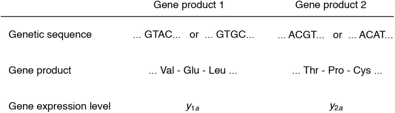