

Abstract
Intracellular processes such as cytoskeletal organization and organelle dynamics exhibit massive subcellular heterogeneity. Although recent advances in fluorescence microscopy allow researchers to acquire an unprecedented amount of live cell image data at high spatiotemporal resolutions, the traditional ensemble-averaging of uncharacterized subcellular heterogeneity could mask important activities. Moreover, the curse of dimensionality of these complex dynamic datasets prevents access to critical mechanistic details of subcellular processes. Here, we establish an unsupervised machine learning framework called DeepHACKS (Deep phenotyping of Heterogeneous Activities in the Coordination of cytosKeleton at the Subcellular level) for “deep phenotyping,” which identifies rare subcellular phenotypes specifically sensitive to molecular perturbations. DeepHACKS dissects the heterogeneity of subcellular time-series datasets by allowing bi-directional LSTM (Long-Short Term Memory) neural networks to extract fine-grained temporal features by integrating autoencoders with conventional machine learning outcomes. We applied DeepHACKS to subcellular protrusion dynamics in pharmacologically perturbed epithelial cells, revealing fine differential responses of leading edge dynamics specific to each perturbation. Particularly, DeepHACKS in conjunction with blebistantin treatment revealed the emergence of rare subcellular and single-cell phenotypes driven by “bursting” protrusion. This suggests that the temporal features directly learned from leading edge dynamics enable fine-grained identification of drug-related phenotypes, which may not be accessible from static cell images. In summary, our study provides an analytical framework for detailed and quantitative understandings of molecular mechanisms hidden in their heterogeneity. DeepHACKS can be potentially applied to analyze various time-series data measured from other subcellular processes.
Introduction
Recent advances in fluorescence microscopy allow researchers to acquire an unprecedented amount of live cell image data at high spatiotemporal resolutions; however, Intracellular dynamics such as cytoskeletal, membrane, and organelle dynamics exhibit massive subcellular heterogeneity, which makes it challenging to fully understand rich microscopy datasets1. Moreover, the traditional ensemble-averaging of uncharacterized subcellular heterogeneity could lead to the loss of critical mechanistic details. For instance, if some cytoskeletal dynamics in only a small subcellular region in a rare cellular subpopulation specifically respond to given perturbations, it will be easily overlooked by the human eye and conventional assays based on ensemble averaging.
In cancer genomics, detecting rare mutations and cell types by deep sequencing has been critical to the understanding of tumor heterogeneity. However, little effort has been made for “deep phenotyping”2,3 in cell biology, which identifies detailed and rare phenotypes of subcellular and cellular processes from microscopy datasets. Particularly, deep phenotyping of subcellular processes can enable us to access critical mechanistic details of molecular processes masked by subcellular dynamic heterogeneity. Over the last decade, image analysis software has facilitated the quantitative measurements of molecular and cellular events from microscopy images at high spatiotemporal resolutions. Still, characterizing phenotypes from their heterogeneity has been mainly focused on static images at a cellular level without capitalizing rich spatiotemporal information.
For effective phenotyping from high dimensional datasets, it is necessary to project raw data onto low-dimensional manifolds to avoid the curse of dimensionality, where statistical analyses cannot reach statistical significance in high dimensions due to the sparsity of data. Therefore, in conventional machine learning settings, the hand-crafted features are extracted for dimensional reduction. Our previous unsupervised ML pipeline4 relied on the hand-crafted time-series feature, ACF (Auto-Correlation Function), to deconvolve the time series heterogeneity from live cell movies 4. Hand-crafted features, however, depend strongly on prior knowledge and are limited in representing large complex datasets comprehensively, preventing the discovery of fine-grained “deep” phenotypes.
Over the last decade, deep learning (DL) had risen to be a mainstream ML method, overcame the performance of traditional ML, and surpassed the human capabilities in many areas 5,6. Unlike conventional ML, DL does not use hand-crafted features, but rather it learns the data representation (features) directly from raw data 7,8. The learned features by DL are better positioned to capture more accurate information from complex datasets, enabling us to unravel the heterogeneity of the data in great detail for deep phenotyping. One drawback of the DL approach, however, is that DL requires large datasets to prevent overfitting, where neural networks fit their training data but are not generalized well. Also, DL is considered to be a black-box approach where the interpretability of learned features is limited. Therefore, the outcomes may not be compatible with human intuition.
To address these challenges, we developed a self-supervised DL framework integrated with conventional unsupervised ML, called DeepHACKS (Deep phenotyping of Heterogeneous Activities in the Coordination of cytosKeleton at the Subcellular level). DeepHACKS allows us to deconvolve the phenotypic heterogeneity of subcellular time-series dataset in a self-supervised manner where DL-based features learning is regularized by traditional ML outcomes. Due to the fine-grained nature of learned temporal features, DeepHACKS allowed deep phenotyping of subcellular dynamics from live cell movies, meaning that we can identify the rare subcellular and single-cell phenotypes, specifically sensitive to molecular perturbations.
We applied DeepHACKS to cell edge dynamics, in which the leading edges of migrating epithelial cells undergo protrusion and retraction cycles under pharmacological perturbation. Growing numbers of studies show the vital roles of cell protrusion, including in tissue regeneration9,10, cancer invasiveness and metastasis11–13, and microenvironmental surveillance of leukocytes14. It has been demonstrated that long-term migratory behaviors of Dictyostelium can be predicted by the short-term morphological changes over the second timescales15. It was shown that the coordination between protrusion and retraction determines metastatic potency16, and influences phenotypic switching of cell migration17. Morphodynamic phenotypic-biomarker can be used for the diagnosis of metastatic potential of breast and prostate cancer 18.
Cell protrusion and retraction involve precise coordination of actin regulators to collectively organize actin cytoskeleton4,19–21. Dissecting such dynamics has been a challenging task due to substantial morphodynamic heterogeneity4,20,21. DeepHACKS quantitatively identified the deep phenotypes of subcellular protrusion from highly heterogeneous and non-stationary-edge dynamics of migrating epithelial cells, revealing fine differential responses of leading-edge dynamics specific to perturbations. Particularly, DeepHACKS revealed the emergence of rare protrusion subcellular and cellular phenotypes upon blebbistatin. Our study suggests that the temporal features directly learned from leading-edge dynamics enable fine-grained identification of drug-related subcellular phenotypes, which can not be accessible from static cell images.
Results
DeepHACKS: deep phenotyping of subcellular protrusion
To deconvolve the heterogeneity of subcellular protrusion activities at the fine spatiotemporal resolution, we developed a computational analysis pipeline, DeepHACKS (Fig. 1), which leverages DL to learn the features in a self-supervised manner using the outcomes from conventional unsupervised learning analysis. Since subcellular protrusion occurs over varying periods of time and creates heterogeneous temporal lengths, we advanced our ML algorithms to include the time series with heterogeneous temporal lengths. DeepHACKS consists of four main components: i) Predefined feature (Autocorrelation Function; ACF)-based clustering, ii) Deep feature learning, iii) Fine-grained subcellular phenotype identification (Deep Phenotyping), iv) Single-cell phenotyping based on subcellular phenotypes. We used the ACF-based clustering to obtain the preliminary cluster labels as the prior information, which is injected into deep feature learning in a self-supervised manner to automatically learn features for deep phenotyping.

(a) Time series data generation and preprocessing. (1-2) Live cell imaging and local sampling. Time-lapse movies of the leading edge of migrating cells treated with/without different drugs were taken at 5 sec per frame, and then probing windows (500 x 500nm) were generated to track the cell edge movement and local velocities were calculated per window. (3-4). Event registration and time series selection. The velocity profile per window was divided into protrusion and retraction events based on protrusion onset. Then all the protrusion intervals with a length longer than 50 sec are selected, and the samples with longer protrusion duration are truncated to 250s for further analysis. (5-6) Random noise padding and velocity transformation. The raw velocity profiles were non-linearly scaled to [-1, 1] for the purpose of convenient training and eliminating the effect of larger values. (b) Pre-phenotyping by conventional ML. ACF-based clustering pipeline was applied to the collected data to identify the protrusion phenotypes. (c) Deep feature Learning. A Guided autoencoder integrates an LSTM-autoencoder and multiple-layer perceptron (MLP) classifier. The optimal weight to balance the contributions of two branches was searched exhaustively and chosen based on drug perturbation analyses. The deep features from the bi-LSTM encoder were extracted for further phenotyping. (d) Phenotyping. Subellular phenotypes were identified by clustering analysis using deep features. Coarse phenotypes can be divided into deep phenotypes for more precise drug characterization. Subcellular phenotypes are used for single-cell phenotyping.
We prepared our sample videos of PtK1 epithelial cells in control and drug-perturbed conditions. Then, we segmented the cell membrane boundary of each frame in each movie and locally divide cell edges into small probing windows with a size 500 by 500nm19,20. Then time series of protrusion velocities were acquired by averaging velocities of pixels in each probing window (Fig. 1a.1-2). After detecting the protrusion onset, the time-series protrusion velocities were aligned as a temporal fiduciary (Fig. 1a.3-4)20. After that, following the same procedure in our previous study4, we denoised the time series velocity profile using Empirical Mode Decomposition (EMD)22 to reduce noise.
Since the temporal lengths of protrusion velocity time series are heterogeneous, calculating the similarity between samples of different temporal lengths is not straightforward. To produce conventional ML-based results (Fig. 1b), we assume that the time series protrusions are dissimilar if the lengths of them are too different. Therefore, instead of calculating the similarity distance among the whole samples, only the distance among samples within similar lengths is calculated. Then, auto-correlation functions (ACFs) as the time series features were used in discovering the novel phenotypes in our previous study (ACF-based clustering, Fig. 1b.8)4. To calculate the ACF-based distance among time series with similar temporal lengths, we padded random noise to the later part of the time series to make the same time length (Fig. 1a.5). We followed the previous ML pipeline, including SAX (Symbolic Aggregate approximation)23 (Fig. 1b.7) and Euclidean-based ACF distance. We pooled all the distance similarity together for partial similarity distance and applied the community detection clustering algorithm24 to determine the distinct clusters of protrusion dynamics (Fig. 1b.9), which serve as the pre-phenotypes for the next step of deep feature learning.
Then, we performed feature learning by leveraging deep learning (Deep Features-based clustering, Fig. 1c). First, we preprocess the time series by rescaling them to the range [-1, 1] to eliminate the effect of large velocity magnitude (Fig. 1a.6). Autoencoder25 has been widely used for feature learning by minimizing the difference between input and output as reconstructed input. One weakness of basic autoencoder, however, is that the features is difficult to interpret since there is no prior information included during the training process. Therefore, many structures26–29 based on autoencoder such as variational autoencoder26 have been proposed. In our feature learning, in order to inject the prior information on the hidden layers, we added another classification branch to make the autoencoder learn features that are consistent with our conventional unsupervised ML analysis. We used bidirectional Long-Short Term Memory (bi-LSTM) structure30,31. Particularly, LSTM specializing in time series data can handle variable-length time series since it does not require a fixed length of time series. By Integrating these concepts, we developed the feature learning framework called Guided Bi-LSTM autoencoder. By optimizing the total loss comprising the loss functions of the autoencoder and the classifier, we trained Guided Bi-LSTM autoencoder using our dataset, including more than 30,000 time-series samples. Then, we applied Principal Compound Analysis (PCA) to reduce the feature dimension and selected the first 15 principal components, which explained more than 95% of the variance.
We used these features to perform clustering analysis to refine the preliminary clustering results with ACF features (Fig. 1d). We generate the different clustering results by varying the balancing weight between the losses of the autoencoder and the classifier and then determine the optimal clustering by evaluating the sensitivity of the clustering results to the reference drug perturbation. Then using the same deep features (features learned from deep learning), we perform sub-clustering analyses for the clusters identified in the previous step. We call these sub-clusters “deep phenotypes” while calling the parent clusters “coarse phenotypes” (Fig. 1d). Then, the deep phenotypes were compared in control and pharmacologically perturbed conditions. Finally, we used the proportions of subcellular protrusion phenotypes as single-cell features to perform clustering analysis to identify single-cell protrusion phenotypes (Fig. 1d).
Pre-identification of subcellular protrusion phenotypes by ACF features
Previously, we used ACF features and density-peak clustering32 to deconvolve the heterogeneity of subcellular protrusion velocity time-series, which led to five distinct clusters 4. Instead, we used the community detection algorithm33 since it can handle the partial similarity distance matrix from unequal temporal lengths. Using Silhouette value34, we evaluated the optimal number of clusters (Fig. 2a). We chose the optimal one as six, which were confirmed visually by the ordered distance maps and the silhouette plots of the clustering results. One difference from our previous results was that we were able to split the previous “fluctuation” cluster into the clusters of “steady” (Cluster I) and “bursting” (Cluster II) protrusions (Fig. 2b). Cluster II showed that edge velocity was changed dramatically within 100 seconds. Therefore, we named it ‘Bursting Protrusion’. Since Cluster III-V exhibited periodic edge velocity, we named them ‘Periodic Protrusion’ and Cluster VI named ‘Acceleration Protrusion’ as we did in our previous work4.

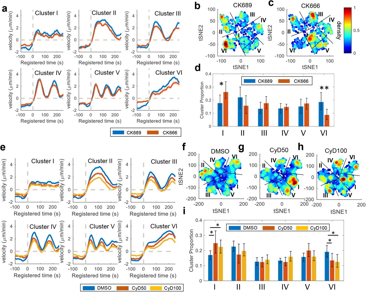
(a) Silhouette plot that determines the optimal number of clusters. The community detection clustering method was applied with varying numbers of nearest neighbors. The maximum silhouette value determined the number of clusters, six. (b) Average temporal patterns of protrusion time series in the clusters whose temporal length is larger than 250s with a 95% confidence interval registered at protrusion onset (t = 0). (c-f) Effects of Arp2/3 inhibitor, CK666 on the subcellular protrusion phenotypes. Averaged protrusion velocity time series in each cluster registered at protrusion onset in CK689 or CK666-treated cells (c). t-SNE plots of autocorrelation functions of protrusion velocity time series overlaid with the density of data in the cells treated with CK689 (d) and CK666 (e). Comparison of the proportion for each cluster per cell between CK689 (50 μM, inactive control compound) and CK666 (50 μM) (f). (g-j) Effects of myosin-II inhibitor, blebbistatin on the subcellular protrusion phenotypes. Averaged protrusion velocity time series in each cluster registered at protrusion onset in DMSO or blebbistatin-treated cells (g). t-SNE plots of autocorrelation functions of protrusion velocity time series overlaid with the density of data in the cells treated with DMSO (h) and blebbistatin (i). Comparison of the proportion for each cluster per cell between DMSO and blebbistatin (20 μM) (j). Solid lines indicate population averages, and shaded error bands indicate 95% confidence intervals of the mean computed by bootstrap sampling. The error bars indicate 95% confidence interval of the mean of the cluster proportions. * p<0.05, and ** p < 0.01 indicate the statistical significance by bootstrap sampling.
Using these updated clustering results, we repeated the analysis of the CK666 (Arp2/3 inhibitor) perturbation to these protrusion phenotypes. Consistently with the previous results, the analysis showed that CK666 significantly reduced the proportion of the accelerating protrusion phenotype (Cluster VI) only in comparison to the inactive control (CK689) (p=0.013 by bootstrap resampling) (Fig. 2c-f and SFig. 1a). Next, we investigate the effects of blebbistatin using the clustering results. First, the velocity profile in Cluster II (Bursting Protrusion) was substantially elevated by blebbistatin treatment (Fig. 2g). Moreover, the quantification of the proportion of the clusters showed that Cluster II was significantly increased by the blebbistatin treatment (p=0.004 by bootstrap resampling) (Fig. 2h-j and SFig. 1b), while CK666 did not show significant effects (Fig. 2f). This suggests that there exist subcellular regions where downregulation of myosin II promotes bursting protrusion.

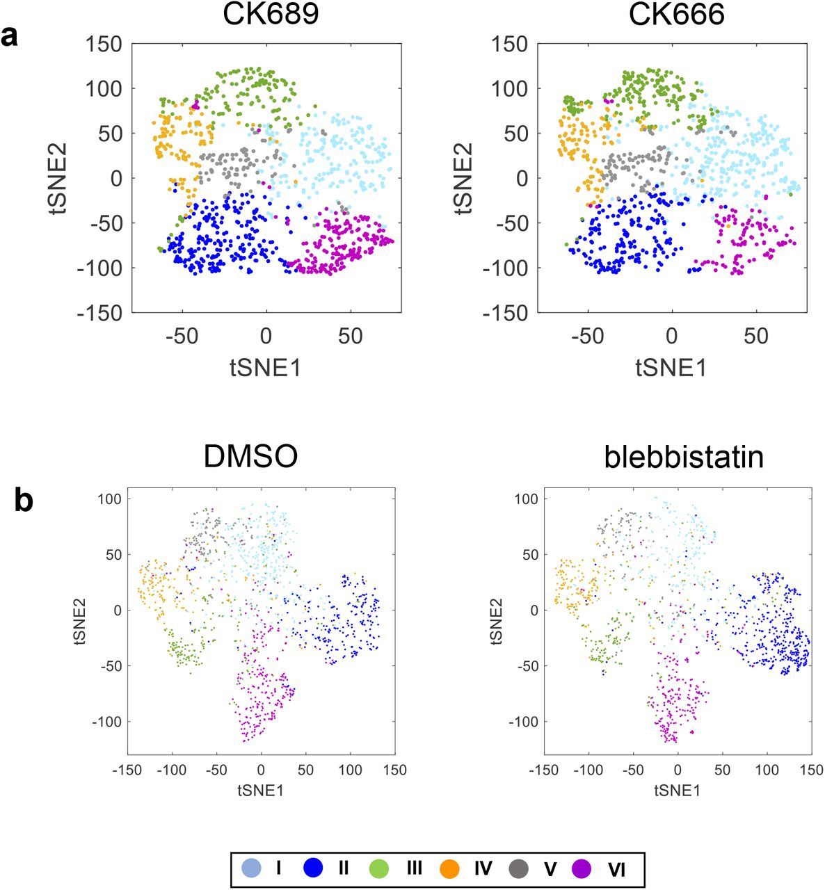
t-SNE plots of ACF features in the conditions of (a) CK689 vs CK888 and (b) DMSO vs blebbistatin
Self-supervised deep feature learning for subcellular protrusion phenotyping
Using the labels from the previous ACF-based clustering results, we trained a Guided Bi-LSTM autoencoder (Fig. 3a). The reconstruction, classification, and total losses decrease as the training epoch increases (Fig. 3b-d). The visual comparison between the input and the output confirmed that the autoencoder training was effective (Fig. 3h-i). After the dimensional reduction of the autoencoder features by PCA (Fig. 3e), we applied community detection to find distinct clusters. We varied the weight parameter balancing the losses of the autoencoder and the classifier and evaluated each clustering results based on the effect sizes of accelerating protrusion (Cluster VI) between CK689 and CK666 (Fig. 3f), and bursting protrusion (Cluster II) between DMSO and blebbistatin (Fig. 3g). The effect sizes of accelerating protrusion (Cluster VI) reached maximum distinctively when the weight parameter is 25, while there is little pattern of the effect size variations of bursting protrusion (Cluster II). This means that finding the optimal weight parameter is critical for the analysis of accelerating protrusion. In contrast, the wide range of the weight parameters is suitable for the analysis of bursting protrusion. Therefore, we chose parameter 25. With the weight parameter, 25, even though the average temporal patterns of protrusion velocities from ACF and Deep feature (DF)-based clustering are identical (Fig. 3j), the tSNE feature visualization revealed their significant differences (Fig. 3k and n). The quality of the clustering from the DF was substantially better than the ACF-based clustering based on the order-distance map and silhouette values (Fig. 3l, m, o, and p). This feature refinement will enable us to perform a more detailed analysis of each protrusion phenotype in the downstream steps.

(a) Deep feature learning of Guided bi-LSTM autoencoder. (b-d) The training performance of feature learning. Total loss (b), auto-encoder loss (c) and classification loss (d). (e) Principal component analysis on the deep features. (f) Effect sizes of the difference between CK689 and CK666 in Cluster VI with varying weight parameters. (g) Effect sizes of the difference between DMSO and blebbistatin in Cluster II with varying weight parameters. (h-i) Visual comparison between the input of scaled velocities (h) and reconstructed output from autoencoder (i). (j-o) Comparison between ACF and DF-based clustering. Average protrusion velocity time series registered at protrusion onset (t=0) (j).). Solid lines indicate population averages, and shaded error bands indicate 95% confidence intervals of the mean computed by bootstrap sampling. t-SNE plot of ACF (k) and DF (n). Ordered distance map from ACF-based clustering (i) and DF-based clustering (o). Silhouette plots from ACF-based clustering (m) and DF-based clustering (p).
Deep Phenotypes of Accelerating Protrusion
In the CK666 perturbation experiments where we optimized the deep feature learning, we were able to identify similar clustering patterns using the deep features (DF) (Fig. 4a) to those from the ACF (Fig. 2c). Also, the drug effects of CK666 on Cluster I and VI (Fig. 4a-d and SFig. 2a) are consistent with the previous ACF-based results (Fig. 2f) (ACF-based clustering, p-value=0.045 for Cluster I and 0.013 for Cluster VI; DF-based clustering, p-value = 0.016 for Cluster I and 0.0069 for Cluster VI by bootstrap resampling). The smaller p-values in DF-based clustering are expected because we selected the weight parameter, which gave the maximal effector size for Cluster VI.

t-SNE plots of DF (Deep Features) in the conditions of (a) CK689 vs CK888, (b) DMSO vs Cytochalasin D, and (c) DMSO vs blebbistatin
(a, e) Average velocity time series registered at protrusion onset (t=0) in each cluster of the cells treated with CK689 or CK666 (a) and DMSO or Cytochalasin D (CyD50: 50 nM, CyD100: 100nM) (e). Solid lines indicate population averages, and shaded error bands indicate 95% confidence intervals of the mean computed by bootstrap sampling. (b-c, f-h) t-SNE plot overlaid with the density of the deep features of the cells treated with CK689 or CK666 (b-c) and DMSO or Cytochalasin D (f-h). (d, i) Comparison of the proportion for each cluster per cell between CK689 (n= 10) and CK666 (n= 10) (d), and DMSO (n= 22) and Cytochalasin D (n=16 for 50 nM, n= 20 for 100 nM) (i). The error bars indicate a 95% confidence interval of the mean of the cluster proportions. *p<0.05, **p<0.01 indicate the statistical significance by bootstrap sampling.
To validate the results, we applied the same deep features to a different drug, Cytochalasin D (CyD), that was shown to affect accelerating protrusion previously4. Cytochalasin D significantly reduced the proportion of Cluster VI (CyD50: p-value = 0.027; CyD100: p-value = 0.013 by bootstrap resampling) (Fig. 4e-i and SFig. 2b). Also, Cytochalasin D significantly increased the proportion of Cluster I (CyD50: p-value = 0.021; CyD100: p-value = 0.023 by bootstrap resampling). Consistently with CK666, we found that the DF-based clustering analysis provided smaller p-values than the previous ACF-based analysis 4, demonstrating that the DF can provide more sensitive and robust statistical analyses.
Next, we performed deep phenotyping of accelerating protrusions (Cluster VI). The previously identified phenotypes are sub-divided to further identify fine-grained phenotypes that are more sensitive to drug perturbation. We isolated the samples from Cluster VI and performing a sub-clustering analysis. The t-SNE suggests that there could exist sub-clusters which could be more sensitive to CK666 (Fig. 5a) and Cytochalasin D (Fig. 5b). The Silhouette value indicated that the optimal number of deep phenotypes of accelerating protrusion was three (SFig. 3a). The deep phenotypes identified in Cluster VI displayed subtle but visually distinct behaviors (Fig. 5c): We identified one weak accelerating cluster (Cluster VI-1) and two strong clusters (Cluster VI-2 and 3). Cluster VI-2 exhibited a brief pause of acceleration before 100s, while Cluster VI-3 had constant acceleration. With this deep phenotyping, Cluster VI-1 was not significantly affected using proportion test by CK666 (p-value: 0.0694, bootstrap resampling) and low doses of CyD (CyD50: p-value = 0.0505; CyD100: p-value = 0.2543, bootstrap resampling). In contrast, the proportions of Cluster VI-2 and 3 were significantly decreased by CK666 (p-value = 0.0049 for VI-2, 0.0012 for VI-3, bootstrap resampling) and CyD (CyD50: p-value = 0.3698 for VI-2, 0.0193 for VI-3; CyD100: p-value = 0.0165 for VI-2, 0.0011 for VI-3, bootstrap resampling). Moreover, the effect of CK666 and CyD on Cluster VI-3 was stronger than Cluster VI-2. For blebbistatin treatment experiment, there was no significant effect on any deep phenotypes of acceleration. These sub-clustering results suggest that DF can be used for deep phenotyping for more accurate drug characterization.

(a) Silhouette plot that determine the optimal number of clusters for deep phenotyping accelerating protrusion. The maximum silhouette value determined the number of cluster, three. (b) Silhouette map of the results of single-cell phenotyping

(a-b) t-SNE plots overlaid with the density of the deep features from accelerating protrusion (Cluster VI) for CK689/CK666-treated (a) or DMSO/Cytochalasin D treated cells. (c-d) Average protrusion velocity time series (c) registered at protrusion onset (t=0) and t-SNE plot for three deep phenotypes of accelerating protrusion. (e, g, i) Average velocity time series registered at protrusion onset (t=0) of the deep phenotypes of accelerating protrusion from the cells treated with CK689/CK666 (e), DMSO/Cytochalasin D (g), and DMSO/blebbistatin (i). Solid lines indicate population averages, and shaded error bands indicate 95% confidence intervals of the mean estimated by bootstrap sampling. (f, h, j) Comparison of the proportion for each deep phenotypes per cell between CK689 and CK666 (f), DMSO and Cytochalasin D (g), DMSO and blebbistatin (j).. The error bars indicate a 95% confidence interval of the mean of the cluster proportions. *p < 0.05, **p<0.01 indicate the statistical significance by bootstrap sampling.
Deep Phenotypes of Bursting Protrusion
We also performed the deep phenotyping to Cluster II (Bursting Protrusion) to uncover more detailed effects of blebbistatin. With the DF, Cluster II was not significantly affected by CK666 (p-value = 0.4577; bootstrap sampling) and CyD (CyD50: p-value = 0.0707, CyD100: p-value = 0.1455; bootstrap sampling). In contrast, blebbistatin significantly increased (p-value = 0.0004; by bootstrap resampling) the proportion of Cluster II, consistent with the previous ACF-based results (Fig. 6a and c). The t-SNE plot of the DF distribution (Fig. 6b and SFig. 2c) displays that blebbistatin did not affect Cluster II uniformly, but rather the subset of Cluster II was highly elevated. Therefore, we performed a sub-clustering analysis of Cluster II. DF-based sub-clustering identified five clusters based on the silhouette values (Fig.6d). These deep phenotypes (Cluster II-1~5) identified in Cluster II were shown displayed distinct behaviors. We found that Cluster II-1 was significantly increased by blebbistatin (p-value < 0.0001, bootstrap sampling) while the other Cluster II-2~5 were not affected (Fig. 6j). This deep phenotyping of Bursting Protrusion isolated Cluster II-1, the only deep phenotypes susceptible to blebbistatin treatment. These results suggest that our deep phenotyping can help to isolate specific phenotypes for better quantitation of drug actions.
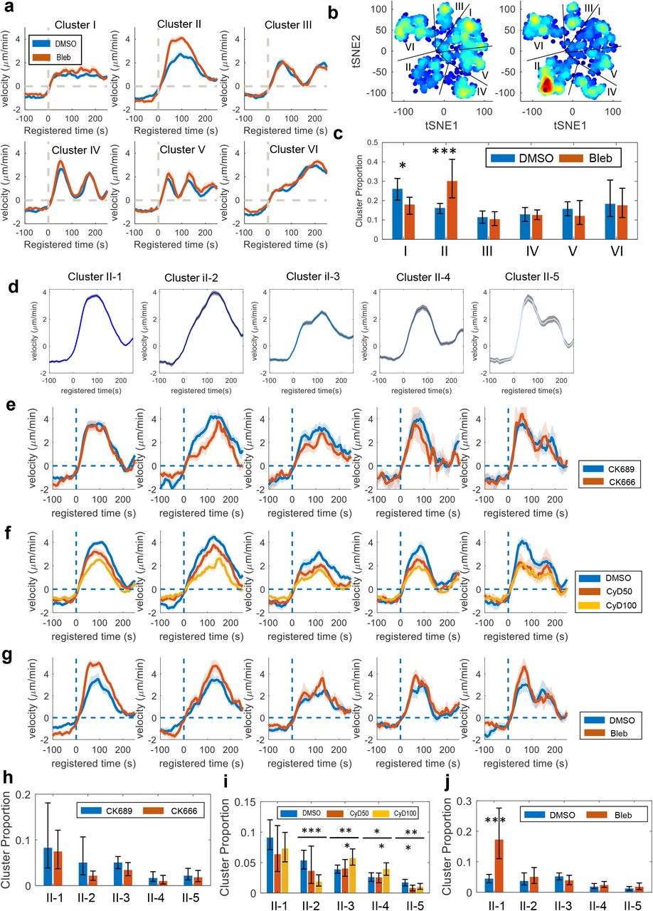
(a) Average velocity time series registered at protrusion onset (t=0) in DF-based clusters of the cells treated with DMSO or blebbistatin. (b) t-SNE plot overlaid with the density of the deep features of the cells treated with DMSO or blebbistatin. (c) Comparison of the proportion for each cluster per cell between DMSO and blebbistatin. (d) Average velocity time series registered at protrusion onset (t=0) of five deep phenotypes of bursting protrusion. (e-g) Average velocity time series registered at protrusion onset (t=0) of the deep phenotypes of bursting protrusion from the cells treated with CK689/CK666 (e), DMSO/Cytochalasin D (f), and DMSO/blebbistatin (g). (f-j) Comparison of the proportion for each deep phenotypes of bursting protrusion per cell between CK689 and CK666 (h), DMSO and Cytochalasin D (i), DMSO and blebbistatin (j). Solid lines indicate population averages, and shaded error bands indicate 95% confidence intervals of the mean computed by bootstrap sampling. The error bars indicate a 95% confidence interval of the mean of the cluster proportions. *p<0.05, **p<0.01, ***p<0.001 indicate the statistical significance by bootstrap sampling.
In contrast to blebbistatin, CK666 treatment did not affect any deep phenotypes of Cluster II significantly. CyD treatment decreased the proportion of Cluster II-2 and 5 significantly (p-value < 0.0001 for II-2 and CyD100, p-value = 0.0059 for II-5 and CyD50) and increased the proportion of Cluster II-3 and 4 significantly (p-value = 0.004 for Cluster II-3 and CyD100, p-value = 0.0149 for Cluster II-4 and CyD100). Due to the opposite effects of CyD on the deep phenotypes of Busting protrusion, the original bursting phenotype (Cluster II) was not shown to be significantly affected by CyD (Fig. 4i). Taken together, we performed deep phenotyping to identify subtle temporal patterns in our protrusion time series dataset and precisely associate them with specific drug perturbations by sensitive statistical analyses.
Single-cell protrusion phenotypes
Based on the subcellular protrusion phenotypes, we characterized single-cell phenotypes. The proportions of subcellular protrusion phenotypes in individual cells were used as cellular features for single-cell protrusion phenotypes. We applied manifold learning, UMAP35, to these single-cell feature distributions and then performed clustering analysis using community detection. The silhouette plots with the varying number of clusters indicated that the optimal number of cell clusters is nine. UMAP 2D visualization (Fig. 7a), the proportion plots of each cluster (Fig. 7b), the ordered-distance plot (Fig. 7d), and silhouette plot (SFig. 3b) demonstrated that the identified cell clusters are highly distinct.

(a-b). UMAP (a) and heatmap (b) of clustered single-cell proportions of subcellular protrusion phenotypes. (c) The ordered distance map of single-cell clustering. (d) Average subcellular protrusion proportions in each cell phenotype. (e) Average proportions of the deep phenotypes of bursting (Cluster II) and accelerating (Cluster VI) protrusions in each cell phenotype. (f-h) Comparison of the proportional differences between Bursting and Steady Cell Groups, and Accelerating and Steady Cell Groups in the conditions of CK689/CK666 (f), DMSO/Cytochalasin D (g), DMSO/blebbistatin (h). *p<0.05, ***p<0.001 indicate the statistical significance by bootstrap sampling.
Each cell cluster was characterized by the mean proportions of subcellular protrusion phenotypes (Fig. 7d). Particularly, Bursting Cells (Cell Cluster 7) and Accelerating Cells (Cell Cluster 9) have high levels of Bursting and Accelerating Protrusion, respectively. Strong-Bursting/Accelerating Cells (Cell Cluster 8) have high levels of both Bursting and Accelerating Protrusion. Mid-Bursting/Accelerating Cells (Cell Cluster 6) have medium levels of them. In Table 1, we summarized the characteristics of these cell clusters and their phenotypic names.
We also quantified the proportions of deep phenotypes sensitive to blebbistatin (Cluster II-1; Bursting-1) and CK666 (Cluster VI-2/3; Accelerating 2/3) in each cell cluster (Fig. 7e). Bursting Cells have high levels of Cluster II-1 (blebbistatin-sensitive) and low levels of Cluster VI-2/3 (CK666/CyD-sensitive). Conversely, Accelerating Cells have a low level of Cluster II-1 and high levels of Cluster VI-2/3. Intriguingly, Strong-Bursting/Accelerating Cells have high levels of both Cluster II-1 and VI-2/3, while they have fewer Cluster VI-1 (CK666/CyD-insensitive) than Accelerating Cells. As summarized in Table 1, as cells have more proportions of bursting or accelerating protrusion, they tend to have more corresponding drug-sensitive deep phenotypes. This suggests that the identified cell phenotypes have differential sensitivities to CK666, CyD, and blebbistatin. To confirm this, we first pooled the cell phenotypes as follows: Cell Cluster #3, 6, 7, and 8 into Bursting Cell Group; Cell Cluster #6, 8, and 9 into Accelerating Cell Group; Cell Cluster #1 and 2 into Steady Cell Group. Since Steady Protrusion was affected by the drugs oppositely to Bursting or Accelerating Protrusion in the previous analysis (Fig. 4d and I, and 6c), we quantified the proportional differences between the cells of Bursting and Steady Cell Groups or Accelerating and Steady Cell Groups. We found that CK666 significantly decreased the proportion of Accelerating Cell Group over Steady Cell Group while it did not significantly change that of Bursting Cell Group over Steady Cell Group (Fig. 7f). Intriguingly, CyD/blebbistatin significantly decreased/increased the proportions of both Bursting and Accelerating Cell Groups over Steady Cell Group (Fig. 7g-h) even though they did not affect Bursting/Accelerating Protrusion in the previous subcellular analysis where every cell phenotype was considered (Fig. 4i and 6c). This demonstrates that both subcellular and cellular phenotyping is necessary to fully understand the heterogeneity of cellular drug responses.
Discussion
We developed a DL-based self-supervised learning framework, DeepHACKS, that can deconvolve the heterogeneity of dynamic phenotypes of cell protrusion, which will enable us to achieve detailed understandings of molecular mechanisms hidden in subcellular and cellular heterogeneity. DeepHACKS takes advantage of deep feature learning to identify rare deep phenotypes susceptible to specific molecular perturbations. The framework can provide a new avenue for better quantifying the effects of drug actions more precisely and comprehensively. Using this method, we refined the drug effects of the previously found ‘acceleration protrusion’. Furthermore, we identified a novel protrusion phenotype called ‘bursting protrusion’, which was specifically enhanced by myosin inhibitor blebbistatin. Myosin can down-regulate leading edge dynamics by assembling large focal adhesion, increasing cortical contractility, and increasing actin retrograde flow, and it has been reported that blebbistatin promotes protrusions in 2D36 and 3D37,38 environments. Our analysis suggests that identifying such specific subcellular phenotypes will enable us to understand the heterogeneity of cell motility and morphodynamics and specifically characterize drug effects at subcellular and cellular levels.
While deep learning achieved many successes in cellular image analyses, its application to cellular dynamics has been limited. Here, we collected more than 30,000 protrusion velocity time series and proposed a Bi-LSTM autoencoder framework to automatically extract temporal features for dynamic phenotyping. Furthermore, we integrated the conventional ML outcomes with a Bi-LSTM autoencoder to learn the features useful for our specific purposes. Integrating prior information with deep learning26–29 is vital for building high-performance machine learning systems. It is particularly crucial for unsupervised learning, where there can be numerous outcomes depending upon selected features. Here, we developed an effective deep learning framework to learn rich features based on prior information. The features learned automatically from our framework enabled deep phenotyping to capture better characteristics of drug effects.
Based on the subcellular phenotypes characterized by DeepHACKS, we were able to identify single-cell dynamic phenotypes. This result revealed previously unknown nine different single-cell phenotypes of protrusion dynamics with differential drug sensitivities. Also, we demonstrated that multi-scale analysis encompassing subcellular to cellular scales would provide us with more complete pictures of the heterogeneity of drug actions. Our study suggests that there can exist a surprising amount of phenotypic heterogeneity in cellular dynamics at subcellular and single-cell levels. Therefore, we expect our deep learning framework, DeepHACKS will unravel such dynamic heterogeneity to identify deep phenotypes and accelerate understanding of the mechanism of heterogeneous cellular or subcellular activities with unprecedented precision.
Methods and Methods
Experimental Description
The cell culture and live cell imaging procedures were followed according to the previous studies (Lee, 2015, Wang, 2018). For the drug treatment experiments, we cultured PtK1 cells on 27mm glass-bottom dishes (Thermo Scientific cat. #150682) for two days and stained them with 55μgml−1 CellMask Deep Red (Invitrogen) following the manufacturer’s protocol. Then we monitored the cell using microscopy. For Arp2/3 inhibition experiments, cells were incubated with 50 μM of CK666 or CK689 (EMD Millipore) for an hour before imaging. For Cytochalasin D experiments, cells were incubated with DMSO or Cytochalasin D (50 or 100 nM) (Sigma) for half an hour before imaging. For myosin inhibition experiments, cells were incubated with 20 μM blebbistatin (EMD millipore, cat. # 023389) for a half-hour before imaging.
Unsupervised Learning Using ACF feature
1. Calculation of partial similarity matrix
After the velocity time series are denoised by Empirical Mode Decomposition (EMD), we pooled the time series whose temporal lengths are similar within the threshold (6 frames; 30 seconds).
We pad random noise to the end of each time series to make the length equal to the longest one. We generate the random noise from the gaussian distribution with the mean estimated by the average value of the last five time points. Then, the missing part will be padded with random noise with the estimated mean and standard deviation.
To reduce the dimensionality of time series, we represented the time series data by Symbolic ApproXimate representation (SAX)39 as described in our previous study4.
We calculate the Euclidean distance based on the autocorrelation coefficient.
Repeat from steps 1) to 4) until all the samples are calculated.
The final distance similarity matrix is the average mean of distance similarity matrix and its transpose to guarantee that the similarity matrix is symmetric.
2. Clustering
We applied community detection method33 to the similarity matrix. First, we made a K-nearest neighbor graph based on similarity distance. Then, we calculated the adjacency matrix and identified the communities using the R package igraph. The number of clusters was estimated based on the silhouette values of clustering results.
Deep Feature Learning by Guided bi-LSTM Autoencoder
1. Velocity time series preprocessing
In this step, we will perform nonlinear scaling of protrusion velocity to reduce the effect of large magnitude of protrusion velocity since the large magnitude may come from less accurate measurement. The majority of velocity magnitude should be less than 10μm/min based on our experience. Therefore, we manually designed a sigmoidal mapping function, 2⁄(1 + e−0.3ν) − 1. After this sigmoidal scaling, the range of the velocity becomes [−1, 1].
2. Model Training
We randomly split the dataset into three parts: training, validation, and test sets with a ratio: 0.49, 0.21, 0.3. The training set was used to fit the parameters of the model, while the validation set was used to select the model with the best fit (the lowest value of the objective function). The details of our proposed guided Bi-LSTM autoencoder were shown in Fig. 2a. Mainly we utilized three layers of bidirectional long short-term memory (bi-LSTM) as an encoder to extract the features and combined another three layers of bi-LSTM as a decoder to reconstruct the input. In order to make the representative features consistent with the clustering results from the ACF-based clustering, we added a multilayer perception (MLP) classifier to guide the training process. The total loss includes two loss functions: reconstruction loss using the mean squared error function from the autoencoder and the classification loss using the multiple-categorical cross-entropy function from the MLP. Furthermore, in order to optimize the balance between cross-entropy from autoencoder and mean squared error from cluster labels, we trained the model with different weights from 1 to 50 and selected the best weight that provides the most discriminative features for CK666 perturbation. We used a training set to fit the parameters with the batch size 128 and 237 epochs. During the training, we monitored the loss in the validation set and use the model parameters for the best performance with the validation set. We used the bi-LSTM encoder to extract the features for the subsequent analysis. TensorFlow was used to implement the guided bi-LSTM autoencoder in Python 3 in Ubuntu 18.04.
Phenotyping Using Deep Features
We extracted the features from the trained bi-LSTM encoder and then applied Principal Component Analysis (PCA) for the dimensional reduction of the learned features. Based on the percentage of the explained variance, the first 15 principal components are used for clustering analysis.
After the feature reduction, the dataset was split into paired experiments: CK689/CK666, DMSO/CyD50/CyD100, DMSO/Bleb. For each paired experiment, we calculated the sample similarity using Euclidean distance and then apply community detection on the selected samples with 51 frames. To evaluate the optimal number of clusters, we applied the external criteria: Davies-Bouldin Index (DBI) and silhouette value to estimate the optimal numbers in each experiment on the pooled control samples. We found that the optimal number of clusters was six.
Deep phenotyping Using Deep Features
After the initial clustering, we further sub-divided the phenotypes of Bursting Protrusion (Cluster II) and Accelerating Protrusion (cluster VI) into deep phenotypes using the deep features. We first pooled all the samples from the target phenotypes from different paired experiments and then applied the community detection to determine the deep phenotypes based on the Euclidean distance. The optimal number of clusters was determined by the maximum silhouette value.
Drug Perturbation Quantification
To evaluate the effect of drug perturbation, we first overlaid the velocity profiles between control and drug-treatment experiment together for each cluster or phenotype and then visually checked the changes of velocity magnitude by drug perturbation. Then, we quantitatively measured the cluster proportion to represent the drug effect. We quantified the proportions of phenotypes in each cell from both conditions. Then the distributions of the proportion were estimated by resampling original cell samples using bootstrp() in Matlab 10000 times. Then, p-values were calculated by estimating the probability that proportion in one condition is greater or less than the other condition. The confidence intervals of each experiment were estimated by Matlab build-in function bootci();
Cluster Visualization
For each paired experiment, we applied t-SNE (t-distribution stochastic neighboring embedding) for visualization with the default parameter (PC number:15, perplexity:30). The sample densities on two-dimensional t-SNE mappings were estimated using the crowdedness of each sample below the radius threshold, which was implemented as scatplot in MATLAB by Alex Sanchez.
Data availability statement
The datasets used in the current study are available from the corresponding author on a reasonable request.
Code availability statement
The datasets used in the current study are available from the corresponding author on a reasonable request.
Author Contributions
C.W. initiated the project, designed the algorithm of deep learning, performed the drug response analysis, and wrote the final version of the manuscript and supplement. H.J.C. designed and performed the live cell imaging experiments, drug perturbation experiments; L. W. performed the clustering analysis of the time series of unequal temporal lengths; K.L. coordinated the study and wrote the final version of the manuscript and supplement. All authors discussed the results of the study
Competing Interests
The authors declare no competing financial or non-financial interests.
Author Information
Correspondence and requests for materials, data, and code should be addressed to K.L. (kwonmoo.lee{at}childrens.harvard.edu).
Acknowledgments
We thank Microsoft for providing us with Azure cloud computing resources (Microsoft Azure Research Award), and Boston Scientific for providing us with the gift for deep learning research. This work was supported by NIH grant GM122012 and GM133725.
References


