

Abstract
Sensory neurons encode information using multiple nonlinear and dynamical transformations. For instance, auditory receptor neurons in Drosophila adapt to the mean and the intensity of the stimulus, change their frequency tuning with sound intensity, and employ a quadratic nonlinearity. While these computations are considered advantageous in isolation, their combination can lead to a highly ambiguous and complex code that is hard to decode. Combining electrophysiological recordings and computational modelling, we investigate how the different computations found in auditory receptor neurons in Drosophila combine to encode behaviorally-relevant acoustic signals like the courtship song.
The computational model consists of a quadratic filter followed by a divisive normalization stage and reproduces population neural responses to artificial and natural sounds. For general classes of sounds, like band-limited noise, the representation resulting from these highly nonlinear computations is highly ambiguous and does not allow for a recovery of information about the frequency content and amplitude pattern. However, for courtship song, the code is simple and efficient: The quadratic filter improves the representation of the song envelope while preserving information about the song’s fine structure across intensities. Divisive normalization renders the presentation of the song envelope robust to the relatively slow fluctuations in intensity that arise during social interactions, while preserving information about the species-specific fast fluctuations of the envelope.
Overall, we demonstrate how a sensory system can benefit from adaptive and nonlinear computations while minimizing concomitant costs arising from ambiguity and complexity of readouts by adapting the code for behaviorally-relevant signals.
Introduction
Sensory receptor neurons transform physical stimuli into neuronal representations. Constraints in neuronal dynamic range and bandwidth result in neural codes that represent some aspects of the stimulus at the cost of others, typically through multiple nonlinear and dynamical computations. For instance, sensory neurons are known to adapt to the statistics of their inputs: Visual systems adapt to the luminance and contrast of a visual scene, and auditory systems to the frequency and intensity statistics of the soundscape (Kastner and Baccus, 2014; Nagel and Doupe, 2006). Adaptation creates energyefficient representations and improves stimulus discrimination (Benda and Hennig, 2008; Fairhall et al., 2001; Finn et al., 2007; Gorur-Shandilya et al., 2017; Laughlin, 1981). Adaptation can act on two properties of the mapping from stimulus to neural response: 1) how inputs are integrated in time and/or space (filtering), and 2) how the integrated input is transformed into spikes (gain) (Atick and Redlich, 1990; Attneave, 1954; Barlow, 1961; Carandini and Heeger, 2012; Laughlin, 1981; Nagel and Wilson, 2011; Zhaoping, 2006). However, while adaptive filtering and gain improve information transmission, they also remove information, for instance about absolute light or sound intensity levels. This introduces ambiguity for neural computations in downstream circuits since the meaning of a spike – the pattern and magnitude of the stimulus it represents – will depend on the stimulus history (Fairhall et al., 2001; Haak and Mesik, 2016; Seriès et al., 2009; Whitmire and Stanley, 2016; Zavitz et al., 2016). This ambiguity is desirable when it introduces invariances to intensity or contrast, but it may distort neural readouts if the adaptation affects behaviorally-relevant stimulus features (Fairhall et al., 2001; Hildebrandt et al., 2015).
Like adaptation, other strongly nonlinear computations are beneficial for making explicit some stimulus features at the cost of distorting others. For instance, the recognition of acoustic signals – such as speech – typically relies on two features of a sound: 1) the carrier, or fast oscillations that define the fine structure of the waveform, and 2) the envelope, relatively slower modulations of the intensity or variance of the carrier. A quadratic output nonlinearity produces responses that depend on the magnitude but not on the sign of an input stimulus. This operation is considered crucial for extracting the envelope but it introduces ambiguity about the structure of the carrier. Importantly, the impact of this ambiguity on decoding depends on the stimulus: For spectrally simple, pure-tone carriers, a quadratic nonlinearity produces frequency doubling responses, from which the stimulus frequency can be easily recovered. However, if the carrier is spectrally complex, the frequency content of the stimulus cannot generally be recovered after a quadratic nonlinearity.
Thus, unbiased measures based on information transmission on generic stimulus ensembles can be insufficient to assess the performance of a neural code because the impact of sensory computations, like adaptation or quadratic nonlinearities, is context-specific. A code’s performance depends on the statistics of the stimuli the system processes, and on the features the system aims to extract from the stimuli to drive behavior (Gomez-Marin and Ghazanfar, 2019).
We address this issue in the auditory receptor neurons of Drosophila melanogaster. Hearing is important for courtship behavior (Coen et al., 2014): Males chase the female and produce a dynamical courtship song by vibrating their wing. The song of Drosophila melanogaster males contains two major modes: The sine song consists of sustained oscillations with a frequency around 150 Hz, and the pulse song consists of regular trains of short pulses that can have two distinct shapes (Arthur et al., 2013; Clemens et al., 2018a). Females — but also nearby males — evaluate both the spectral and the temporal properties of the song to inform social interactions (Deutsch et al., 2019; Li et al., 2018; Versteven et al., 2017). Mechanoreceptor neurons in the fly’s ear (its antenna) must therefore maintain the carrier and the envelope of the song for further processing downstream. In addition to acoustic communication, flies also detect and avoid threats based on sudden increases in the sound envelope (Lehnert et al., 2013).
Flies detect sound using the arista, a feathery extension of the antenna (Fig. 1A). Sound-induced antennal vibrations, but also slow antennal movement induced by wind and gravity, activate a diverse population of stretch-sensitive mechanoreceptors in the antenna’s second segment – the Johnston’s organ neurons (JONs) (Kamikouchi et al., 2009; 2006; Yorozu et al., 2009). While some types of JONs encode slow antennal movement induced by wind- and gravity (JONs C and E) (Yorozu et al., 2009), the JON-A and JON-B subpopulations respond best to fast, sound-induced antennal vibrations in the frequency range of the courtship song (100-400 Hz) and act as the auditory receptor neurons. These auditory JONs perform multiple nonlinear computations that are thought to improve the representation of sounds (Fig. 1B): JONs adapt to the mean and to the variance of receiver movement (Albert et al., 2007; Clemens et al., 2018b; Lehnert et al., 2013). Mean adaptation renders responses robust to slow antennal movement induced by wind and gravity. Variance adaptation corrects for slow intensity fluctuations, which arise during the dynamical social interactions from the strongly directional and distance-dependent sound receiver (Bennet-Clark, 1971; Morley et al., 2012). The extracellularly recorded bulk spiking activity of JONs A and B – the compound action potential (CAP) (Clemens et al., 2018b; Kamikouchi et al., 2009; Lehnert et al., 2013) (Fig. 1A) – exhibits frequency doubling responses for sinusoidals. For instance, a 300 Hz sinusoidal evokes 600 Hz oscillations in the CAP (Eberl et al., 2000; Lehnert et al., 2013; Tootoonian et al., 2012) (Fig. 1B). This frequency doubling can be reproduced mathematically by squaring the sinusoidal, indicating a quadratic transformation for sound across the JON population. Yet another computation performed by JONs is adaptive temporal filtering: the cutoff frequency of the antennal receiver increases with intensity (Nadrowski and Göpfert, 2014) and this effect is linked to the mechanical amplification of low-amplitude sounds in JONs (Albert and Kozlov, 2016; Göpfert et al., 2006; 2005; Göpfert and Robert, 2003).

A Schematic of the early auditory system of Drosophila and recording location. Sound-induced vibrations of the arista induce antennal rotations and activate antennal mechanosensory neurons – the Johnston’s organ neurons (JONs). The compound action potential (CAP) represents the activity of sound-responsive JONs and can be recorded using an electrode inserted into the joint between the 1st and 2nd antennal segment.
B Left: Fast oscillation (carrier, gray line) with a slowly varying baseline (mean, orange line) and slow and fast (gray boxes) fluctuations of the intensity (variance, black line). Right: Schematic illustration of four JON computations evident from the CAP (the response feature that changes in subsequent rows is marked in red).
C Structures of the tested models. The linear-nonlinear (LN, top) model consists of a linear filter followed by a static nonlinearity. The quadratic filter (QF, middle) model consists of a quadratic filter w/o a nonlinearity. The QF-DN (bottom) model is a quadratic filter with a divisive normalization (DN) stage.
D, E, F CAP (black) and model (colored lines) responses of the three different models in C (rows 2-4) for different stimuli (top row). “Noise” (D) corresponds to bandpass filtered white noise with constant intensity. “Step” (E) is noise with step-wise changes in intensity every 100 ms. “Song” (F) corresponds to male courtship song and contains sustained oscillations, called sine song, and trains of transient pulses. Data from one representative fly.
G, H Comparison of the performance (coefficient of determination r2 between the CAP and model response) for the different models and stimuli in C-F (color coded, see legend). Points correspond to recordings from individual flies. The LN model performs poorly for all stimuli. The QF model performs well for stimuli with a constant intensity (noise), but poorly for stimuli with dynamical intensity profiles (step, background, song). The QF-DN model performs well for all stimuli. “Background” is not shown in D-F and is a noise stimulus of mostly constant amplitude with brief changes in intensity (see Fig. S5). Number of flies for noise/step/background/song is 6/5/9/5.
To understand how diverse computations (mean and variance adaptation, frequency doubling, and adaptive temporal filtering) combine in JONs to encode the song’s carrier and envelope, we built a computational model of the JONs based on CAP recordings. We relied on CAP recordings, since they are currently the only readout of JON responses with sufficient resolution and allow all of the above computations to be measured. The model reproduces all major features of the responses for a wide range of stimuli including the courtship song, and shows that different adaptive and nonlinear computations produce an efficient representation of song. That is, a representation that, despite the complexity of the transformation from sound to response in JONs, is easy to read out and allows a reconstruction of the behaviorally relevant features of the song’s carrier and envelope with little ambiguity.
Results
A quadratic filter and a dynamic normalization stage reproduce CAP responses
To fit a model that captures the multiple computations in JONs (Fig. 1B), we recorded CAP (compound action potential, representing the summed activity of many JONs) responses for stimuli with diverse carrier and envelope dynamics (Fig. 1C): Gaussian noise band-pass filtered between 100 and 900 Hz (termed “noise” from here on) with constant intensity (Fig. 1D) or with step-wise modulations in amplitude (Fig. 1E); and the natural courtship song, which exhibits narrow-band carriers and strong amplitude modulations (Fig. 1F).
A common framework for describing the stimulus-response mapping of sensory neurons is the linear-nonlinear (LN) model (Schwartz et al., 2006; Sharpee, 2013) in which the stimulus is 1) linearly filtered to account for temporal integration properties and 2) transformed by a static nonlinearity to account for neuronal threshold or saturation (Fig. 1C, top). However, a LN model fails to reproduce the nonlinear CAP responses (Fig. 1D-F, top, 1G). A quadratic filter (QF, Fig. 1C, middle) reproduces the fine structure of responses to noise stimuli with constant intensity well but fails for stimuli with dynamic switches in intensity (Fig. 1D-G). For instance, the QF output lacks the response transients after intensity steps and the relative intensity invariance of the steady-state responses (Fig. 1E, F). To reproduce this adaptive gain, we added a divisive normalization (DN) stage after the QF (Fig. 1C, bottom). The DN stage was placed at the output of the QF because variance adaptation arises in the JONs after mean adaptation and frequency doubling (Clemens et al., 2018b; Lehnert et al., 2013). The DN stage low-pass filters the rectified QF output to an adaptation signal, which then divides the QF output to normalize the response. Adding the DN stage greatly improved model performance for stimuli with dynamic envelopes, in particular for the courtship song (Fig. 1E, F, H).
We term this two-stage model – consisting of a quadratic filter (QF) followed by a divisive normalization (DN) stage – QF-DN. The model reproduces responses to a wide range of stimuli enabling us to examine how both quadratic filtering and divisive normalization contribute to the representation of song features in JONs. We first focus on the properties of the quadratic filter.
The quadratic filter is a frequency-dependent encoder of sound carrier and envelope
A linear filter corresponds to a set of weights h(τ) for the stimulus s(t-τ) at τ time steps in the past: r(t) = ∑τ h(τ)s(t-τ) (Fig. 1C, top). A quadratic filter also constitutes a set of weights, H(τ1, τ2), but for the product of stimulus values at different delays τ1 and τ2. r(t) = ∑τ1,τ2 H(τ1, τ2) s(t-τ1)s(t-τ2) (Fig. 2A). While a linear filter can be easily interpreted given its set of weights h – for instance, purely positive filters smooth the stimulus while filters with positive and negative lobes are band-pass filters – understanding the stimulus selectivity of a QF directly from its weight matrix H is challenging. We hence approximated the QF in terms of a bank of LN models with quadratic output nonlinearities, obtained through eigenvalue decomposition of H (Fig. 2B, S1) (Berkes and Wiskott, 2007; Lewis et al., 2002). The outputs of all LN models (Fig. 2C, D) in the filter bank are linearly combined to predict the CAP: r(t) = ∑i σi [∑τ s(t-τ)vi(τ)]2. The σi correspond to the eigenvalues of H (Fig. 2E) and provide weights for each LN in the bank, while the filters vi are given by H’s eigenvectors (Fig. 2C). Note that the full model includes additional bias and linear terms but their contribution to model performance is negligible and these terms were therefore omitted in the following analyses (Fig. S1D).

A The quadratic filter (QF) is a matrix H2(τ1, τ2) that contains weights for the product of stimulus values for different τ. τ=0 corresponds to the time of the response and negative values to the time before the response. The filter was fitted to CAP responses to noise presented at 0.5 mm/s. Filter matrix values are color coded (see color bar).
B The QF can be transformed into a bank of LN models with quadratic nonlinearities (pictograms) using eigenvalue decomposition (Fig. S1). Eigenvectors vi correspond to the filters (see C) and the eigenvalues σi correspond to the weight for each eigenvector (see E) in the filter bank. The four eigenvectors with the highest eigenvalues are sufficient to reproduce the performance of the full quadratic filter (Fig. S1D) and form, when combined with the nonlinearity and the eigenvalue, LN1-4.
C Eigenvectors associated with the largest positive (top, v1 and v2, red hues) and negative (bottom, v3 and V4, blue hues) eigenvalues (see E). Each vector was normalized to unit-norm.
D The relationship between the stimulus filtered by the eigenvectors in C and the response is quadratic. v1 and v2 are “excitatory” filter pairs since filter outputs with large magnitude increase the CAP. By contrast, v3 and v4 are “suppressive”. Curves correspond to the average CAP for binned values of the filtered stimulus.
E Sorted eigenvalues of H2. Values for σ1-4 highlighted in color.
F, G Latency of the filters (F) and phase delays between the filters in a pair (G). Dots correspond to individual flies; lines connect data from the same individual. N=6 flies. See also Fig. S2B-D.
H Frequency transfer functions of each filter in C. Each filter pair contains a filter that responds to low frequencies (v1, v4) and a filter that prefers high frequencies (v2, v3).
I, J Frequency tuning of the phase-locked component at twice the stimulus frequency in the model (I) and the CAP (J). Tuning curves were normalized to peak at 1.0.
K, L Responses of the 4 individual LN (2nd row), filter pairs (3rd row), and the full QF (4th row) to 200Hz (K) and 600Hz (L) sinusoidal stimuli (1st row). For low frequencies (K) the four filters combine to produce sustained oscillations at twice the stimulus frequency. For high frequencies (L) the QF phase-locks weakly and responds strongly to the stimulus onset.
All panels except F, G show data from one representative fly. Filter structure is very similar across individuals (see F, G).
Overall, eigenvalue decomposition yields a compact description of the computation implemented in JONs, since four LN models – corresponding to the four highest-magnitude eigenvalues and vectors – are sufficient to reproduce the performance of the QF (Fig. S1B-D).
The four filters in the filter bank representation are well approximated by Gabor wavelets (Fig. S2A-B). The individual Gabor filters have positive and negative lobes and therefore respond only weakly to static stimuli and best to fluctuating inputs (Fig. 2C, S2E). This filter shape accounts for mean adaptation in JONs, which suppresses responses to static deflections of the antenna. Intriguingly, the four LN units in the model form two filter pairs: An “excitatory” filter pair with low latency and a “suppressive” pair with higher latency (Fig. 2C-F). Both filter pairs are similar: The suppressive pair resembles a delayed and sign-inverted version of the excitatory pair (Fig. 2C). Within each pair, the filters are phase-shifted by 90° and form so-called quadrature pair filters (Fig. 2G). This principal filter structure is independent of the stimulus type used for fitting the model (Fig. S3A-D).
Quadrature-pair filters are well known from auditory nerve fibers in vertebrates (Lewis et al., 2002), from complex cells in primary auditory and visual cortex of vertebrates (Rust et al., 2005; Tian et al., 2013) and from motion-sensitive cells in vertebrate visual cortex or in the Drosophila optic lobe (Borst and Helmstaedter, 2015). Canonical quadrature pair filters extract the stimulus envelope, since the responses of each filter in a pair combine to a phase-invariant and smooth output that is proportional to the stimulus energy (Lewis et al., 2002; Rajan et al., 2013). However, the notion of JONs as envelope detectors is at odds with the phase-locking of responses to sound (Fig. 1D-F). This is explained by an asymmetry in the frequency tuning of the filters in each pair (Fig. 2H): Quadrature pair filters only work as envelope detectors for carrier frequencies at which the two filters have similar response magnitude. In JONs, this is the case for frequencies >400 Hz (Fig. 2H, L) and for this high frequency range, each quadrature pair represents the stimulus envelope. Since the inhibitory pair is delayed relative to the excitatory pair (Fig. 2C, F), JONs only respond to transient increases in stimulus energy (Fig. 2L). The filter structure therefore explains aspects of variance adaptation, which induces transient responses, for high frequencies (Clemens et al., 2012; Rajan and Bialek, 2013; Slee et al., 2005). Below 400 Hz however, only one filter per quadrature pair responds strongly (Fig. 2H, K). In this low-frequency range, the QF effectively behaves like two linear filters with a quadratic nonlinearity: It phase-locks at twice the carrier frequency just like the CAP and responds in a sustained manner (Fig. 2I-K). The QF thus reveals two coding regimes present in JONs: for high frequencies (>400 Hz), JONs encode envelope transients, while for low frequencies (<400 Hz), JONs produce phase-locked, more sustained, and frequencydoubling responses (Tootoonian et al., 2012).
Overall, the properties of the quadratic filter contribute to multiple JON computations, including the frequency-doubling, mean adaptation, and variance adaptation at high frequencies. To examine to what extent the nonlinear filter is itself adaptive, we examined how the structure of the quadratic filter changes with intensity.
Adaptive temporal filtering arises from adaptive antennal mechanics
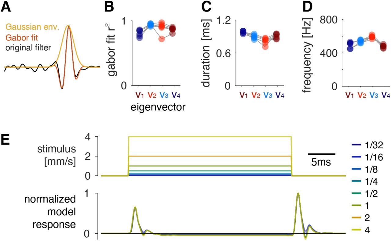
To characterize adaptive processes that shape filter properties, we analyzed QFs fitted to noise stimuli for a range of intensities (1/16 to 4 mm/s, Fig. 3A, B, S4A, B). Eigenvalue decomposition of the different QFs reveals changes in the relative timing and weight (eigenvalues) of the Gabor filters but most of these changes are relatively small (Fig. 3C, S4A). By contrast, a narrowing of the negative lobe of all four Gabor filters leads to an increase in their cutoff frequencies by 200 to 500 Hz over the intensity range tested (Fig. 3D). This increase in the cutoff frequencies with intensity is consistent with predictions from optimal coding theory (Attneave, 1954; Barlow, 1961) and with observations from other systems (Nagel and Doupe, 2006; Zhaoping, 2006).

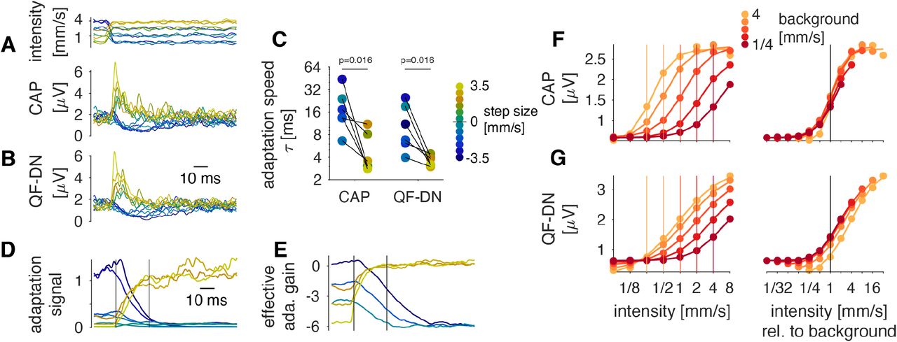
A CAPs (bottom) for a noise patterns (top) of different intensities (color coded, see legend).
B Structure of the quadratic filter (see color bar) at the lowest (left) and the highest (right) intensity tested. The filter structure along the main diagonal narrows with intensity.
C Latencies (top), durations (middle), and phase delays (bottom) of the four leading eigenvectors (filters) v1-4 (color coded as in D) change little with intensity. Lines and error bars represent median±std over 6 flies.
D Shape (top, intensity color-coded, see legend in A) and cutoff frequency (bottom) of the filters v1-4 for different intensities. Filters (top) are from one representative fly. Cutoff frequencies for all filters increase with intensity (r>0.95, p<4×10⁻⁴ for all v).
E Shape (top, example from one fly, intensity color-coded, see legend in A) and cutoff frequency (bottom) for the antennal filter for different intensities. The filter describes the transformation from sound stimulus to antennal movement, and is measured using laser Doppler vibrometry. The cutoff frequency increases with intensity (r=0.97, p=7×10⁻⁵).
F Accounting for antennal mechanics greatly simplifies the filter structure. In the antQF model, the sound was first filtered with the intensity dependent antennal filter (top left) before fitting the QF (top right). The eigenvalue spectrum (bottom) of the resulting quadratic filter reveals that two filters (σ’1 and σ’2) are sufficient to reproduce the structure of the antQF (cf. Fig. 2E).
G Shape (top, example from one fly, intensity color-coded, see legend in A) and cutoff frequency (bottom) for the two dominant eigenvectors of the antQF, v’1 and v’2. The filters are slower and change little with intensity compared to the filters of the original QF (compare D). r=0.18, p=0.7 (left), r=0.81, p=0.016 (right), slope is negligible in both cases (<1.7Hz/intensity doubling). The outliers stem from weak CAP responses to the lowest intensity in one fly (Fig. S4B).
N=6 flies for C-G. P-values from linear fits to the mean across flies.
Thin lines in D, E, G (bottom) correspond to individual flies, the thick line to the median across 6 flies.
Where does this adaptive temporal filtering arise? Previous studies have shown that the frequency tuning of antennal responses to sound is intensity dependent and that this arises from active processes driven by mechanotransducer gating in JONs (Göpfert and Robert, 2003; 2002; Nadrowski and Göpfert, 2014; Riabinina et al., 2011). Measuring antennal movement in response to sound using laser Doppler vibrometry, we confirm that the antenna’s cutoff frequency increases with intensity (Fig. 3E, S4C). To test whether the adaptive antennal tuning fully explains the changes in QF structure, we decomposed the filter into “mechanical” and “neuronal” terms: We first passed the stimulus through the intensitydependent antennal filter obtained through vibrometry (Fig. 3E) – the “mechanical” term – and used this pre-processed stimulus as an input for estimating a new quadratic filter (Fig. 3F), which now captures the remaining “neuronal” processes.
We call this new model “antQF”, short for antennal QF. Accounting for intensity-dependent antennal tuning in the model by prefiltering the stimulus drastically simplifies the structure of the resulting quadratic filter (Fig. 3F): The new quadratic filter only contains slow components associated with the timing of the excitatory and suppressive Gabor filter pairs from the original quadratic filter (Fig. 3B). Eigenvalue decomposition shows that the new quadratic filter is well approximated by only two eigenvectors (instead of four in the original model). The new eigenvectors lack the fast oscillations found in the original filter (Fig. 3G, compare Fig. 3D), demonstrating that these fast oscillations have been captured by the mechanical antennal filters in the antQF. Importantly, the shape and the frequency preference of the two eigenvectors in the antQF are intensity invariant. This demonstrates that adaptive temporal filtering in JONs arises from adaptive antennal mechanics driven by transducer gating, that these antennal mechanics are represented by the Gabor filters in the original QF model, and that the remaining properties of the QF model likely reflect intensity-invariant JON-intrinsic processes. Note that the antQF model is simply a decomposition of the QF model into an intensity-dependent and linear “mechanical” term followed by a quadratic “neuronal” term (Fig. 3F). It is identical to the original QF in terms of the computations it can perform and the outputs it produces.
Divisive normalization reproduces the strength and dynamics of variance adaptation
While the QF explained some aspects of variance adaptation at high frequencies (Fig. 2L), it was not sufficient to reproduce the variance adaptation over the full frequency range (Fig. 2K), for instance for the courtship song (Fig. 1F, H). Our initial model selection (Fig. 1C-H) had revealed that a divisive normalization (DN) stage was required to fully capture the JONs’ adaptive gain (Carandini and Heeger, 2012). In the DN stage (Fig. 4A), the output of the quadratic filter is divided by an adaptation signal – a running estimate of the response gain – obtained by rectification and low-pass filtering the filtered stimulus. Two parameters of the DN stage control adaptation strength σ and adaptation speed τ, and were fitted to the data.

A Internal structure of the divisive normalization stage used to model variance adaptation. The output of the QF is rectified and low-pass filtered to obtain an adaptation signal which divides the output of the QF. τ and σ control adaptation speed and strength, respectively.
B, C Parameters of the model fitted to responses to different stimulus types (“bg” = background stimulus type). Adaptation strength σ (B) changes with the stimulus type but is »1.0 for all stimuli, which indicates near complete adaptation for all types. Adaptation time constants τ (C) do not change with the stimulus type. Dots correspond to individual flies. N=5/9/5 flies for step/background/song. P-values from Tukey-Kramer post-hoc tests after a Kruskal-Wallis test.
D, E, F Stimulus (D), stimulus envelope (E, grey) and adaptation signal from the model (E, black). The adaptation signal lags the changes in stimulus intensity (red arrows). This induces transients in the CAP (F, black) due to over and under compensation of the stimulus intensity (red arrows). Vertical black lines in D-F indicate the switches in intensity. The horizontal red line in F, depicts the CAP’s steady-state response.
G, H, I Same as D-F but for song.
See also Fig. S5.
The adaptation strength σ varies across stimulus types, but all values are »1, consistent with the nearperfect intensity invariance of the CAP amplitude after adaptation (Fig. 4B, S5J-L). The adaptation time constant τ is ~15 ms for all stimulus types (Fig. 4C). The DN stage explains the transient CAP dynamics for stimuli with dynamical envelopes (Fig. 4D-I): After rapid changes in intensity, CAP transients arise because the adaptation signal lags the stimulus intensity through a delay introduced by the low-pass filter in the DN stage (Fig. 4E, H). Through this lagged gain compensation, the adaptation stage briefly overcompensates for fast decreases and briefly undercompensates for fast increases in intensity (Fig. 4F, I). Note, that in the CAP, transients are slower for negative than for positive steps in intensity and our adaptation model shows that these asymmetrical dynamics arises from the multiplicative nature of adaptation with a single time constant parameter (Fig. S5A-E).
Overall, the QF-DN model accounts for the adaptive and nonlinear JON responses using two computations – quadratic filtering and divisive normalization. Each of these computations comes at a cost: The quadratic filter that induces frequency doubling strongly distorts the representation of the stimulus fine structure (carrier); the adaptive filtering could introduce further ambiguity into the code for carrier because the strength with which particular frequencies are transmitted depends on intensity; and adaptation may be too slow or too fast to contribute to an efficient code for transient communication signals like the pulse song. We therefore explored whether and how each of these computations contribute to an efficient representation of communication signals.
The quadratic nonlinearities produce a robust code of the song envelope
We first examined the contribution of the quadratic filter to producing a robust representation of the song’s envelope pattern. Canonical quadratic filters encode the sound envelope (Rajan et al., 2013). However, as shown above, the JON filter does not act as a canonical envelope encoder for the low frequencies typically found in song (Fig. 2H-L). Rather, for the song, the QF acts more like a linear filter with a quadratic nonlinearity and produces frequency doubling responses – each cycle in the song’s carrier induces two cycles in the response (Fig. 1B, 2K). We reasoned that the frequency doubling could improve the representation of the song envelope, since it doubles the temporal resolution of the representation of the envelope and may improve coding of higher envelope frequencies. To test this hypothesis, we set up two simple encoders: one that squares the stimulus just as in JONs and one that simply thresholds the song waveform (Fig. 5A). We then asked how well an optimal linear decoder could reconstruct the song envelope from the responses of these two encoders under varying levels of response noise. To ensure a fair comparison, we normalized responses of the two encoders to have the same average energy before adding noise. Consistent with our intuition, the quadratic encoder transmits more information about the song envelope than the threshold linear encoder (Fig. 5B, C). Thus, the frequency doubling in the CAP improves the representation of the song envelope.
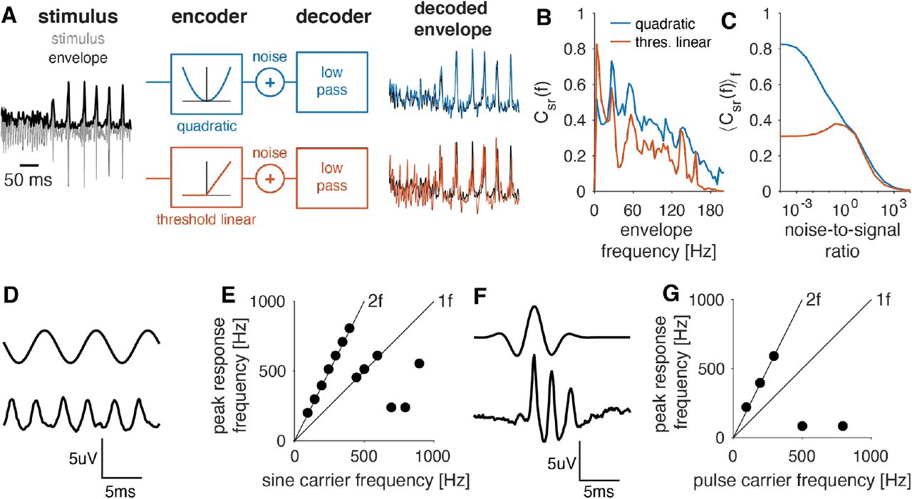
A Encoder-decoder models used to test the role of a quadratic nonlinearity. The song (grey, envelope in black) is passed through a quadratic (blue, top) or a threshold-linear function (red, bottom). Then noise is added, and the response is low-pass filtered to reconstruct the stimulus envelope. Colored lines depict the envelope reconstruction from the quadratic (blue) and the threshold linear (red) encoder, black lines show the envelope of the original stimulus.
B Reconstruction success (coherence Csr(f) between original and reconstructed envelope) for different frequency components of the envelope for quadratic (blue) and threshold linear (red) encoders. The quadratic encoder wins for nearly all frequencies. The noise to signal ratio was 0.25.
C Integral coherence over the range from 1-60 Hz for quadratic (blue) and threshold linear (red) encoders for different noise-to-signal ratios. This frequency range includes the behaviorally relevant interval between song pulses (25-30Hz). The quadratic encoder wins in particular in the low-noise regime. Results are similar when integrating the coherence over the full frequency range.
D 150 Hz sine stimulus (intensity 2 mm/s) (top) and CAP (bottom).
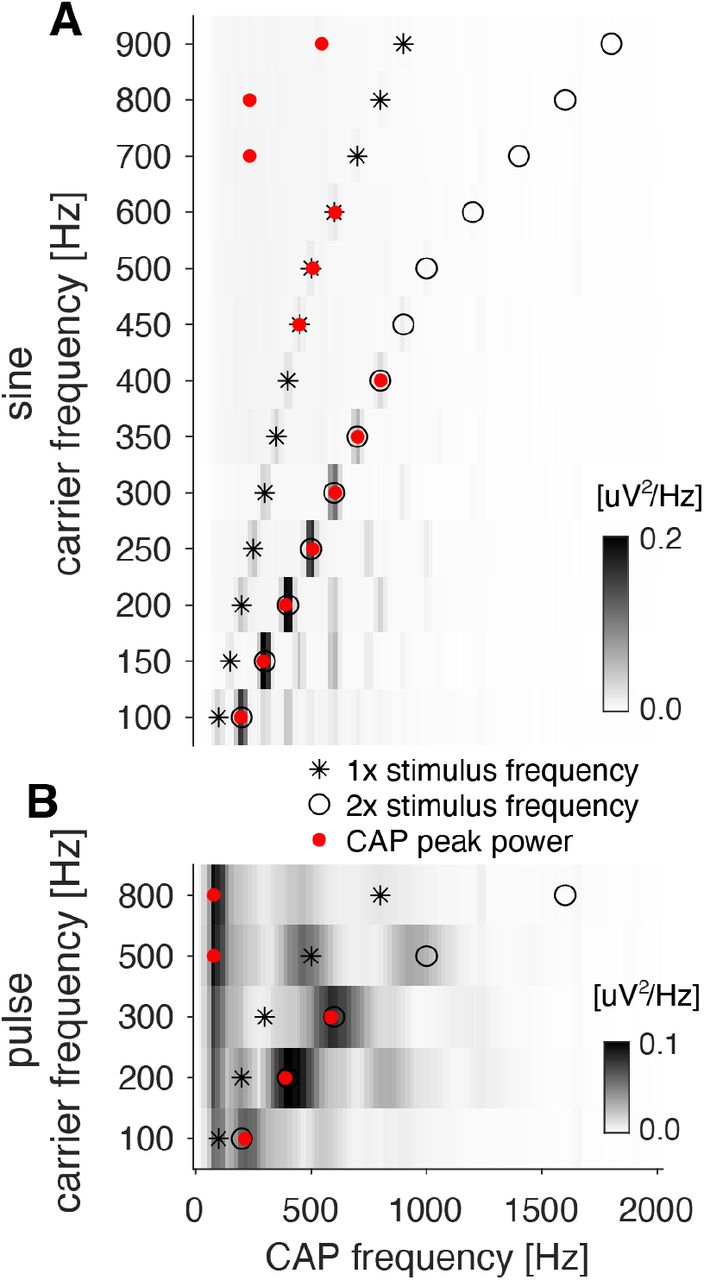
E Dominant frequency of the CAP response for sinusoidals with different frequencies. Lines correspond to peaks at the stimulus frequency (1f) and its double (2f) (see Fig. S6A).
F Pulse with a carrier frequency of 200 Hz (intensity 2 mm/s) (top) and CAP (bottom).
G Same as E but for pulses with different carrier frequencies (see Fig. S6B).
A simple and unambiguous code for communication signals despite an adaptive and quadratic filter
The advantage of a quadratic code for coding the envelope comes at a potential cost when reading out the carrier structure of the stimulus. Generally, a linear system only produces responses with power at frequencies present in the input. For instance, linearly filtering a sinusoid produces another sinusoid of the same frequency with a different gain and phase. This simple mapping is fully reversible even for spectrally complex stimuli. By contrast, a quadratic filter produces power at frequencies that are pairwise combinations of the stimulus frequencies. This includes the frequency doubling seen in the CAP, but also combinations of the different input frequencies. For spectrally complex stimuli, this complicates stimulus reconstruction since it is unclear which response frequencies existed originally in the stimulus and which are the product of the quadratic filter. However, fly communication signals are relatively narrow-band over the duration of the quadratic filter and their dominant frequencies are in the range of phase-locking in JONs (Fig. 5D, F, compare Fig. 2H-K). In this regime, the quadratic filter’s main effect is that of frequency doubling – the dominant frequency in the response is twice of the stimulus carrier frequency. This allows a simple readout of stimulus frequency for the continuous sine song and for the transient pulse song based on half the dominant frequency of the CAP (Tootoonian et al., 2012) (Fig. 5E, G, S6).
Intensity adaptation for song enables robust pattern recognition
Having shown that the nonlinear adaptive code improves envelope coding while still allowing for a relatively simple representation of the sound carrier for the spectrally simple communication signals of Drosophila, we next examined whether the timescale and strength of adaptation are sufficient to enable robust recognition of song pattern across intensities. This is relevant since sound intensity at the female changes drastically during the dynamical courtship because of the angle and distance dependence of the arista (Coen et al., 2016; Morley et al., 2012; 2018). To do this, we employed a classifier which uses the Euclidean distance between responses to classify the identity of short stimulus patterns across intensities (Clemens et al., 2011). We first assessed the ability of the classifier to identify 100 short noise patterns, each presented at 8 different intensities (Fig. 6A). In addition to classifying CAP responses to these stimuli, we also classified model responses, since this allowed us to directly demonstrate the contribution of adaptation by removing the divisive normalization (DN) stage (Fig. 6B, C). Responses of the CAP and the model with DN stage cluster poorly by intensity (Fig. 6D) but very well by pattern identity (Fig. 6E). By contrast, the responses from a model missing the DN stage represent intensity, not pattern identity. Accordingly, the information about stimulus pattern retrieved by the classifier is very high for both the CAP and model with DN stage, reaching ~85% of the maximal information (Fig. 6F). For the model without DN stage, pattern information is strongly reduced. Thus, intensity adaptation enables intensity-invariant classification for noise patterns. However, variance adaptation is incomplete for courtship song (Clemens et al., 2018b), since intensity fluctuations in song can be faster than the adaptation, calling into question whether adaptation can contribute to the coding of song. We therefore also classified stimulus identity for short song patterns of different intensities. We found that the model with DN stage reached near-perfect song pattern identification, while the model without adaptation yielded much lower information values (Fig. 6G). Combined, these results show that adaptation in auditory receptor neurons supports robust, intensity-invariant song-pattern recognition in Drosophila.
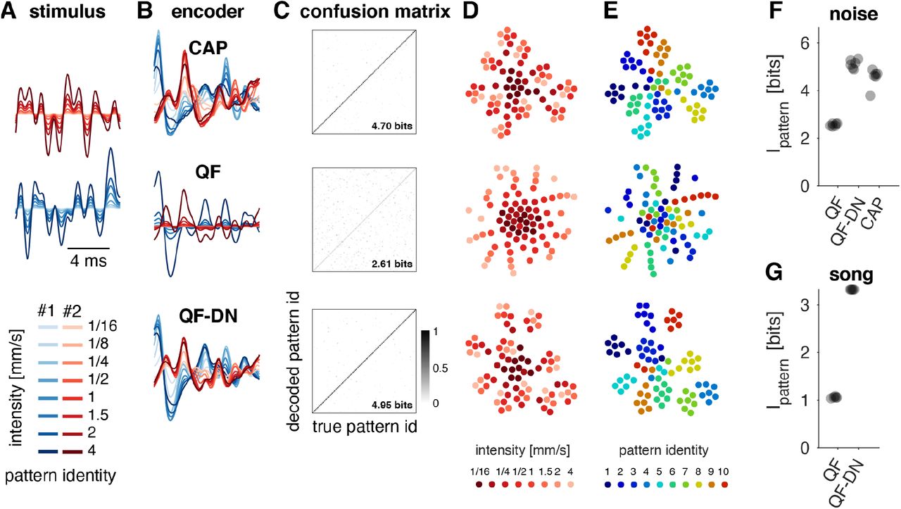
A Two different noise patterns (blue, red) at eight different intensities (color coded, see legend).
B Responses to the noise patterns in A from the CAP (top) and from QF models with (QF-DN, bottom) and without (QF, middle) a divisive normalization stage.
C Confusion matrices (color coded, see color bar) showing the classifier output for 100, 10-ms-long noise patterns presented at 8 different intensities. Diagonal entries correspond to correct classification. Classification performance was quantified using Mutual Information.
D, E tSNE visualization of the CAP, QF, and QF-DN responses for 10 different noise patterns, each presented at 8 different intensities. Responses are color coded by intensity (D) or pattern identity (E) (see legends). In the CAP and in a QF model with divisive normalization, responses cluster by pattern identity (E, top, bottom). In a model without divisive normalization, intensity is encoded by the stimulus magnitude, corresponding to the distance from the center of the point cloud (D, middle).
F, G Pattern information across intensities for noise (F) and song (G) patterns. CAP and QF-DN responses contain more information about pattern across intensities than the QF responses. Dots correspond to individual flies (N=6).
Discussion
Here, we examined how the different computations performed in the JONs affect the representation of song in Drosophila. Based on electrophysiological recordings, we built a computational model that describes the nonlinear and dynamical mapping from sound to the extracellularly recorded population response, the CAP. The model consists of a quadratic filter followed by a divisive normalization stage and fully reproduces CAPs for artificial and natural stimuli (Fig. 1). The quadratic filter acts in a frequency-dependent manner: For high frequencies (>400 Hz), the filter encodes envelope transients, while at the lower frequencies found in the fly’s courtship song, it encodes the envelope but also phase locks to the carrier (Fig. 2). The filter’s preferred frequency increases with intensity and by incorporating direct readouts of antennal movement, we demonstrated that this adaptive frequency filtering arises from antennal mechanics (Fig. 3). Divisive normalization produces the variance (=intensity) adaptation and reveals that response transients after fast changes in sound intensity arise from the adaptation signal lagging behind the stimulus (Fig. 4). Nonlinear and dynamical computations like adaptive temporal filtering and variance adaptation can introduce ambiguities about the carrier and the envelope of sounds, which may reduce coding performance. However, we find that these computations improve the robustness to noise (Fig. 5) and to fluctuations in intensity (Fig. 6) while avoiding strong ambiguities for signals with the statistics of song.
Adaptive and quadratic temporal filtering in JONs
The computation performed by the intensity-dependent quadratic filter at the heart of our JO model can be decomposed into three stages (Fig. 2B, 3F): adaptive temporal filters, quadratic nonlinearities, and combination of excitatory and suppressive quadrature pairs. First, the adaptive Gabor filters determine the intensity-dependent frequency preference of JONs (Fig. 2, 3). By incorporating measures of antennal movement into the model, we demonstrated that the mechanical filtering in the antenna fully explains the adaptive frequency filtering found in the CAP (Göpfert and Robert, 2003; 2002).
Second, a quadratic nonlinearity processes the filtered stimulus and reproduces the frequency doubling responses (Fig. 2K). Since the CAP reflects the bulk spiking activity of all auditory JONs (Clemens et al., 2018b; Lehnert et al., 2013; Łęski et al., 2013), the origin of the frequency doubling and of the quadratic nonlinearity it is still unclear. The frequency doubling could arise in individual JONs that are activated twice during the period of the sound carrier – for instance at negative and positive peaks of a sinusoidal. Alternatively, responses of JONs with different phase preferences could combine in the CAP to produce the frequency doubling (Kamikouchi et al., 2009). Existing anatomical and physiological evidence favors a single-neuron origin of quadratic filtering (Lehnert et al., 2013; Pézier and Blagburn, 2013): Responses from JON subsets from only one side of the JO exhibit frequency doubling (Pézier and Blagburn, 2013), and adaptation to positive steps carries over to reduce responses to negative steps, suggesting that both response components arise in the same neurons (Lehnert et al., 2013). Note that our analyses do not rule out the existence of a subpopulation of JONs that encodes the song’s carrier via linear phaselocking responses. Only comprehensive single-neuron recordings from the population of JONs can resolve this issue.
In the last stage of the QF, the Gabor filters are combined to produce the filter output (Fig. 2C). The Gabor filters form quadrature pairs which are mainly known from higher-order sensory neurons in insects and vertebrates (Borst and Helmstaedter, 2015; Rust et al., 2005; Tian et al., 2013). Interestingly, quadratic filters with the early excitatory and delayed excitatory quadrature pairs found in JONs are also known from the auditory nerve fibers of mammals (Lewis et al., 2002). Typically, quadrature pair filters report stimulus energy at specific frequency bands independent of phase (Rajan et al., 2013). However, to act as an energy detector, the responses of each filter in a quadrature pair must have similar magnitude. In JONs, this is only the case at high frequencies (>400Hz, Fig. 2H, L). For low frequencies, only one of the filters in a pair responds strongly and the quadratic filter produces phase-locked responses (Fig. 2K). The resulting frequency-dependent code preserves information about fine structure for low carrier frequencies through phase locking while maintaining responsiveness to transients in sound energy for high carrier frequencies. Note that this split in coding schemes by frequency could stem from the CAP largely reflecting synchronous activity across the population of JONs (Leski et al. 2013). That is, the lack of a sustained response in the CAP for higher stimulus frequencies may stem from a breakdown of phase-locking, not a reduction in firing rates. However, this is unlikely, since the frequency split is also evident from mechanical responses of the antenna, which are not sensitive to neuronal phase locking but which show strongly reduced sensitivity for frequencies >400 Hz, just like the CAP. The combination of the early excitatory and the delayed suppressive quadrature pair (Fig. 2C-F) produces transient responses for high frequencies in JONs (Fig. 2H-L). In olfactory receptor neurons, a similar delayed-suppressive operation – modeled with a biphasic filter – describes the transformation from transduction current to spiking (Nagel and Wilson, 2011). Whether or not this component of the model maps to the spike generation remains to be tested.
Organization of mean and variance adaptation in JONs
JONs implement two forms of adaptation – to the mean and to the variance of the physical stimulus. Previously, an abstract model backed by experimental data suggested that mean and variance adaptation arise serially in JONs, with mean adaptation occurring before variance adaptation (Clemens et al., 2018b). The more detailed model in the present study confirms this result. Mean adaptation arises in the first stage of the model: The Gabor filters (Fig. 2C) respond only to fluctuating stimuli and do not transmit static or very slow input components corresponding to the stimulus mean (Fig. S2E). The Gabor filters represent active antennal mechanics driven by the gating of mechanotransduction channels (Fig. 3E-G), consistent with previous results that show that mean adaptation is visible at the level of antennal mechanics (Albert et al., 2007). The other form of adaptation found in JONs – to stimulus variance – is produced in two stages in the model: First, the delayed-suppressive operation that combines the two quadrature pairs in the quadratic filter suppresses sustained responses to high frequencies (>400Hz). Second, the divisive normalization in the last stage of the model corrects for sound intensity at low frequencies to produce variance adaptation over the full frequency spectrum (see Fig. 4A, E, H). This is consistent with experimental results that show that variance adaptation arises first in the subthreshold transduction currents (corresponding to the first operation in the quadratic filter) and is completed after spike generation (corresponding to the divisive normalization stage) (Clemens et al., 2018b). The model thus confirms existing experimental and modelling results on the implementation of mean and variance in JONs. In addition, the model constitutes a valuable computational tool for analyzing changes in mean and variance adaptation in genetic mutants to identify the biophysical and anatomical origins of adaptation.
JONs produce an efficient and robust representation of song
Our model demonstrates how different computations – mean adaptation, adaptive temporal filtering, a quadratic nonlinearity, and variance adaptation – contribute to an efficient and robust representation of courtship song features – in particular, the carrier and the envelope (Deutsch et al., 2019) (Fig. 5, 6). First, adaptive temporal filtering (Fig. 3E-H) is consistent with efficient coding principles (Atick, 1992; Attneave, 1954; Barlow, 1961): For weak inputs, the preference for lower frequencies favors integration and sensitivity. For strong inputs, JONs prefer higher frequencies which leads to more differentiation and selectivity. Second, the quadratic nonlinearities produce a representation of the song’s envelope that is robust to noise (Fig. 5A-C), because it pools information from positive and negative stimulus components. Third, mean adaptation (Albert et al., 2007; Lehnert et al., 2013) uncouples the sensitivity of JONs to sound from the baseline position of the antenna (Fig. S2E) – it renders the code for song robust to slow antennal movement from wind or gravity (Clemens et al., 2018b). Finally, variance adaptation produces a representation of the song that is robust to the fluctuations in intensity arising from the dynamical interaction between male and female during courtship (Fig. 6). Adaptation acts as a high-pass filter whose cutoff frequency is set by the adaptation time constant (Benda and Herz, 2003). In JONs, adaptation is fast (Fig. 4), but not too fast – it is sufficiently fast to compensate for the slower (<20Hz) intensity fluctuations that arise from the constant changes in position of the singing male relative to the female during courtship (Coen et al., 2014). But it preserves the behaviorally relevant intensity fluctuations associated with the periodical envelope of the fly pulse song (>20Hz, (Deutsch et al., 2019)).
The code for behaviorally relevant classes of sounds is simple despite a complex encoding scheme
The sequence of highly nonlinear and dynamical computations in JONs results in a complex mapping from sound to JON response. A faithful reconstruction of carrier and envelope from this representation is impossible for arbitrary sounds, because quadratic coding and adaptation combine to produce an ambiguous and stimulus-dependent code. However, sensory neurons like JONs do not serve as general and faithful encoders of stimuli but to extract specific features from behaviorally relevant classes of sensory signals. Hearing in flies is known to be used for acoustic threat detection and for acoustic communication (Kamikouchi et al., 2009; Lehnert et al., 2013). We find that for these signal classes, the relevant stimulus features can be extracted from JONs using relatively simple computations despite a complex encoding scheme.
In the context of acoustic threat detection, sudden increases in sound energy trigger startle responses (Lehnert et al., 2013). JONs accentuate increases in sound energy at frequencies >400 Hz through the quadratic filter (Fig. 2L) and at lower frequencies through variance adaptation (Fig. 4). Information relevant for acoustic threat direction can therefore be read out directly from the amplitude of JON responses by postsynaptic neurons like the giant fiber neuron to trigger startle responses (Pézier and Blagburn, 2013). When evaluating the courtship song, flies are sensitive to a wide range of features of the envelope and the carrier (Batchelor and Wilson, 2019; Deutsch et al., 2019). The envelope pattern can be obtained by low-pass filtering the JON responses (Fig. 5A-C) and this operation is likely performed in neurons directly postsynaptic to the JONs (Clemens et al., 2015; Yamada et al., 2018). For instance, synaptic currents from JON into AMMC-A2 in the fly brain are low-pass filtered by the synapse and the postsynaptic membrane to explicitly encode the envelope (Azevedo and Wilson, 2017). This sequence of transformations resembles the root mean square algorithm in which a signal is first squared and then low-pass filtered to extract the envelope. The code for carrier is highly ambiguous for arbitrary sounds due to the adaptive temporal filtering and the quadratic nonlinearities (Fig. 2, 3). However, for the narrow-band and low frequency (100-400Hz) courtship song, the code for carrier reduces to amplitude scaling from adaptive filtering (Fig. 2H, 3D) followed by frequency doubling from the quadratic nonlinearity (Fig. 2K). From this relatively simple temporal code, the carrier frequency of courtship song can be decoded as half of the dominant frequency in the JON response (Fig. 5D-G, (Tootoonian et al., 2012)).
Conclusion
Overall, our study highlights the importance of examining sensory systems in the context of behaviorally relevant signals. JONs produce a highly dynamical and nonlinear code for sound. This code prevents a faithful reconstruction of general classes of sounds in the fly brain. However, JONs function to represent specific features from particular classes of sounds. For these behaviorally relevant sounds, the relevant features are simple to decode. This match between the behaviorally-relevant signals and the neural code is assumed to be a general feature of neural codes (Ryan and Cummings, 2013; Wehner, 1987). We here show that shaping a code towards the relevant signals, allows animals to avoid the costs of strong nonlinearities in the form of ambiguity and complex decoding while benefitting from improved noise robustness and intensity invariance.
Methods
Flies
Virgin females of the Drosophila melanogaster wildtype strain CantonS Tully were used for all recordings. Flies were sexed and housed in groups of ~10 at 25°C and a 12:12 dark-light cycle. All experiments were performed 2-5 days post eclosion.
Stimulus design and presentation
Stimuli were generated at a sampling frequency of 10 kHz. Band-limited Gaussian noise (from now on termed “noise”) was produced from a sequence of normally distributed random values by band-pass filtering using a linear-phase, finite impulse response filter with a pass band between 80 Hz and 1000Hz. The effect of intensity on JON responses was estimated using 5 independent noise patterns that lasted 5 seconds and were presented at intensities of 1/16, 1/8, ¼, ½, 1, 1.5, 2, and 4 mm/s (“noise” stimuli in Fig. 1). For probing adaptation, we switched the intensity of the noise every 100ms in a sequence that contained all transitions between ¼, ½, 1 and 2 mm/s (“step” stimuli in Fig. 1). The effect of adaptation on intensity tuning was assessed using a noise stimulus at intensities ¼, ½, 1, 2, 4 mm/s (adaptation background) whose intensity was switched every 120 ms for 20 ms to a probe intensity of 1/16, 1/8, ¼, ½, 1,2, 4, and 8 mm/s (“background” stimuli in Figs. 1G, H). To minimize artifacts from abrupt changes in sound intensity, each intensity switch in the step and background stimuli had a duration of 1 ms during which the intensity was linearly interpolated to the new value. We also assessed responses to natural courtship, recorded from a Drosophila melanogaster male courting a virgin female (Arthur et al., 2013; Coen et al., 2014) (“song” stimuli).
Sound
The sound delivery system consisted of i) the analog output of a DAQ card (PCI-5251, National Instruments), ii) a 2-channel amplifier (Crown D-75A), iii) a headphone speaker (KOSS, 16 Ohm impedance; sensitivity, 112 dB SPL/1 mW), and iv) a coupling tube (12 cm, diameter: 1 mm).
The stimulus presentation setup was calibrated as in Clemens et al. (2015). Briefly, the amplitude of pure tones of all frequencies used (100-1000Hz) was calibrated using a frequency-specific attenuation value measured using a calibrated pressure gradient microphone (NR23159, Knowles Electronics Inc., Itasca, IL, USA). To ensure that the temporal pattern of the noise stimuli was reproduced faithfully, we corrected the presented noise patterns by the inverse of the system’s transfer function, measured using a pressure microphone (4190-L-001, Brüel & Kjaer) that was placed at the position of the fly head during recordings.
Electrophysiology
Extracellular recordings were performed using glass electrodes (1.5ID/2.12OD, WPI) pulled with a micropipette puller (Model P-1000, Sutter Instruments). The fly’s wings and legs were removed under cold anesthesia and the abdomen was subsequently fixed using low-temperature melting wax. The head was fixed by extending and waxing the proboscis’ tip. The preparation was further stabilized by applying wax or small drops of UV-curable glue to the neck and the proboscis. The recording electrode was placed in the joint between the second and third antennal segment and the reference electrode was placed in the eye. Both electrodes were filled with external saline (Murthy and Turner, 2013). The sound delivery tube was placed orthogonal to the arista on the side we recorded JON activity form, at a distance of 2 mm. The recorded signal was amplified and band-pass filtered between 5 and 5000 Hz to reduce high frequency noise and slow baseline fluctuations induced by spontaneous movement of the antenna (Model 440 Instrumentation Amplifier, Brownlee Precision). We ensured that the band-pass filter did not distort the recorded signal, e.g. it did not introduce artefactual response transients. We subsequently digitized the recorded signal at 10 kHz with the same DAQ card used for stimulus presentation (PCI-5251, National Instruments).
Laser-Doppler vibrometry
Arista movement was measured using laser-doppler vibrometry (Polytec OFV534 laser unit, OFV-5000 vibrometer controller, Physik Instrumente, low-pass 5 kHz).
Data analysis
Pre-processing
The instantaneous amplitude of the CAP was estimated from the envelope of the recorded signal as the magnitude of the Hilbert transform (Fig. S5A). Tuning curves from the “background” stimui were obtained by averaging the CAP amplitude over the first 8 ms of the probe intensities (see stimulus description above).
Adaptation time scale and strength
The adaptation time scale was estimated from the CAP amplitude traces by fitting an exponential function r(t)=r0 + rmax exp(-t/τ) to the falling/rising phases of positive/negative transients after a change in intensity from the “step” stimuli (Fig. S5C).
Modelling
Model Structure
To reproduce the transfer function from stimulus waveform to CAP waveform, we use the discretized Volterra series, which decomposes the transfer function into a constant term ho, a linear term h1, a quadratic term H2, and higher-order terms ε which we do not consider here:
 s(t) and y(t) are the stimulus and the CAP response, respectively. ho describes a constant offset or bias. h1 is a linear filter and describes how stimulus values τ time steps into the past are weighted in the response. H2 is a quadratic filter and describes how the product of stimulus values at two different time steps in the past, τ1 and τ2, are weighted in the response. The linear models in this paper only include the ho and the h1 term. The quadratic filter model (QF) consists of all terms up to and including H2. The temporal support of the filters h1 and H2, τmax, describes the memory of the system and was set to 10 ms. This duration saturates performance – in initial tests, longer τmax did not improve model performance. This is confirmed by the lack of filter structure in h1 and H2 for τ>8 ms (Fig. 2A).
Model fitting
The individual terms of the model – ho, h1 and H2– were estimated using linear regression: y’(t) = σ(t)w, where y’is the predicted response and w is a concatenation of the model coefficients; [h2, h1, h2]. Exploiting the symmetry of the quadratic filter, H2(τ1, τ2) = H2(τ2, τ1), h2 is a vector containing all upper triangular values including the diagonal of H2 (τ1≥τ2). Equivalently, σ(t) is a concatenation of the inputs for each of the model terms: [s0, s1, s2]. For the bias ho, the input s0=1. For the linear filter h1, the input s1(τ) corresponds to the stimulus in the 10 ms preceding the response time t: s1(τ)=s(t-τ) for all τmax≥τ≥0. To reduce the number of filter coefficients to be estimated, we projected s1 onto a basis composed of 50 Gaussian bumps with a standard deviation of 0.2 ms (2 samples) and a spacing of 0.2 ms (2 samples), with the first bump at 0 ms and the last bump at 10 ms. For the input values to H2, we take the outer product of the stimulus values in the 10 ms (100 samples) preceding the stimulus to be predicted: S2(τ1, τ2) = s(t-τ1)s(t-τ2). To reduce the number of filter coefficients, we projected each matrix onto a basis composed of two-dimensional Gaussian bumps, each bump with a standard deviation of 0.3 ms (3 samples) and a spacing of 0.2 ms (2 samples) (cf. Rajan et al. (2013)). We exploit the symmetry of S2 and keep only the unique values of S2 for which τ1≥τ2, flattened into a vector s2. The projection onto Gaussian bump bases and the exploitation of symmetry reduces the number of free parameters from 1+100+100*100=10101 to 1+50+(502+50)/2=1275.
All filter coefficients were then fitted using ridge regression. Ridge regression minimizes the mean-squared error between the data and the predicted responses and the norm of the filter coefficients: ∑t (y-y’)2+ α∑i wi2 (Tikhonov and Arsenin, 1977). The first term increases the match between the data and the model, the second term penalizes filter weights that do not contribute to improving this match. α controls the influence of the penalty term and was chosen using methods and code from (Park and Pillow, 2011). Since song is relatively sparse, we only used samples that were within ±100 ms of song for model fitting and evaluation. For visualization and analysis of the filters, h1 and H2 were projected from the basis of Gaussian bumps back into the temporal domain.
For models that only contain the first two terms (ho, h1), so-called linear-nonlinear models, we estimate an output nonlinearity based on methods described in (Schwartz et al., 2006). For the quadratic models, the nonlinearity was approximately linear and did not improve performance. We therefore omitted that step to simplify model interpretation.
Fitting the antennal filters and the antQF model
The transfer function from stimulus to antennal movement for each intensity was fitted as a discretized Volterra series with terms ho, h1. This model typically explained more than 90% of the variance in antennal responses to noise (Fig. S4C). To account for intensity-dependent antennal filters in the quadratic model, the intensity-specific antennal filters obtained from one animal were used to pre-filter the stimulus before fitting the quadratic model. This was necessary, because simultaneous measurement of antennal movement and CAP responses was not possible in our rig. However, antennal filters are virtually identical across animals (pairwise Pearson correlation of the filters r=0.97±0.03 across N=5 flies; filters from different intensities were concatenated before calculating the correlations).
Fitting QF-DN
The divisive normalization (DN) stage has the form: x’ = x/(σ + y) where γ is the gain control signal that divides the input x and is given by: γ(t) = ∫ dv || x(t – v) || e−t/τ. τ is the adaptation time constant. The input to the DN stage, x, is the output of the quadratic filter. The QF-DN model was fitted using an iterative procedure: We initialized the filter by fitting a QF model without the DN stage to the data using ridge regression. Then, we optimized the parameters of the DN stage, σ and γ, by minimizing the mean squared error between the CAP and the model prediction using the matlab function “fmincon”, holding the filter coefficients constant. Lastly, we optimized the filter coefficients, holding the DN parameters constant. The model parameters typically converged after 1-2 cycles of fitting the parameters of the DN stage and the filter. During the fitting, only the magnitude, but not the structure of the filter changed from its initialization.
Model evaluation
Model performance was quantified using the squared Pearson’s correlation coefficient between the CAP and the model predictions. Initial experiments with cross-validation show that train and test performance are within ±1% of each other.
QN representations
To gain insight into the computational structure of the quadratic filter, we presented H2 by its eigenvalue decomposition: H2 = ∑i σi vi, viT, where the vi, and σi are the eigenvectors and their associated eigenvalues (Berkes and Wiskott, 2007; Lewis et al., 2002). This representation is useful, since H2 is typically of low-rank, that is few eigenvector-eigenvalue pairs are sufficient to reconstruct H2 with sufficient fidelity (Fig. S1). This representation is equivalent to a bank of linear-nonlinear models with filters vi and quadratic nonlinearities y’ = ∑i σi (∑τ vi(τ)s(t-τ))2.
Subspace overlap
To compare quadratic filters fitted to different stimuli in a manner that is robust to noise, we computed the overlap between the subspaces spanned by the four leading eigenvectors. Specifically, given two quadratic filters A and B, with eigenvectors  and
and  , the cumulative overlap between the pairs of the K largest eigenvectors is given by
  (Fig. S3D) (Romo and Grossfield, 2011).
Envelope reconstruction
To assess the contribution of the quadratic filter to encoding the envelope, we compared the performance of two simple encoders: A rectified linear one, which thresholds the stimulus at 0, and a quadratic one, which squares the stimulus. For a stimulus that is symmetrical around 0, the quadratic encoder will produce more response energy, since the rectified linear one cuts off all negative stimulus components. We therefore normalized the output of each of the encoders to unit norm. Gaussian noise with standard deviation σ was then added to the normalized outputs and the coherence between the model output, r, and the original envelope, e, was estimated from the stimulus: Cer(f) = PerPre/(PeePrr) for different noise-to-signal ratios as a measure of decoding accuracy.
Pattern classification
For pattern classification, we used leave-one-out nearest-neighbor classifier. Each of 100, 10-ms-long response patterns was selected as a template and assigned to the class of its nearest neighbor, based on the Euclidean distance to the 99 non-template patterns (Machens et al., 2003). This resulted in a confusion matrix p(s, s’), which tabulates the joint probability with which a response that was elicited by stimulus s was classified as being elicited by any of the stimuli s’. The mutual information of p serves as a lower bound on the mutual information between stimulus and response: I(s, r)≤I(s, s’)=∑p(s, s’) log2 p(s, s’)/(p(s)p(s’)). I(s, s’)=0 if p(s, s’) is uniform, that is if there is no correspondence between the actual and the classified stimulus. The maximal value of I(s, s’) is given by the log2 of the number of stimulus classes (log2(100)=6.64 for pattern, log2(8)=3 for intensity) for a perfect, one-to-one mapping between stimulus and response. We visualized the similarity structure of the representations using tSNE of a random subset of 10 patterns (Maaten and Hinton, 2008).
Supplemental Figures

A Quadratic filter fitted to a noise stimulus (intensity 0.5 mm/s).
B, C Eigenvalue spectrum of H (B) and cumulative sum of squared eigenvalues (C). The latter corresponds to the fraction of variance in H explained. The four eigenvalues with the largest absolute values are marked in color.
D Performance of QF models using different low-rank approximations of H. The rank corresponds to the number of eigenvalues used for representing the quadratic filter, equivalent to the number of LN models in the filter bank. The left-most bar (pink) corresponds to a rank-0 model, that only contains a bias and linear term, but no quadratic terms. A rank-4 model (with 4 LN models, black outline) is the simplest model with performance close to that of the original full-rank model. Bars show mean over flies and dots show values for individual flies connected by lines (N=6 flies).
E-H Outer product matrix, Vi = viviT, of each of the four leading eigenvectors. The waveforms aligned with the x and y axes show the eigenvectors Vi (right).
I-J Sum of the outer-product matrices (weighted by the eigenvalues) for the pairs of excitatory (I, σ1V1+σ2V2) and suppressive (J, σ3V3+σ4V4) eigenvectors. The matrix in J is sign-inverted, since σ3 and σ4 are negative (See B).
K A rank-4 approximation, given by the sum of all 4 outer products  , yields a good reconstruction of H (compare A, D).
A The waveforms show an example fit (red) to one of the filters (black). The orange trace shows the Gaussian envelope of the filter.
B The performance r2 for the fits of the Gabor filters to the eigenvectors v1-v4 of H.
C, D Duration (C) and carrier frequency (D) of the Gabor filters fitted to v1-v4. Dots show and lines connect recordings of individual flies (N=6 flies) in B-D.
E QF output (top, normalized to peak at 1.0) for the static step stimuli with different intensities (top, intensity is color coded, see legend). The QF responds to the onsets and offset of the step stimuli. This lack of responses to static stimuli is a correlate of mean adaptation.
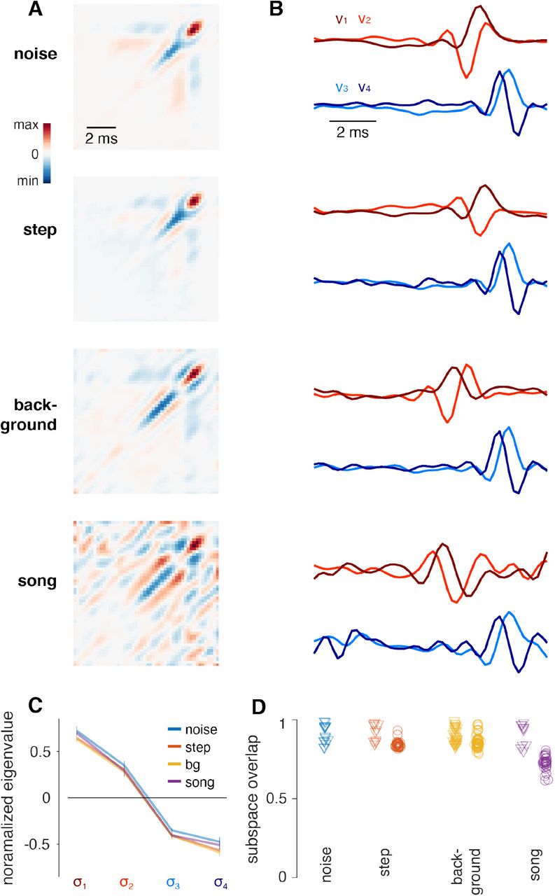
A, B Quadratic filter (A) and four leading eigenvectors v1-v4 (B) for the four stimulus types used in this study.
C Normalized eigenvalues of the QFs in A for the four stimulus types (“bg” = “background” stimulus). The four eigenvalues for each stimulus type were normalized to unit norm to account for differences in filter magnitude. Lines and error bars indicate mean ± std over flies. The relative amplitude of the eigenvalues is independent of stimulus type.
D The subspace overlap measures the match of the hyperplane spanned by the four filters of models fitted to different stimuli (B). We take the filters fitted to noise as the reference. Triangles correspond to the subspace overlap for filters estimated for the same stimuli in different flies and reflect inter-individual variability. Circles indicate the overlap of filters estimated for different stimuli with those estimated for noise. N=6/5/9/5 flies for noise/step/background/song. The filter structure is robust to the stimulus type, indicated by the strong overlap between the subspaces spanned by filters fitted to different stimuli.

A Eigenvalues of the QF, σ1-σ4, fitted to noise stimuli of different intensities.
B Performance (r2) of the QF (black) and the antQF (blue) for different intensities. Each line marks the performance for a given fly. Except for one outlier recording both models perform identically, highlighting the computational equivalence of the QF and the antQF models.
C Performance of the linear filter model that describes the transformation from sound stimulus to antennal position for each intensity. Each line marks the model performance for a given fly across intensities.
D Eigenvalues of σ’1 (brown) and σ’2 (green) of the antQF model for different intensities.
Lines and error bars in A and D indicate mean± std over 6 flies.

A-B Response magnitudes (CAP envelopes) for white noise with intensity steps (top) in the CAP (A) and the QF-DN model (B). Both the CAP and the model exhibit asymmetrical adaptation dynamics: Relaxation to steady state is fast for positive steps (yellow hues) and slower for negative steps (blue hues). See legend in C for color code.
C The effective adaptation time constant in CAP and model response are larger – adaptation is slower – for negative steps than for positive steps (blue and yellow points, respectively, see legend). Note that this is despite the model having a single, fixed parameter for adaptation speed (B). P-values from one-sided sign test (matched pairs are stimuli with same step size with diff sign, black lines) for model and data.
D, E Linear adaptation signal (D) and the effective adaptation gain (E), given by the log of the adaptation signal for the model responses in B. Vertical lines in D mark the beginning and end of the adaptation transients of the adaptation signal from D the model. While the adaptation signal itself is relatively symmetrical for increases and decreases in intensity (D), the effective adaptation gain – proportional to the logarithm of the adaptation signal – exhibits the asymmetrical dynamics of the CAP (E).
F, G Intensity tuning curves of the CAP (F) and the QF-DN model (G), adapted to different background intensities (color code, see legend). Tuning curves are plotted on an absolute intensity scale (left, vertical colored lines indicate background intensities) and with intensity given relative to the background (vertical black line at 1.0 depicts the background). In both the model and the data, tuning curves shift with the adaptation proportional to the background intensity.
A, B CAP power spectra for sine tones (A) and pulses (B) with different carrier frequencies (y-axis) (spectral power of the CAP is color coded, see color bars). The carrier frequency and its double are marked as stars and open circles, respectively. The frequency of maximum CAP power is marked with a red dot. See Figs. 5D-G. In the frequency range occupied by song (100-500Hz), the CAP oscillates at twice the carrier frequency for pulse and sine. For higher frequencies, responses are either weak (A) or oscillate at very low frequencies (B).
Acknowledgements
We thank Cyrille Girardin for discussions during an early phase of the project; Georgia Guan for technical assistance; members of the Murthy lab, the Clemens lab, and Tim Gollisch for helpful feedback; and Rachel Wilson and Stephen Holtz for feedback on the manuscript. JC was supported by a postdoctoral fellowship through the Princeton Sloan-Swartz Center, an Emmy Noether grant (329518246) from the DFG, by the DFG through SFB889 (grant #154113120), Mechanisms of Sensory Processing, Project A10. MM was supported by a NIH New Innovator award (DP2) and a HHMI Faculty Scholar award.
References


