

Abstract
Microbes can form complex communities that perform critical functions in maintaining the integrity of their environment1,2 or the well-being of their hosts3–6. Successfully managing these microbial communities requires the ability to predict the community composition based on the species assemblage7. However, making such a prediction remains challenging because of our limited knowledge of the diverse physical8, biochemical9, and ecological10,11 processes governing the microbial dynamics. To overcome this challenge, here we present a deep learning framework that automatically learns the map between species assemblages and community compositions from training data. First, we systematically validate our framework using synthetic data generated by classical population dynamics models. Then, we apply it to experimental data of both in vitro and in vivo communities, including ocean and soil microbial communities12,13, Drosophila melanogaster gut microbiota14, and human gut and oral microbiota15. Our results demonstrate how deep learning can enable us to understand better and potentially manage complex microbial communities.
Consider the pool Ω = {1, ⋯ , N} of all microbial species that can inhabit an ecological habitat of interest, such as the human gut. A microbiome sample obtained from this habitat can be considered as a local community assembled from Ω with a particular species assemblage. The species assemblage of a sample is characterized by a binary vector z ∊ {0, 1}N, where its i-th entry zi satisfies zi = 1 (or zi = 0) if the i-th species is present (or absent) in this sample. Each sample is also associated with a composition vector p ∊ ΔN , where pi is the relative abundance of the i-th species, and  is the probability simplex. Mathematically, our problem is to learn the map
 which assigns the composition vector p = φ(z) based on the species assemblage z.
Knowing the above map would be instrumental in understanding the assembly rules of microbial communities16. However, learning this map is a fundamental challenge because the map depends on many physical, biochemical, and ecological processes influencing the dynamics of microbial communities. These processes include the spatial structure of the ecological habitat8, the chemical gradients of available resources9, and inter/intra-species interactions11, to name a few. For large microbial communities like the human gut microbiota, our knowledge of all these processes is still rudimentary, hindering our ability to predict microbial compositions from species assemblages.
Methods
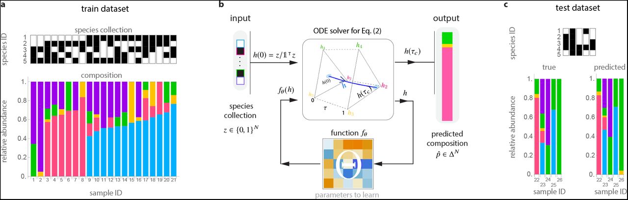
Here we show it is possible to predict the microbial composition from species assemblage without knowing the mechanistic details of the above processes. Our solution is a deep learning framework that learns the map φ directly from a dataset  of S samples, each of which is associated with a pair (z, p), see Fig. 1.

We illustrate this framework using experimental data from a pool of N = 5 bacterial species in Drosophila melangaster gut microbiota14: Lactobacillus plantarum (blue), Lactobacillus brevis (pink), Acetobacter pasteurianus (yellow), Acetobacter tropicalis (green), and Acetobacter orientalis (purple). a. We randomly split this dataset into training and test datasets:  and
and  , which contain 80% and 20% of the samples, respectively. Each dataset contains pairs (z, p) of the species assamblage z ∊ {0, 1}N (top) and composition p ∊ ΔN (bottom) from each sample. b. To predict compositions from species assamblages, our cNODE framework consists of a solver for the ODE shown in Eq. (2), together with a chosen parametrized function fθ . During training, the parameters θ are adjusted to learn to predict the composition
  of the species assamblage z ∊{0, 1}N in
  . c. After training, performance is evaluated by predicting the composition of never-seen-before species assamblages in the test dataset
  .
.
Conditions for predicting compositions from species assemblages
To ensure that the problem of learning φ from  is mathematically well-posed, we make the following assumptions. First, we assume that the species pool in the habitat has universal dynamics17, i.e., different local communities of this habitat can be described by the same population dynamics model with the same parameters. This assumption is necessary because, otherwise, the map φ simply does not exist, implying that predicting community compositions from species assemblages has to be done in a sample-specific manner, which is a daunting task. For in vitro communities, this assumption is satisfied if samples were collected from the same experiment or from multiple experiments but with very similar environmental conditions. For in vivo communities, empirical evidence indicates that the human gut and oral microbiota of healthy adults display very strong universal dynamics17. Second, we assume that the compositions of those collected samples represent steady states. This assumption is natural because for highly fluctuating microbial compositions the map φ is simply not well defined. We note that observational studies of host-associated microbial communities such as the human gut microbiota indicate that they remain close to stable steady states in the absence of drastic dietary change or antibiotic administrations15,18,19. Finally, we assume that for each species assemblage z ∊ {0, 1}N there is a unique steady-state composition p ∊ ΔN . In particular, this assumption requires that the true multi-stability does not exist for the species pool (or any subset of it) in this habitat. This assumption is required because, otherwise, the map φ is not injective and the prediction of community compositions becomes mathematically ill-defined. In practice, we expect that the above three assumptions can not be strictly satisfied. This means that any algorithm that predicts microbial compositions from species assemblages needs to be systematically tested to ensure its robustness against errors due to the violation of such approximations.
Limitations of traditional deep learning frameworks
Under the above assumptions, a straightforward approach to learning the map φ from  would be using deep neural networks20,21 such as a feedforward Residual Network22 (ResNet). As a very popular tool in image processing, ResNet is a cascade of L ≥ 1 hidden layers where the state hl ∊ ℝN of the l-th hidden layer satisfies hl = hl – 1 + fθ(hl – 1), l = 1, ⋯ , L, for some parametrized function fθ with parameters θ. These hidden layers are plugged to the input h0 = gin(z) and the output
  layers, where gin and gout are some functions. Crucially, for our problem, any architecture must satisfy two restrictions: (1) vector
  must be compositional (i.e.,
  ); and (2) the predicted relative abundance of any absent species must be identically zero (i.e., zi = 0 should imply that
  ). Simultaneously satisfying both restrictions requires that the output layer is a normalization of the form
  , and that fθ is a non-negative function (because hL ≥ 0 is required to ensure the normalization is correct). We found that it is possible to train such a ResNet for predicting compositions in simple cases like small in vitro communities (Supplementary Note S2.1). But for large in vivo communities like the human gut microbiota, ResNet does not perform very well (Supplementary Fig. S1). This is likely due to the normalization of the output layer, which challenges the training of neural networks because of vanishing gradients21. The vanishing gradient problem is often solved by using other normalization layers such as the softmax or sparsemax layers23. However, we cannot use these layers in our problem because they do not satisfy the second restriction. We also note that ResNet becomes a universal approximation only in the limit L → ∞, which again complicates the training24.

Vertical axis denotes prediction error.
A new deep learning framework
To overcome the limitations of traditional deep learning frameworks based on neural networks (such as ResNet) in predicting microbial compositions from species assemblages, we developed cNODE (compositional Neural Ordinary Differential Equation), see Fig. 1b. The cNODE framework is based on the notion of Neural Ordinary Differential Equations, which can be interpreted as a continuous limit of ResNet where the hidden layers h’s are replaced by an ordinary differential equation (ODE)25. In cNODE, an input species assemblage z ∊ {0, 1}N is first transformed into the initial condition  , where
  (left in Fig. 1b). This initial condition is used to solve the set of nonlinear ODEs

Here, the independent variable τ ≥ 0 represents a virtual “time”. The expression h ⊙ v is the entry-wise multiplication of the vectors h, v ∊ ℝN . The function fθ : ΔN → RN can be any continuous function parametrized by θ. For example, it can be the linear function fθ(h) = Θh with parameter matrix Θ ∊ ℝN×N (bottom in Fig. 1b), or a more complicated function represented by a feedforward deep neural network. Note that Eq. (2) can be considered as a very general form of the replicator equation —a canonical model in evolutionary game theory26— with fθ representing the fitness function. By choosing a final integration “time” τc > 0, Eq. (2) is numerically integrated to obtain the prediction  that is the output of cNODE (right in Fig. 1b). We choose τc = 1 without loss of generality, as τ in Eq. (2) can be rescaled by multiplying fθ by a constant. The cNODE thus implements the map
 taking an input species assemblage z to the predicted composition
  (see Supplementary Note S1 for implementation details). Note that Eq. (2) is key to cNODE because its architecture guarantees that the two restrictions imposed before are naturally satisfied. Namely,
  because the conditions h(0) ∊ ΔN and
  imply that h(τ) ∊ ΔN for all τ ≥ 0. Additionally, zi = 0 implies
  because h(0) and z have the same zero pattern, and the right-hand side of Eq. (2) is entry-wise multiplied by h.
We train cNODE by adjusting the parameters θ to approximate φ with  . To do this, we first choose a distance or dissimilarity function d(p, q) to quantify how dissimilar are two compositions p, q ∊ ΔN . One can use any Minkowski distance or dissimilarity function. In the rest of this paper, we choose the Bray-Curtis27 dissimilarity to present our results. Specifically, for a dataset
  , we use the loss function

Second, we randomly split the dataset  into training
  and test
  datasets. Next, we choose an adequate functional form for fθ. In our experiments, we found that the linear function fθ(h) = Θh, Θ ∊ ℝN × N , provides accurate predictions for the composition of in silico, in vitro, and in vivo communities. Note that, despite fθ is linear, the map
  is nonlinear because it is the solution of the nonlinear ODE of Eq. (2). Finally, we adjust the parameters θ by minimizing Eq. (4) on
  using a gradient-based meta-learning algorithm28. This learning algorithm enhances the generalizability of cNODE (Supplementary Note S1.2 and Supplementary Fig. S1). Once trained, we calculate cNODE’s test prediction error
  that quantifies cNODE’s performance in predicting the compositions of never-seen-before species assemblages. Test prediction errors could be due to a poor adjustment of the parameters (i.e., inaccurate prediction of the training set), low ability to generalize (i.e., inaccurate predictions of the test dataset), or violations of our three assumptions (universal dynamics, steady-state samples, no true multi-stability).
Fig. 1 demonstrates the application of cNODE to the fly gut microbiome samples collected in an experimental study14. In this study, germ-free flies (Drosophila melanogaster) were colonized with all possible combinations of five core species of fly gut bacteria, i.e., Lactobacillus plantarum (species-1), Lactobacillus brevis (species-2), Acetobacter pasteurianus (species-3), Acetobacter tropicalis (species-4), and Acetobacter orientalis (species-5). The dataset contains 41 replicates for the composition of each of the 2N - 1 = 31 local communities with different species assamblages. To apply cNODE, we aggregated all replicates and calculated their average composition, resulting in one “representative” sample per species assamblage (Supplementary Note S4). We also excluded the trivial samples with a single species, resulting in S = 26 samples. We trained cNODE by randomly choosing 21 of those samples (80%) as the training dataset (Fig. 1a). Once trained, cNODE accurately predicts microbial compositions in the test dataset of 5 species assemblages (Fig. 1c). For example, cNODE predicts that in the community with only species 3 and 4 present, species 3 will become nearly extinct, which agrees well with the experimental result (sample 26 in Fig. 1c).
Results
In silico validation of cNODE
To systematically evaluate the performance cNODE, we generated in silico data for pools of N = 100 species with population dynamics given by the classical Generalized Lotka-Volterra (GLV) model29

Above, xi(t) denotes the abundance of the i-th species at time t ≥ 0. The GLV model has as parameters the interaction matrix A = (aij) ∊ ℝNxN, and the intrinsic growth-rate vector r = (ri) ∊ ℝN . Here, aij denotes the inter- (if j ≠ i) or intra- (if j = i) species interaction strength of species j to the per-capita growth rate of species i. The parameter ri is the intrinsic growth rate of species i. Recall that the interaction matrix A determines the ecological network  underlying the species pool. Namely, this network has one node per species and edges
  . The connectivity C ∈ [0, 1] of this network is the proportion of edges it has compared to the N2 edges in a complete network. Despite its simplicity, the GLV model has been successfully applied to describe the population dynamics of microbial communities in diverse environments, from the soil30 and lakes31 to the human gut32,33. To validate cNODE, we generated synthetic microbiome samples as steady-state compositions of GLV models with random parameters by choosing aij ~ Bernoulli(C)Normal(0, σ) if i ≠ j, aii = −1, and ri ~ Uniform[0, 1], for different values of connectivity C and characteristic inter-species interaction strength σ > 0 (Supplementary Note S3).
Figure 2a shows the prediction error in synthetic training and test datasets, each of which has N samples generated by the GLV model of N species, with σ = 0.5 and different values of C. The prediction error in the training set,  , keeps decreasing with the increasing number of training epochs, especially for high C values (as shown in dashed and dotted cyan lines in Fig. 2a). Interestingly, the prediction error in the test dataset,
  , reaches a plateau after enough number of training epochs regardless of the C values (see solid, dashed and dotted yellows lines in Fig. 2a), which is a clear evidence of an adequate training of cNODE with low overfitting. Note that the plateau of
  increases with C. We confirm this result in datasets with different sizes of the training dataset (Fig. 2b). Moreover, we found that the plateau increases with increasing characteristic interaction strength σ (Fig. 2c). Fortunately, the increase of
  (due to increasing C or σ) can be compensated by increasing the sample size of the training set
  . Indeed, as shown in Fig. 2b,c,
  decreases with increasing
  .
.

Results are for synthetic communities of N = 100 species generated by the with Generalized Lotka-Volterra model (panels a-e) or a population dynamics model with nonlinear functional responses (panel f). a. Training cNODE with N samples obtained from GLV models with connectivity C = 0.1 (solid), C = 0.15 (dashed), C = 0.2 (dotted). b. Performance of cNODE for GLV datasets with C = 0.5 and different interaction strengths σ. c. Performance of cNODE for GLV datasets with σ = 0.5 and different connectivity C. d. Performance of cNODE for GLV datasets with non-universal dynamics, quantified by the value of η. For all datasets, σ = 0.1 and C = 0.5. e. Performance of cNODE for GLV datasets with measurement errors quantified by ɛ. For all datasets, σ = 0.1 and C = 0.5. f. Performance of cNODE for synthetic datasets with multiple interior equilibria, quantified by the probability μ ∊ [0, 1] of finding multiple equilibria. For all datasets, C = 0.5, σ = 0.1. In panels b-f, thin lines represent the prediction errors for ten validations of training cNODE with a different dataset. Mean errors are shown in thick lines.
To systematically evaluate the robustness of cNODE against violation of its three key assumptions, we performed three types of validations. In the first validation, we generated datasets that violate the assumption of universal dynamics. For this, given a “base” GLV model with parameters (A, r), we consider two forms of universality loss (Supplementary Note S3). First, samples are generated using a GLV with the same ecological network but with those non-zero interaction strengths aij replaced by aij + Normal(0, η), where η > 0 characterizes the changes in the typical interaction strength. Second, samples are generated using a GLV with slightly different ecological networks obtained by randomly rewiring a proportion ρ ∈ [0, 1] of their edges. We find that cNODE is robust to both forms of universality loss as its asymptotic prediction error changes continuously, maintaining a reasonably low prediction error up to η = 0.4 and ρ = 0.1 (Fig. 2d and Supplementary Fig. S2).

Vertical axis denotes prediction error.

Prediction errors of Maynard et al.’s method40 and cNODE.
For an in silico dataset of N = 5 species with universal dynamics and different typical interaction strength. Circles denote mean error for 10 repetitions, and gray shadows indicate standard deviation of the mean. a. Train dataset. b. Test dataset.
In the second validation, we evaluated the robustness of cNODE against measurement noises in the relative abundance of species. For this, for each sample, we first change the relative abundance of the i-th species from pi to max{0, pi + Normal(0, ε)}, where ε ≥ 0 characterizes the measurement noise intensity. Then, we normalize the vector p to ensure it is still compositional, i.e., p ∈ ΔN. Due to the measurement noise, some species that were absent may be measured as present, and vice-versa. In this case, we find that cNODE performs adequately up to ε = 0.025 (Fig. 2f)
In the third validation, we generated datasets with true multi-stability by simulating a population dynamics model with nonlinear functional responses (Supplementary Notes S3). For each species collection, these functional responses generate two interior equilibria in different “regimes”: one regime with low biomass, and the other regime with high biomass. We then train cNODE with datasets obtained by choosing a fraction(1 − μ) of samples from the first regime, and the rest from the second regime. We find that cNODE is robust enough to provide reasonable predictions up to μ = 0.2 (Fig. 2d).
Evaluation of cNODE using real data
We evaluated cNODE using six microbiome datasets of different habitats (Supplementary Note S4). The first dataset consists of S = 275 samples34 of the ocean microbiome at phylum taxonomic level, resulting in N = 73 different taxa. The second dataset consists of S = 26 in vivo samples of Drosophila melanogaster gut microbiota of N = 5 species14, as described in Fig. 1. The third dataset has S = 93 samples of in vitro communities of N = 8 soil bacterial species12. The fourth dataset contains S = 113 samples of the Central Park soil microbiome13 at the phylum level (N = 36 phyla). The fifth dataset contains S = 150 samples of the human oral microbiome from the Human Microbiome Project15 (HMP) at the genus level (N = 73 genera). The final dataset has S = 106 samples of the human gut microbiome from HMP at the genus level (N = 58 genera).
To evaluate cNODE, we performed the leave-one-out cross-validation on each dataset. The median test prediction errors were 0.06, 0.066, 0.079, 0.107, 0.211 and 0.242 for the six datasets, respectively (Fig. 3a). To understand the meaning of these errors, for each dataset we inspected five pairs  corresponding to the observed and the predicted compositions of five samples. We chose the five samples based on their test prediction error. Specifically, we selected those samples with the minimal error, close to the first quartile, closer to the median, closer to the third quartile, and with the maximal error (columns in Fig. 3b-g, from left to right). We found that samples with errors below the third quartile provide acceptable predictions (left three columns in Fig. 3b-g), while samples with errors close to the third quartile or with the maximal error do demonstrate salient differences between the observed and predicted compositions (right two columns in Fig. 3b-g). Note that in the sample with largest error of the human gut dataset (Fig. 3g, rightmost column), the observed composition is dominated by Provotella (pink) while the predicted sample is dominated by Bacteroides (blue). This drastic difference is likely due to different dietary patterns35.

a. Boxplots with the prediction error obtained from a leave-one-out crossvalidation of each dataset. b-g: For each dataset, we show true and predicted samples corresponding to the minimal prediction error, closer to the first quartile, median, closer to the third quartile, maximum prediction error (including outliers). Note all shown in panels b-g predictions are out-of-sample predictions.
Discussion
cNODE is a deep learning framework to predict microbial compositions from species assemblages. We validated its performance using in silico, in vitro, and in vivo microbial communities. Several methods have been developed for predicting species abundances in microbial communities by modeling their population dynamics12,32,36,37, but these methods typically require high-quality time-series data of absolute abundances that are difficult to obtain for large in vivo microbial communities. cNODE circumvents the need of absolute abundances or time-series data. The price to pay is that the trained function fθ cannot be directly interpreted because the lack of identifiability inherent to compositional data38,39. We also note a recent statistical method to predict coexistence of ecological communities40, but this method also requires absolute abundance measurements. cNODE can outperform this statistical method despite using only relative abundances (Supplementary Note S6). See also Supplementary Note S5 for a discussion of how our framework compares to other related works.
Deep learning techniques are actively applied to microbiome research41–49 such as for classifying samples that shifted to a diseased state50, predicting infection complications in immunocompromised patients51, or predicting the temporal or spatial evolution of certain species collection52,53. However, to the best of our knowledge, the potential of deep learning for predicting the effect of changing species collection was not explored nor validated before. Our proposed framework based the notion of neural ODE is a baseline which could be improved by incorporating additional information. For example, incorporating available environmental information such as pH, temperature, age, BMI and diet of the host, could enhance the prediction accuracy. This would help to predict the species present in different environments. Adding “hidden variables” such as the unmeasured total biomass or unmeasured resources to our ODE will enhance the expressivity of the cNODE54,55, but this may result in a more challenging training. Finally, if available, knowledge of the genetic similarity between species can be leveraged into the loss function by using the phylogenetic Wasserstein distance56 that provides a well-defined gradientt57.
Our framework does have limitations. For example, it cannot accurately predict the abundance of taxa that have never been observed in the training dataset. Also, a limitation of our current architecture is that it assumes that true multistability does not exist —namely, a community with a given species assemblage permits only one stable steady-state, where each species in the collection has a positive abundance. For complex microbial communities such as the human gut microbiota, the highly personalized species collections makes it very difficult to decide if true multistability exists or not. Our framework could be extended to handle multi-stability by predicting a probability density function for the abundance of each species. In such a case, true multistability would correspond to predicting a multimodal density function.
We anticipate that a useful application of our framework is to predict if by adding some species collection to a local community we can bring the abundance of target species below the practical extinction threshold. Thus, given a local community containing the target (and potentially pathogenic) species, we could use a greedy optimization algorithm to identify a minimal collection of species to add such that our architecture predicts that they will decolonize the target species.
Competing financial interests
The authors declare no competing financial interests.
Author contributions
M.T.A. and Y.-Y. L. conceived and designed the project. S.M.M. did the numerical analysis. S.M.M. and X.-W.W. performed the real data analysis. All authors analyzed the results. M.T.A. and Y.-Y.L. wrote the manuscript. S.M.M. and X.-W.W. edited the manuscript.
Data accessibility
The data and code used in this work are available from the corresponding authors upon reasonable request.
Supplementary Notes
S1. Implementation of the compositional Neural Ordinary Differential Equation
S1.1 Flux implementation of cNODE
We implemented cNODE using Flux58, a library for machine learning in the Julia programming language with support for Neural Ordinary Differential Equations25. A complete implementation of cNODE is given in the file cNODE.jl.
Our implementation is based on a structure called FitnessLayer that contains cNODE’s parameter Θ ∈ ℝN×N. This parameter is initialized using the Xavier’s method59. When evaluated in a composition p, the FitnessLayer computes first fθ(p) = Θp. More complex functions fθ can be easily incorporated in the code. Finally, the structure uses fθ to calculate the right-hand side of the ODE in Eq. (2).
To predict the composition  associated with a species collection z ∈ {0, 1}N, cN-ODE numerically solves such an the ODE in Eq.(2). In Flux, this is automated by the function neural_ode, which constructs the cNODE by building a NODE with the dynamics specified by the FitnessLayer.
The dynamics is numerically integrated over the interval τ ∈ [0, τc] using the Tsit5 method60, which is the default integration method for nonsgif ODEs in Julia. We choose τc = 1 without loss of generality, as τ in Eq. (2) can be rescaled by multiplying fθ by a constant. After integration, the final value at time τ = 1.0 is returned as the prediction of cNODE.
The loss function calculates the average Bray-Curtis dissimilarity between there true composition p ∈ ΔN and the prediction  generated by cNODE.
S1.2 Training cNODE
To train cNODE, we adjust the parameters θ to minimize the loss over the training set. We experimented with two training algorithms:
The ADAM algorithm61. ADAM is a widely used gradient-based stochastic optimization algorithm that often compares favorably to other gradient optimization algorithms62. We refer to [61, 62] for additional details.
ADAM plus a first-order gradient-based meta-learning algorithm based on Reptile28. In the meta-learning framework, lets consider a set
 of different tasks that the network needs to perform, such as learning to predict in different datasets. Reptile works by sampling some task , training on it to obtain the weights , and then updating the initial weights 0 towards.


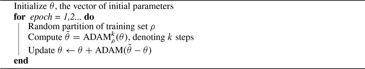
To train cNODE, we used ADAM plus Reptile training28. More precisely, we defined each task as a random partition of the training set in mini-batches. In this way, training enhances cNODE’s generalizing ability from the predictions regardless of any specific partition or any sequence order of mini-batches. The algorithm we used is described below:

ADAM + Reptile for cNODE
Our implementation in the Julia language of the above algorithm is based on the model zoo of the library Flux63.
S2. Comparison of two deep learning frameworks in predicting microbiome compositions
S2.1 A ResNet architecture for predicting microbiome compositions
We tested the performance the classical ResNet architecture25 for predicting microbiome compositions. More precisely, we used the input layer
 where W0 ∈ ℝN×N and b0 ∈ ℝN are parameters to adjust. We used L = 3 hidden layers of the form:
 where Wl ∈ ℝN×N and bl ∈ ℝN are parameters to adjust. Finally, the output layer takes the form

A Flux implementation of this ResNet can be found in the file ResNet.jl. We trained this ResNet architecture using the two methods described in S1.2.
S2.2 Performance comparison
We compared the performance of cNODE and ResNet architecture for predicting the composition of four out of six real microbiome datasets described in Supplementary Note S4. These datasets contain a small set of species (between 5 and 58) and samples (between 26 and 113), allowing us to make computationally expensive leave-one-out cross validation analysis. Here, we also compared the effect of training both architectures with ADAM, and with ADAM plus the Reptile like metalearning algorithms.
To perform the comparison we used a leave-one-out cross validation on each of the four datasets (Supplementary Fig. S1). From these results, some remarks are in order:
For both in-vivo datasets, cNODE trained with Reptile outperforms all other algorithms.
The ResNet architecture trained using only ADAM can provide reasonably accurate prediction for simple small species collections (i.e., for the N = 5 species in Drosophila gut and the N = 8 species in the soil in-vitro community).
For cNODE, training using the Reptile metalearning algorithm decreases the prediction error in the test dataset. Interestingly, using Reptile does not alway decreases the prediction error in the train dataset. Therefore, the Reptile metalearning algorithm is performing as desired to enhance the generalizing ability of cNODE.
For ResNet, training with the Reptile metalearning algorithm can increase the prediction errors in both the training and test datasets when compared to training only with ADAM.
The ResNet architecture exhibits a higher variability in the training set when compared to cNODE. This suggests that the performance of ResNet is significantly influenced by the initialization parameters. In particular, training a ResNet with Reptile can significantly increase the variability of prediction errors (see, e.g., the soil in vitro dataset).
Overall, the above remarks indicate that cNODE training with Reptile outperforms the other architectures when predicting complex microbial communities like human gut microbiota or in vivo soil communities.
S3. Population dynamics for the in silico validations
We generated in-silico species pools using the Generalized Lotka-Volterra (GLV) equations, a classical population dynamics model successfully applied to diverse microbial communities, from soils30 and cheese36, to the human body32,33. The GLV model takes the form
 where x(t) = (x1(t), … , xN (t))⊤ ∈ ℝ≥0 and xi (t) denotes the absolute abundance of species i at time t . Above, x ⊙ ν is the entry-wise multiplication of vectors x, ν ∈ ℝN . The GLV model has two parameters: the interaction matrix of the species pool A = (aij) ∈ ℝN×N, and the intrinsic growth-rate of the species r = (ri) ∈ ℝN. In particular, the j-th species has a positive impact on the i-th species if aij > 0, a negative impact if aij < 0, and no impact if aij = 0. Recall also that the interaction matrix determines the underlying ecological network
  of the species pool. This network has one vertex associated to each species and an edge
  .
.
To generate the relative abundance vector p ∈ ΔN corresponding to a local community with species collection z ∈ {0,1}N, we follow four steps:
Set the parameters (A, r).
Set the initial abundance of species
as
for i = 1, ⋯ , N.Numerically integrate Eq. (S1) with initial condition xθ until the system reaches a steady-state abundance
. For the results presented in our paper, we choose a final integration time tf = 1000.Compute the relative abundance vector p = (p1, ⋯ , pN)T ∈ ΔN as
.


Using the above procedure, we generated a dataset  by randomly sampling species collections z ∈ {0, 1}N and calculating the corresponding
  . Below we detail the construction of the three types of datasets used in the Main Text.
S3.1 Generating datasets with universal dynamics
To generate a dataset with universal dynamics, we considered that all species collections have the same parameters (A, r). These parameters were generated as follows. The interaction matrix A of the community is obtained as the adjacency matrix of a directed weighted Erdös-Rényi random network with connectivity C ∈ [0, 1]. The edge-weights were chosen from a Normal distribution with zero mean and variance σ2 , where σ > 0 represents the “characteristic” inter-species interaction strength. The intrinsic growth ri is chosen uniformly at random from the interval [0, 1].
S3.2 Generating datasets with non-universal dynamics
To generate a dataset with non-universal dynamics, we considered two possible sources for non-universality. First, the mechanisms of interaction between species may differ across local communities. In Eq. (S1), this translates as using different parameters aij for each non-zero interaction in different local communities. Thus, in this case we replaced each aij ≠ 0 by aij + ηNormal(0, 1), where η > 0 quantifies the changes in the typical interaction strength, and hence the “loss” of universality in this case.
Second, we considered that each local community may have a different ecological network. To model this case, we considered that the ecological network of each local community is obtained by randomly rewiring a proportion ρ ∈ [0, 1] of the edges of a baseline ecological network  , thus shuffling a proportion of entries of the associated A matrix. Since ρ = 0 corresponds to universal dynamics, the magnitude of ρ quantifies the “loss” of universality in this case.
S3.3 Adding measurement noise to a dataset
For a pair (z, p) in a dataset  , we added noise by replacing pi by first adding a small noise wi = max{0, pi + εNormal(0, 1)}, and then normalizing to obtain the noisy measurement pi ← wi/∑j wj. Here, the parameter ε > 0 controls the measurement noise intensity.
S3.4 Generating datasets with multi-stability
To generate a dataset with true multi-stability, we calculated the steady-states from a population dynamics model with the following non-linear functional response:
 where h denotes the handling time.
To generate steady-states with multi-stability, we first select a GLV model with a linear functional response (Eq. S1) and universal dynamics (Supplementary Notes S3), and compute the steady-state  . Note that the steady-state abundances satisfies the equation

The steady-states of Eq.(S2) satisfies the equation
 so that we substitute Eq.S3 in Eq.S4 and solve for xj the following quadratic equation:
 for all j, and then we compute the relative abundance vector p = (p1, … pN)T ∈ ΔN as
  To ensure that there are two real solutions for xj, we chose
  for some k.
The two steady-state abundances corresponds to a high and low total biomass regimes, respectively. To build the datasets, we chose a fraction (1-μ) from the first regime, and the rest from the second.
S4. Description of the experimental datasets
S4.1 In-vivo drosophila core gut microbiome
The drosophila dataset14 contains the absolute abundance of the five species in each possible local community with different species collection. See Supplementary Table S1 for species IDs. There is five replicates for each of those species collections. We averaged those five replicates, discarded samples with a single species, and obtained the relative abundance of each of the remaining samples. This yielded 31 samples with different species collection.
Species IDs Drosophila gut microbiota.
S4.2 In-vitro soil community
This laboratory community of N = 8 heterotrophic soil-dwelling bacterial species12 described in Table S2. The available dataset contains 98 samples, including all solos, all duos, some trios, one septet and one octet.
Species IDs the in-vitro soil community.
S4.3 In-vivo soil microbiome
The soil dataset consists of soil microbiome across Central Park in New York City consist of 1160 samples. This data set is 16S rRNA gene-based with variable region V4. The data is available at https://qiita.ucsd.edu/ under study ID 2140 and the detailed description of this data set can be found in Ref. [13]. We used the function summarize_taxa.py QIIME 1 to summarize taxa to different taxonomic levels with defaults options. Supplementary Table S3 provides the IDs associated to each phylumm.
S4.4 Human gut microbiome
A 16S rRNA gene-based data set from variable regions V3 to V5. The data are available at http://www.hmpdacc.org/HMQCP/. We selected the samples from the stool body site. For multiple samples from the same subject, we only keep one single sample of that subject. To guarantee the model can be trained sufficiently, we summarized the taxa into the genus level and removed the genus with fewer than 50 reads. See also Supplementary Table S4 for genus ID.
Phylum IDs for soil dataset.
Genus IDs for the human gut microbiota dataset.
S5. Related work
Here we describe related methods, emphasizing some key differences with respect to our framework.
Abundance prediction based on inferred population dynamics. A classical method to predict species abundance in microbial ecosystems is modeling their population dynamics12,32,33,36,37. Typically, the model is a set of parametrized ODEs —such as the Generalized Lotka-Volterra equations— describing the changes over time in the absolute abundances of a set of species. The model is fitted to available temporal data of absolute abundance to infer parameters, such as intrinsic growth rates, inter-species interaction strengths, etc. Then, to predict the abundance of certain species collection, the fitted ODE model is solved starting from suitable initial condition. However, applying this method for large microbial communities like the human gut is challenging if not impossible because: 1) the absence of high-quality temporal data; and 2) typically only relative abundance of species are measured. Furthermore, because the very broad population dynamics that ecosystems display even at the scale of two species64, it is always very challenging to choose an adequate parametrized ODE model for the population dynamics of the community.
Predictions based on neural networks methods. Larsen et al.52 employed an artificial neural network to predict the temporal evolution of the composition of bacterial communities with a constant species collection. More precisely, they developed a bioclimatic model of relative microbial abundance that specifically incorporates interactions between biological units. They modeled the complex interactions between microbial taxa and their environment as an artificial neural network (ANN). This method is based on two key assumptions: (1) community patterns share mathematically describable relationships with environmental conditions; and (2) the ecosystem maintains a persistent microbial community. Note that the second assumption implies that this method can not be used to predict the impact of changing the species collections. Compared to method based on inferring population dynamics, this method has the advantage of not requiring to specify any model for the community dynamics. However, in contrast to our framework, this method cannot predict the effect of changing the species collection.
Similarly, the recent work of Zhou et al.53 uses a neural network to predict the temporal and spatial evolution of the composition of microbial communities with a constant species collection. More precisely, the authors formulated the prediction of microbial communities at unsampled locations as a multi-label classification task, where each location is considered as an instance and each label represents a microbe species. Based on a set of heterogeneous features extracted from the urban environment, they aimed to predict the presence or absence of a list of microbes species at a nearby location. Note, however, that this method cannot be immediately used to predict the effect of changing the species collection.
Predictions based on statistical methods. Recently, Maynard et al.40 proposed a statistical method to predict species abundances from species collections. More precisely, based on measuring the absolute abundance of species at some steady-states of the ecosystem, this method assumes a linear model to predict all other steady-states. For the method to be applicable, it requires that the following assumptions are satisfied: (1) each species must be present in at least n distinct endpoints, not counting replicates; (2) each species must co-occur with each other species in at least one endpoint (that is, for every pair of species i and j , there must be some endpoint where i and j co-occur, possibly along with other species); and (3) for each i there must exist a perfect matching between the n species and the endpoints in which they co-occur with i . As explained in the original manuscript40, conditions (1) and (2) above requires that “coexistence among species must be reasonably widespread for [these] conditions to hold.” This method may be challenging to apply for microbial communities because it requires measuring absolute abundances. Furthermore, because microbial communities tend to have nonlinear behaviors even at the scale of two species64,65, the implicit assumption of linearity may fail to be satisfied. Finally, we note that cNODE does not require any of the above three assumptions to be applicable, although its prediction accuracy may be influenced by them.
Similarly, Tung et al.66 use a linear regression method to predict species compositions from information of social networks of individuals. More precisely, the authors fit a classical linear mixed model to predict the relative abundance of species in a sample based on the following predictors: social group membership, age, sex, and read depth. We note here that the predictors in this approach are completely different than the predictors used in cNODE (i.e., it only uses species collections), and thus are not comparable.
S6. Comparing cNODE with Maynard et al.’s method
Here we compare the performance of cNODE with the method of Maynard et al. for predicting endpoints40. This last method is described with details in item 3 of Supplementary Note S5.
To perform the comparison, we generated in silico datasets of N = 5 species with Generalized Lotka-Volterra dynamics. More precisely, we generated datasets with universal dynamics, maintaining the connectivity C = 0.5 constant and changing the typical interaction strength as σ ∊ {0.1, 0.2, 0.3, 0.4}. For each value of a, we generated 10 datasets containing all S = 25 − 1 samples with different species collections following the simulation method described in Supplementary Note S3. We repeated this simulation method three times, obtaining three repetitions for the abundance of each species collections that can be used in Maynard’s method. Additionally, because Maynard’s method requires absolute abundances, we kept in the datasets both the absolute abundance and relative abundance of each steady-state that is reached. Using these datasets, we constructed training datasets by randomly choosing 70% of the samples, and the rest of the samples as test datasets.
To adjust Maynard’s method we used the default parameters that were selected for N = 4 species. After this, we obtained the corresponding absolute abundance predictions of the test dataset. Finally, to allow a comparison with cNODE that predicts relative abundances, we transformed each predicted absolute abundance into a predicted relative abundance, and then calculated the prediction error using the Bray-Curtis dissimilarity.
For cNODE, we used the exact same training dataset as for Maynard’s method, the only difference being that we trained cNODE with relative abundances. We choose a inner learning rate of 0.001, an outer learning rate of 0.005, and trained cNODE for 500 epochs using mini batches of 5 samples. We then calculated the prediction error in the test dataset using the Bray-Curtis dissimilarity. We emphasize that cNODE uses less information that Maynard’s method, in the sense that the total biomass of each sample is unknown in this case.
The results of the comparison of Maynard’s method and cNODE are shown in Fig. S3. We find that, for the above conditions used to construct the datasets, cNODE outperforms Maynard’s method in both the training and test datasets. Crucially, note that cNODE was trained using only relative abundance measurements. We do not claim this results holds for all datasets, as there might be cases where the assumptions required by Maynard’s method are exactly satisfied but none of the assumptions of cNODE are satisfied.
Acknowledgments
M.T.A. gratefully acknowledges the financial support from CONACyT project A1-S-13909, México. Y.-Y.L. acknowledges the funding support from National Institutes of Health (R01AI141529, R01HD093761, RF1AG067744 , UH3OD023268, U19AI095219, and U01HL089856).


