

Abstract
Vigilance and wakefulness modulate estimates of functional connectivity, and, if unaccounted for, they can become a substantial confound in resting-state fMRI. Unfortunately, wakefulness is rarely monitored due to the need for additional concurrent recordings (e.g., eye tracking, EEG). Recent work has shown that strong fluctuations around 0.05Hz, hypothesized to be CSF inflow, appear in the fourth ventricle (FV) when subjects fall asleep. The analysis of these fluctuations could provide an easy way to evaluate wakefulness in fMRI-only data. Here we evaluate this possibility using the 7T resting-state sample from the Human Connectome Project. Our results confirm the presence of those fluctuations in the HCP sample despite this data having relatively small inflow weighting. Moreover, we show that fluctuations of a similar frequency appear in large portions of grey matter with different temporal delays, and that they can substantially influence estimates of functional connectivity. Finally, we demonstrate that the temporal evolution of this signal cannot only help us reproduce previously reported overall sleep patterns in resting-state data, but also predict individual periods of eye closure with 70% accuracy, matching predictions attainable using the amplitude of the global signal (a common fMRI marker of arousal). In summary, our results demonstrate the ubiquitous presence of this signal in a large, publicly available, fMRI sample, its value as a marker of arousal in absence of a better metric, its relationship to the global signal, and its potential nuisance effects on functional connectivity estimates when ignored.
Introduction
Vigilance and wakefulness modulate estimates of functional connectivity, and, if unaccounted for, they can become a substantial confound (Haimovici et al., 2017; Laumann et al., 2016; Tagliazucchi and Laufs, 2014). This is particularly important for clinical studies where one can expect differences in vigilance/wakefulness across populations. Similarly, whether subjects keep their eyes open or closed during a given scan can also influence functional connectivity estimates (Agcaoglu et al., 2019; Dijk et al., 2010; Patriat et al., 2013). Despite such evidence, instructions regarding eye closure are not consistent across resting-state studies (Waheed et al., 2016). Moreover, eye closures (and wakefulness levels) are rarely monitored, because doing so would require some form of concurrent recordings such as eye tracking (ET; (Chang et al., 2016; Falahpour et al., 2018; Poudel et al., 2014)) or electro-encephalography (EEG; (Larson-Prior et al., 2011, 2009)). Such concurrent acquisitions are not common practice in resting-state research, and the effects of fluctuations in wakefulness (or subject’s lack of compliance with keeping eyes open) are often ignored. Prior research has demonstrated that subjects have a propensity to fall asleep during resting-state scans (Allen et al., 2014; Tagliazucchi and Laufs, 2014), and that fluctuations in vigilance are to be expected (Chang et al., 2016; Liu and Falahpour, 2020). It is important to find ways to determine the occurrence of these events when no concurrent measures are available. This capability would not only help in future study design but may be used to assess the degree to which vigilance fluctuations have confounded previously acquired fMRI-only datasets.
Previous work has shown that it is possible to predict sleep stages (Altmann et al., 2016; Enzo Tagliazucchi et al., 2012), and vigilance levels (Falahpour et al., 2018) relying solely on fMRI data. For example, Tagliazucchi and colleagues (2012) showed how it is possible to predict sleep stages with up to 80% prediction accuracy using dynamic traces of functional connectivity among 22 brain regions (20 cortical + 2 subthalamic nuclei) as inputs to a hierarchical tree of support linear vector machines. Similarly, significant correlation has been previously reported between fluctuations in vigilance based on EEG measures and both the global fMRI signal (Wong et al., 2013) and the average signal within a data-driven spatial template of pertinent regions (Falahpour et al., 2018). Yet, these methods have not been widely adopted by the community, either because pre-trained classifier approaches are complex (Altmann et al., 2016; E Tagliazucchi et al., 2012), or because their efficacy has only been demonstrated in small samples (e.g., 10 participants for (Falahpour et al., 2018)). It is unknown how well they may generalize beyond these small samples. Motivated by the technical need for simpler, more easily generalizable methods, and by recent work (Fultz et al., 2019) reporting that subject’s descent into sleep is accompanied by the appearance of ultra-slow (i.e., around 0.05Hz), inflow-related fluctuations in the fourth ventricle (FV), we aimed to study the value of those fluctuations as a marker of arousal in fMRI-only datasets, and their influence on functional connectivity.
We perform this evaluation in several steps. First, we study if the above-mentioned sleep-related fluctuations can be observed in an fMRI dataset (HCP dataset) not necessarily optimized to capture inflow effects. This is a key first step because the original observation of this phenomenon by Fultz and colleagues relied on data acquired at a very short TR (367ms) and with the lower boundary of the imaging field of view sitting over the FV; both set this way to maximize sensitivity to inflow effects in inferior ventricular regions. This was a logical decision for their work based on the hypothesized origin of this signal—namely inflow effects due to reversal of CSF flow during sleep (Fultz et al., 2019; Grubb and Lauritzen, 2019). Yet, most fMRI data, including the HCP 7T data used here, are not acquired with a short TR to maximize inflow effects (Gao and Liu, 2012). Once our ability to detect this signal in the HCP dataset was confirmed, we studied in detail the locations and timings of these sleep-related fluctuations. The presence of the fluctuations in superior ventricular regions would facilitate detection and modeling in datasets with limited fields of view that do not include the FV. Similarly, the spatiotemporal profile of these fluctuations in grey matter determines how they influence estimates of functional connectivity (which we also assess here). Finally, we study to what extent increases in spectral power around 0.05Hz in the FV can help us predict long periods of eye closure associated with descent into sleep. We compare the efficacy of this FV signal as a marker of arousal to that of the amplitude of the global signal; which is known to negatively correlate with vigilance (Liu et al., 2017; Liu and Falahpour, 2020; Wong et al., 2013) and to increase during sleep (Horovitz et al., 2008; Larson-Prior et al., 2009).
Our results confirm the presence in the HCP 7T resting-state dataset of these signals in both the FV and in superior ventricular regions. We also show that fluctuations of a similar frequency appear in large portions of grey matter with different temporal delays, and that they can substantially influence estimates of functional connectivity. Next, we demonstrate that the temporal evolution of the spectral density of FV correlates with overall sleep patterns detected in other resting state samples. Finally, using the FV fluctuations, we predict long periods of eye closure with similar accuracy to the amplitude of the global signal. All these results highlight the informative, but also nuisance, value of this easily computable FV signal.
Methods
Data
This study was conducted using a subset of the Human Connectome Project (HCP) dataset (Essen et al., 2013). We used the resting-state scans acquired on the 7T system and made publicly available as part of the 1200 Data Release (March 2018). This data subset consists of 723 different resting-state scans (15 mins each) acquired on a group of 184 subjects. This data was selected because concurrent eye pupil traces are available as part of the data release, and because the relatively short TR (1s), multi-band protocol, and high field (7T) allows for potential residual inflow effects in the FV. Basic scanning parameters for this data are TR=1s, TE=22.2ms, FA=45°, Voxel Resolution=1.6×1.6×1.6mm3, Multiband Factor=5, GRAPPA=2. Additional details can be found on the Reference Manual for the 1200 HCP Release available online at https://www.humanconnectome.org/storage/app/media/documentation/s1200/HCP_S1200_Release_Reference_Manual.pdf.
For this work, we downloaded the resting-state data following minimal pre-processing (Glasser et al., 2013), which includes distortion correction, motion correction and spatial normalization to the MNI template space. In addition, we also downloaded the T1 weighted images (for visualization purposes), Freesurfer (Fischl, 2012) anatomical parcellations (for ROI selection), and eye tracking recordings (to be used as a proxy for fluctuations in wakefulness).
Only 404 scans from the 723 initially available were considered in this study. Table 1 lists the criteria for scan exclusion and the number of scans removed due to each criterium.
Criteria for elimination of individual scans from the final sample entering all analyses.
Eye Tracking
Eye Tracking Data Pre-processing
First, we removed pupil size samples that fell outside the temporal span of each fMRI scan to achieve temporal synchronization between the fMRI and eye tracking data. Second, we removed blink artifacts. Any period of missing pupil size data shorter than 1 second was considered a blink, and data within that period was linearly interpolated between the onset and offset of the blink. Periods of missing pupil size data longer than one second are considered eye closures and were not interpolated. Third, we observed short bursts (< 1ms) of pupil size data scattered within periods of eye closure. Those bursts were removed to ensure the continuity and correct identification of long periods of eye closure. Forth, pupil size traces acquired at 500Hz (which is the case for 68 scans) were linearly upsampled to 1KHz to match the rest of the sample. Fifth, pupil size traces were temporally smoothed using a 200ms Hanning window. Sixth, pupil size traces were downsampled to 1Hz in order to match the temporal resolution of the fMRI data. Once pupil size traces were at the same temporal resolution as the fMRI data, we perform two additional operations: a) we removed the first 10 seconds of data (to match pre-processing of fMRI data outlined below) and b) we removed isolated single pupil size samples surrounded by missing data (Suppl. Figure 1.A), as well as interpolated isolated missing samples surrounded by data (Supp. Figure 1.B).
Scan Classification (Awake/Drowsy) based on Pupil Size Traces
We used fully pre-processed pupil size timeseries at 1Hz to classify scans in two groups:
“Awake” scans: defined as those for which pupil size traces indicate subjects had their eyes closed less than 5% of the scan duration.
“Drowsy” scans: defined as those for which pupil size traces indicate subjects had their eyes closed between 20% and 90% of the scan duration.
Scans with eye closure above 90% were discarded to avoid mistakenly labelling as “drowsy” scans that may correspond to defective eye tracking recordings (e.g., 22 scans had pupil size traces with all samples equal to zero) or to subjects that might have purposefully decided not to comply with the request to keep their eyes open from the onset of scanning.
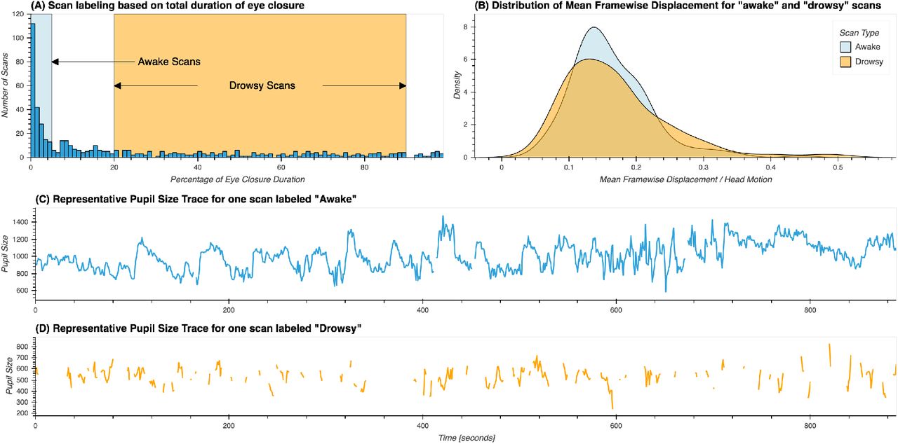
Based on this criteria, 210 scans were labeled as “awake” and 194 were labeled as “drowsy”. The remaining scans were not used in any further analyses. Figure 1.A shows the distribution for percentage of missing eye tracking samples across the original 561 scans, and the ranges we just described for labeling of scans as “awake” and “drowsy”. Figures 1.B & C show representative pupil size traces for each type of scan. Figure 1.D shows the distributions of mean framewise displacement for both types of scans. No significant difference in head motion was found across both scan types using the T-test (T=−1.09, p=0.27) or the Mann-Whitney rank test (H=20412.0, p=0.97).

(A) Distribution of percentage of total eye closure per resting-state scan across the whole sample. Ranges used for the selection of scans marked as “awake” and “drowsy” are depicted by rectangles in light blue and orange respectively. (B) Distribution of mean values of framewise displacement across both groups of scans. (C) Presentative pupil size trace for a scan labeled as “awake”. (D) Representative pupil size trace for a scan labeled as “drowsy”.
Scan Segmentation based on Pupil Size Traces
For all remaining 404 scans labeled as either “awake” or “drowsy” we identified all periods eye opening (EO; i.e., pupil size data available) and eye closure (EC; i.e., pupil size data missing); and recorded their onsets, offsets and durations. This information was used to find periods of continuous EC or EO lasting more than 60 seconds. Such scan segments were used in subsequent analyses as described below.
fMRI Data
Fourth Ventricle Signal Extraction
The HCP structural pre-processing pipeline generates, among other outcomes, subject-specific anatomically based parcellations in MNI space. These parcellations are not restricted to regions within the grey matter (GM) ribbon, but also include subdivisions for white matter (WM) and cerebrospinal fluid (CSF) compartments, one of them being the FV. A group-level FV region of interest (ROI) was generated by selecting voxels that are part of this region in at least 98% of the sample. Figure 2 show this FV ROI overlaid on the mean EPI image across all 404 scans marked as either “drowsy” or “awake”.

Region of interest for the 4th ventricle overlaid on top of the average of the first EPI image from all 404 resting state scans entering the main analyses.
To obtain scan-wise representative FV timeseries, we first removed the initial 10 volumes from the minimally preprocessed data, and then scaled the data by dividing each voxel timeseries by its own mean and multiplying by 100. The representative FV timeseries for each scan was computed as the average across all voxels in this ROI. The representative timeseries for this region was extracted prior to any additional pre-processing to minimize the removal of inflow effects and also minimize partial volume effects.
Frequency Analysis of the 4th Ventricle Signal
First, we estimated the spectral power density (PSD) for each subject’s FV timeseries using python’s scipy implementation of the Welch’s method (window length=60s, window overlap=45s, NFFT=128 samples). We did this both at the scan level (i.e., using complete scan timeseries) and the segment level (i.e., using only segments of continuous EO and EC, as described above). We then compared PSD across scan types (“awake” vs. “drowsy”) and segment types (EC vs. EO). Significant differences were identified using the Kruskal-Wallis H-test at each available frequency step and pBonf<0.05, corrected for the number of different frequencies being compared.
Next, to study the temporal evolution of the FV signal fluctuations centered around 0.05Hz, we also computed spectrograms (i.e., PSD across time) using python’s scipy spectrogram function (window length=60s, window overlap=59s, NFFT=128). We did so for each scan separately, and then computed the average temporal traces of PSD within two different frequency bands:
“Sleep” band: 0.03 – 0.07 Hz.
“Control” band: 0.1 – 0.2 Hz.
The range of the sleep band was selected based on the original work of Fultz et al. (2019) so that it would include the target frequency of interest (0.05Hz). The control band was selected as to exclude respiratory signals as well as the 0.01 – 0.1 Hz band, which contains the majority of neuronally-induced fluctuations in resting-state data (Cordes et al., 2001). In later analyses we refer to the total area under the PSD trace for the sleep band as PSDsleep and for the control band as PSDcontrol.
Figure 3 depicts this process. Figure 3.A shows the average BOLD signal in the 4th ventricle for one resting-state scan from a representative subject. Figure 3.B shows the associated spectrogram, as well as the sleep (green) and control (red) bands. Finally, Figure 3.C shows the average PSD within these two bands of interest (green and red curves). For this particular scan, a strong fluctuation around 0.05Hz appears during the second half of the scan (Figure 3.A). This fluctuation results in an increased PSD for a small range of frequencies around 0.05Hz (Figure 3.B). Such increase becomes clearly apparent when we look at the average PSD traces for the “sleep” and “control” bands in Figure 3.C. While the green trace (“sleep” band) shows large positive deflections during the second half of the scan, that is not the case for the red trace (“control” band).

Evaluation of the temporal evolution of fluctuations around 0.05Hz in the BOLD signal from the 4th ventricle in one representative subject. (A) BOLD timeseries for the 4th ventricle during one representative 15 minutes resting state scan. (B) Spectrogram for the representative time-series depicted in the top panel. Two frequencies bands of interest are marked as colored bands on the sides of the spectrogram: 0.03 – 0.07Hz (sleep band – green shading) and 0.1 – 0.2 Hz (control band – red shading) (C) Average PSD for the two frequency bands of interest: sleep band (green) and control band (red). Bold lines represent the temporal evolution of the average PSD for each band. Shaded area, namely the area under a given PSD trace, represents the total PSD in each band for the whole scan.
fMRI Pre-processing pipelines
Three different pre-processing pipelines were used in this study. The three pipelines take as input minimally pre-processed data available as part of the HCP 1200 data release, which has already undergone steps to account for distortion correction, motion correction and spatial normalization to the MNI template space (Glasser et al., 2013). Here, we now describe the additional steps included in each of our three pre-processing pipelines:
Basic pipeline
minimally pre-processed data followed by: 1) discard initial 10 volumes, 2) spatial smoothing (FWHM = 4mm), 3) intensity normalization dividing by the voxel-wise mean timeseries, 4) regression of motion parameters, their first derivative and slow signal drifts (Legendre polynomials up to the 5th order) and 5) band-pass filtering (0.01 – 0.1 Hz).
CompCor pipeline
similar to the Basic pipeline, except that a set of additional regressors based on the CompCor technique (Behzadi et al., 2007) were included to account for physiological noise in the noise regression step (step 4). Those regressors are the first three principal components of the signal in the lateral ventricles. A subject specific mask for this region was created by eroding by one voxel the homonymous mask created by Freesurfer (Fischl, 2012) and made available as part of HCP 1200 data release.
CompCor+ pipeline
similar to the CompCor pipeline, except that an additional regressor corresponding to the average signal in the FV is also included.
All pre-processing steps, beyond those part of the minimally pre-processing pipeline, were performed with the AFNI software (Cox, 1996).
Correlation analyses: zero-lag
The input for the zero-lag correlation analyses is the output of the “basic” pre-processing pipeline. The voxel-wise maps of correlation between the FV signal (extracted as described in “fourth ventricle signal extraction”) and all voxels in the full brain mask (available as part of the HCP data release) were computed separately for each period of EC and EO longer than 60 seconds. Next, we generated average correlation maps per eye condition by averaging the individual maps for all segments of a given type. For this, we applied a Fisher Z transform prior to averaging. Following averaging, Z-values were converted back to R-values prior to presentation. We then performed a T-test across the population (AFNI program 3dttest+) to identify regions with significant differences in correlation with the FV signal across eye conditions. Finally, histograms of correlation values per eye condition were computed based on the average maps.
Correlation analyses: cross-correlation and lag maps
The RapidTide2 software (https://github.com/bbfrederick/rapidtide ; v1.9.3+40.g951d543) was used to perform cross-correlation analyses. Given, the Rapidtide2 software applies bandpass filtering (also set to 0.01 – 0.1 Hz), inputs to this software were the data from the basic pipeline, excluding the filtering step.
In addition to voxel-wise cross-correlation traces, the Rapidtide2 software also produces a) voxel-wise lag maps, where each voxel is assigned the temporal lag leading to the strongest positive correlation between the source signal (i.e., that from the FV) and the signal in that particular voxel; and b) masks of statistical significance for cross correlation results based on non-parametric simulations with null distributions (n=10,000).
Cross-correlation analyses were conducted at the scan level using only scans labeled as “drowsy”, as those are expected to contain more fluctuations of interest (i.e., those associated with light sleep). To generate group-level lag maps and voxel-wise cross-correlation traces we computed the average across scans taking into account only results rendered significant at p<0.05 at the scan-level. We only show results for voxels where at least half of the scans produced significant cross-correlation results. This averaging approach was followed to avoid non-significant low correlations and noisy lag estimation contributing to the group level results.
Whole-brain connectivity analyses
We were also interested in evaluating the potential effects that unaccounted slow sleep-related fluctuations may have on full brain functional connectivity (FC) matrices. For that purpose, we computed whole-brain FC matrices using the 200 ROI Schaefer Atlas (Schaefer et al., 2017) for the three pre-processing pipelines previously described, namely the “basic” pipeline, the “compcor” pipeline and the “compcor+” pipeline.
For each ROI, a representative timeseries was generated as the average across all voxels part of that ROI. Statistical differences in connectivity between “drowsy” and “awake” scans were then evaluated using Network-based Statistics (Zalesky et al., 2010) using T=3.1 as the threshold at the single connection level, and p<0.05 at the component level (5000 permutations). Finally, results are presented in brain space using the BrainNet Viewer software (Xia et al., 2013).
Global Signal Extraction
The global signal (GS) for each scan was computed as the spatial average of all voxels in the brain mask (distributed with the HCP 1200 data release) using as input the resulting timeseries from the different pre-processing pipelines (as indicated in each result). This brain mask includes voxels from all three tissue compartments, namely grey matter, white matter, and CSF (including the FV). Next, we computed the amplitude of the global signal (GSamplitude) for EC and EO segments as the temporal standard deviation of the global signal within the time periods spanning those segments.
Eye condition prediction
To study how well the presence of fluctuations around 0.05Hz in the FV can help us predict reduced wakefulness, we used a logistic regression classifier that takes as inputs windowed (window length = 60s, window step = 1s) estimates of PSDsleep. A duration of 60s was selected to match the frequency analyses described before. Classification labels were generated as follows. For each sliding window, we calculated the percentage of eye closing time for that window. If that percentage was above 60%, we assigned the label “eyes closed/drowsy”. If the percentage was lower than 40%, we assigned the label “eyes open/awake”. All other segments were discarded given their mix/uncertain nature. The input to the classifier was the average PSDsleep in the corresponding window.
This analysis was conducted using all 404 scans. This procedure resulted in an imbalanced dataset with 311184 samples, of which 233451 (~75%) correspond to “eyes open/awake” class, and the rest (77733; ~25%) to the “eyes closed/drowsy” class. To account for this imbalance, we used a stratified k-fold approach to estimate the generalizable accuracy of the classifier (k=10) and assigned class weights inversely proportional to the frequency of each label during the training. Those analyses were conducted in Python using the scikit-learn library (Abraham et al., 2014).
The same analysis was conducted also using as input the sliding window version of the GSamplitude, a randomized version of the PSDsleep (control case) and using as features both the windowed GSamplitude and the PSDsleep. Significant differences in accuracy across these scenarios was evaluated via T-test (with as many accuracy estimates per classification scenario as k-folds). Additionally, a representative confusion matrix per classification scenario was created by computing median precision values across k-folds.
Results
Eye Tracking
Figure 4 shows the percentage of scans (Y-axis) for which subjects had their eyes closed at a particular fMRI volume acquisition (X-axis). Individual dots represent actual scan counts at each TR, while the black line represents a linear fit to the data. For approximately 10% of scans, subjects had their eyes closed during the first fMRI acquisition. As scanning progresses, the number of scans for which subjects had their eyes closed increases (Linear Fit R=0.96). By the end of the resting state scans, in approximately 40% of scans, subjects had their eyes closed; signaling that as time inside the scanner advances more subjects may have fallen asleep.

Percentage of scans with eyes closed at a given fMRI acquisition. As scanning progresses, the number of subjects with their eyes closed at a given fMRI acquisition (i.e., TR) increases.
Spectral Characteristics of the 4th ventricle signal across scan types
Power Spectral Density (PSD) of the BOLD signal in the 4th Ventricle
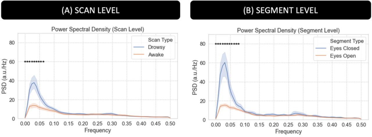
Figure 5.A shows average PSD across all scans labeled as “awake” (orange) and those labeled as “drowsy” (blue). Figure 5.B shows average PSD across all scan segments during which subjects had their eyes closed (EC; blue) for at least 60 seconds and for all scan segments during which subjects had their eyes open (EO; orange) for the same minimum duration. We can observe that PSD is significantly higher for “drowsy” scans as compared to “awake” scans. The same is true for EC segments as compared to EO segments (pBonf<0.05). Significant differences concentrate primarily below 0.06Hz at the scan level, and extents all the way to 0.08Hz when looking at the segment level.

Power Spectral Density (PSD) analysis for the average fMRI signal in the 4th ventricle. (A) Average PSD for “awake” and “drowsy” scans. (B) Average PSD across eyes closed and eyes open segments. In both panels, frequencies for which there is a significant difference (pBonf<0.05) are marked with an asterisk.
Time-frequency analyses for the signal in the 4th Ventricle
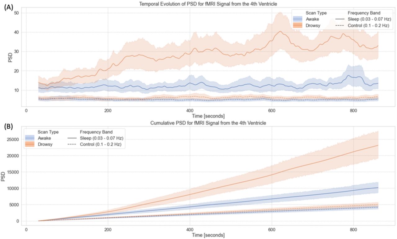
Figure 6 summarizes our results from the time-frequency analyses for the FV signal. First, figure 6.A shows the temporal evolution of the average Power Spectral Density (PSD) in two different bands—namely the sleep band (PSDsleep) and control band (PSDcontrol)—for both “awake” and “drowsy” scans. PSDsleep evolves differently with time for both scan types. For “awake” scans, PSDsleep remains relatively flat for the whole scan duration. Conversely, for “drowsy” scans, the PSDsleep shows an incremental increase as scanning progresses. This increase becomes clearly apparent after the initial 3 minutes of scan. No difference in the temporal evolution of the PSDcontrol was observed across scan types.

Time-frequency analyses for the BOLD signal from the 4th ventricle. (A) Temporal evolution of the power spectral density (PSD) of this signal in two different frequency bands (sleep band: 0.03 – 0.07Hz, control band: 0.1 – 0.2Hz) for scans labeled as “awake” and “drowsy”. (B) Cumulative PSD for the same two bands and scan types shown in the top panel. In both panels, lines show the average across all scans of a given type, and shaded regions indicate 95% confidence intervals. Continuous lines correspond to trends for the sleep band, while dashed lines corresponds to the control band.
As subjects are not expected to close their eyes or fall slept in synchrony, we also looked at cumulative versions of PSDsleep and PSDcontrol as a function of time (Figure 6.B). In this case, we observe a faster increase in cumulative PSDsleep for “drowsy” scans as compared to “awake” scans. This difference becomes clearly apparent approximately after 180 seconds. Conversely, for the cumulative PSDcontrol, we did not observe any difference in the rate of increase across scan types.
Where else in the brain can we observe these sleep-related fluctuations?
Previous work has reported a negative correlation between the sleep-related signal from the FV and the average signal for all cortical grey matter (Fultz et al., 2019). To explore if such a relationship is also present in the current dataset during long periods of eye closure, we conducted two types of correlational analyses: a) zero-lag correlation analysis, and b) cross-correlation analysis with lags between −15s and +15s.
Zero-lag Correlation Analysis
For periods of eye closure (EC, Figure 7.A), we observe wide-spread negative correlations between the sleep-related signal in the FV and grey matter (colder colors). We also observe positive correlation in periventricular regions superior to the FV (warmer colors). Importantly, not all regions correlate with the same intensity. The strongest negative correlations (r < −0.2) concentrate on primary somatosensory regions, primary auditory cortex, inferior occipital visual regions and the occipito-parietal junction. The strongest positive correlations (r > 0.2) appear mostly on the edges of ventricular regions above FV.

(A) Group-level map of voxel-wise average correlation between the signal from the 4th ventricle and the rest of the brain for periods of eye closure longer than 60 seconds. (B) Same as (A) but for periods of eye opening longer than 60 seconds. In both (A) and (B), areas with | R | > 0.2 are highlighted with a black border and no transparency. Areas with |R| < 0.2 are shown with a higher level of transparency. (C) Histogram of voxel-wise average R values across all scan segments for both conditions. A shift towards stronger correlation values can be observed for the eyes closed condition. (D) Significant differences in voxel-wise correlation between eyes closed and eyes open condition (pBonf<0.05).
For eye opening (EO) periods (Figure 7.B), although there is a mostly negative relationship between the signal from the 4th ventricle and the rest of the brain, this relationship is weak (|r|<0.1 everywhere). Figure 7.C shows the distribution of correlation values for both EC (blue) and EO (orange). While for EO correlation values are mostly centered around zero; for EC we can see a bimodal distribution with one peak around −0.2 (corresponding the areas of strong negative correlation within grey matter) and a second positive peak around 0.05 with a long positive tail (corresponding to the strong positive correlations in other ventricular regions). Finally, a test for statistical difference (pBonf<0.05) in voxel-wise correlation values between the EO and EC segments (Figure 7.D) revealed that regions with significant differences mimic those shown in figure 7.A as having the strongest correlations during EC.
Cross-Correlation Analysis
To explore differences in arrival time across the brain, we also conducted voxel-wise cross correlation analyses based on the FV signal using only the “drowsy” scans. Figure 8.A shows the resulting average map of temporal lags, where the color of a voxel represents the lag conductive to the maximum positive cross-correlation value at that location. Lags vary significantly across tissue compartments. Positive lags concentrate in ventricular regions superior to the FV, and negative lags are observed across grey matter. Right-left hemispheric symmetry is present, with longer negative lags appearing on most lateral regions (darker blue) as compared to more medial regions (light blue). Also, although significant correlations can be observed at many locations in the posterior half of the brain, the same is not true for frontal and inferior temporal regions. Next, figure 8.B shows the average cross-correlation trace across all significant voxels. Maximal anticorrelation is observed for a lag of 3s (r=−0.25). Finally, figure 8.C shows cross-correlation traces in six representative voxels. We can observe large variability, with cross-correlation peaks occurring at different times in different locations.

(A) Whole brain lag maps for the signal from the 4th ventricle. Color indicates the temporal lag conductive to maximal positive correlation within the lag range (−15s, 15s). (B) Average cross-correlation trace across all significant voxels. (C) Representative voxel-wise cross-correlation traces for six different locations marked with numbered circles in panel (A).
Contribution to the Global Signal
Figure 9.A shows the distribution of GSamplitude values for the different scan types (i.e., “awake” and “drowsy”). On average, “drowsy” scans have a significantly higher GSamplitude than “awake” scans. Figure 9.B shows that the same is true at the segment level, with significantly higher GSamplitude when computed only using long periods of eye closure, compared to long periods of eye opening. In both cases, GSamplitude has been computed for GS obtained following the “basic” pre-processing pipeline. In addition, table 2.A & B also shows the results of significant tests for GSamplitude, when the GS is obtained following any of the three pipelines described in the methods section. Independently of pre-processing, a significant difference was always observed.

(A) Box plot of GSamplitude across scan types. (B) Box plot of GSamplitude across segment types. (C) Boxplot of PSDsleep across scan types. (D) Boxplot of PSDsleep across scan types.
Significant differences in GSamplitude across scan types (A) and segment types (B) for the different pre-processing pipelines.
Figure 9.C & D show the results for PSDsleep, which was extracted directly from the minimally pre-processed data (see methods). In both, scan-level and segment-level analyses, PSDsleep was significantly higher for states of lowered arousal.
Value as an indirect marker of wakefulness
Scan Ranking in terms of 4th Ventricle PSD and Global Signal
To explore the potential value of the FV fluctuations around 0.05Hz as an indicator of lowered wakefulness, we decided to sort all 404 scans in terms of the total PSDsleep (Figure 10.A). Because the amplitude of the global signal (GSAmp) has been previously stablished as a good indicator of wakefulness, we also sorted scans according to this second index (Figure 10.B). In figures 10.A & B, each scan is represented as a vertical bar whose height is either the PSDsleep (10.A) or GSAmp (10.B). Each bar is colored according to whether that particular scan was labeled as “awake” (orange) or “drowsy” (light blue). In both plots, there is a higher concentration of “drowsy” scans on the left (i.e., higher PSDsleep or GSAmp). Conversely, there is a higher concentration of “awake” scans on the other end of the rank. This profile, of more “awake” than “drowsy” scans among those with higher PSDsleep or GSAmp, and the opposite as we go down on the rank becomes more apparent when we look at the relative proportions of each scan type in intervals of 100 scans (Figures 10.C & D). Within the top 100 ranked scans, the number of “drowsy” scans is more than double the number of “awake” scans. Conversely, we look at the bottom 104 ranked scans, these proportions have reversed. Finally, it is worth noticing that PSDsleep and GSAmp based rankings, although similar at the aggregate levels described here, are not equal on a scan-by-scan basis. In other words, the specific rank of a given scan is not necessarily the same for both ranking schemes.

(A) Ranked scans according to the total PSD in the sleep band (0.03Hz – 0.07Hz) for the signal from the 4th ventricle. (B) Ranked scans according to the amplitude of the global signal. In both (A) and (B), each scan is represented by a vertical bar. The color of the bar indicates whether a given scan was labeled “drowsy” or “awake” based on the total amount of time subjects kept their eyes closed during that particular scan. (C) Proportion of “drowsy” and “awake” scans in rank intervals (1 – 100, 101 – 200, 201 – 300, 301 – 304) for PSD-based ranks. (D) Proportion of “drowsy” and “awake” scans in rank intervals (1 – 100, 101 – 200, 201 – 300, 301 – 304) for GS-based ranks.
Classification accuracy at the segment-level
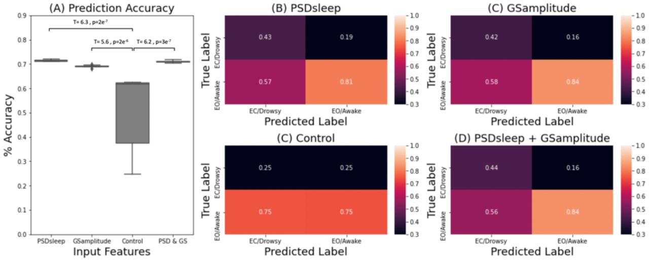
We also evaluated the ability of PSDsleep to predict wakefulness at the segment level (i.e., 60 seconds segments), and how it compares to that of GSamplitude. Figure 11 shows results for this last set of analyses. Figure 11.A shows prediction accuracy results for four different classification scenarios: a) when PSDsleep is the only input feature, b) when GSamplitude is the only input feature, when both PSDsleep and GSamplitude are used as input features (PSD+GS) and d) when PSDsleep is the only feature and labels are randomized (control condition). Accuracy was significantly higher for the three non-control scenarios (i.e., PSDsleep, GSamplitude, PSD+GS) when compared to the control condition. Although significant differences were also observed among the three non-control scenarios (not marked in figure 11.A), in this case, differences in accuracy in absolute terms was very small (<0.02). Confusion matrices (Figures 11.B – E) confirm that although there are clear differences in precision values between the control and the other three scenarios, that is not the case among the three non-control cases.

(A) Prediction accuracy for a logistic regression classifier with different set of input features: PSDsleep, GSamplitude, randomized PSDsleep (control) and PSDsleep + GSamplitude. (B-D) Confusion matrices for each case. Numbers indicate precision for the different classes.
Effects on whole-brain functional connectivity matrices
Figure 12 shows the results for the whole-brain functional connectivity analysis. Both average connectivity matrices per scan type (e.g., “awake” or “drowsy”) and significant differences in connectivity between both types of scans were computed for three different pre-processing scenarios (i.e., Basic, Compcor, and Compcor+) to evaluate the effect that fluctuations in the frequency range 0.03 – 0.07Hz observed in the FV may have on estimates of functional connectivity across the brain. Figure 12.A-E show results for the basic pipeline where no signals from ventricular compartments are regressed. Figure 12.F-J show results when CompCor regressors (signals from the lateral ventricles) are included as additional regressors. Finally, Figure 12.K-O show results when the average signal from the FV is also included as an additional regressor.
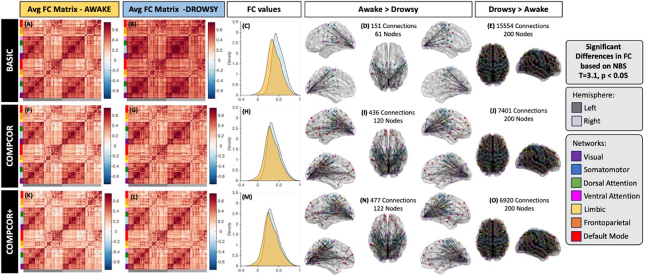
Whole-brain functional connectivity results. (A-E) Results for the basic pre-processing pipeline. (F-J) Result for the CompCor pipeline. (K-O) Results for the CompCor+ pipeline. In all rows the left most column shows the average connectivity matrix for all “awake” scans. The next column shows the average connectivity matrix for all “drowsy” scans. The middle column shows the distribution of correlation values across the whole brain for both scan types: drowsy in blue; and awake in orange. Finally, the last two columns show connections that were significantly different between the two scan types. The left most of these two columns show connections with stronger correlation for “awake” scans relative to “drowsy”. Conversely, the right most column shows those that are stronger for “drowsy” relative to “awake” scans. Significance was evaluated using Network-based statistics (T> 3.1, 5000 permutations, p<0.05 at the component level).
While average connectivity matrices for all three scenarios look quite similar for the “awake” scans (Figure 12.A, F & K); for “drowsy” scans we can observe stronger overall connectivity across most regions for the basic pipeline (Figure 12.B) compared to the two other pipelines that include as regressors signals from ventricular compartments (Figure 12.G & L). Additionally, no large differences in overall levels of connectivity values are observed between Figure 12.G (CompCor) and Figure 12.L (CompCor+) suggesting that regression of signals from ventricular regions superior to the FV (as it is done in CompCor) suffice to remove the sleep related fluctuations that constitute the target of this work.
The same trends are clearly observed in terms of the distribution of connectivity values across the whole brain presented in Figure 12.C, H & M. While for basic pre-processing (Figure 12.C) the distribution of connectivity values for “drowsy” scans is clearly shifted toward positive values relative to the distribution for “awake” scans. Such shift is not apparent in the other two pre-processing scenarios (Figure 12.H & M).
When looking at significant differences in connectivity between “awake” and “drowsy” scans, we can again observe that not taking into consideration the slow fluctuations from the FV (or their correlated counterparts in superior ventricular regions) leads to a decrease in our ability to detect connections that are stronger during “awake” scans compared to “drowsy” scans (Figure 12.D,I & N) as well as to an overestimation of the number of connections with significantly stronger connectivity in the other direction (“drowsy” greater than “awake”; Figure 12. E, J & O). It is worth noticing that for the “awake” > “drowsy” comparison, significand differences in functional connectivity among frontal regions of the default mode network, and posterior parts of the brain only become apparent when ventricular signals are regressed during pre-processing.
Discussion
Previous work has shown that strong fluctuations (at approx. 0.05 Hz) appear in the FV when subjects descend into sleep, and that strong anticorrelated fluctuations of equal frequency can be observed in grey matter with an optimal delay of 2s (Fultz et al., 2019). Here, we extend those observations in several ways. First, we demonstrate that equivalent ventricular sleep-related fluctuations can be observed in data that was not necessarily optimized for capturing inflow effects. Second, we demonstrate that although overall optimal lag across GM does indeed peak at 2 seconds, there is substantial variability in terms of optimal lag and cross-correlation profiles across the brain (Figure 8). Third, we show that the presence/absence of this sleep-related signal can, to some extent, help rank scans according to arousal levels, when better concurrent measures of arousal (e.g., those derived from concurrent EEG or eye tracking recordings) are not available. Forth, we show that these sleep-related fluctuations only minimally explain the ability of the global signal to track fluctuations in arousal, as regression of these fluctuations does not eliminate significant differences in GSamplitude across scan types. Fifth, we demonstrate that not accounting for the potential presence of these signals during pre-processing can significantly affect estimates of functional connectivity. Finally, this work also constitutes an important reproducibility study regarding the presence of those ultra-slow fluctuations in fMRI data during sleep with a much larger sample than those used in the past (i.e., (Fultz et al., 2019): 13 participants, (Song et al., 2019): 58 participants, here: 561 scans from 174 participants).
Spatiotemporal profile
Fluctuations around 0.05Hz, anticorrelated with their counterpart in the FV, appear in several grey matter regions in “drowsy” scans. In particular, the strongest anticorrelations occur in visual, MT, sensorimotor, and supplementary motor cortex (Figure 7). This pattern overlaps with that previously reported by Song et al. (2019) for fluctuations of similar frequency profile that appear in fMRI recordings during light sleep and track EEG spindles (a key signature of light sleep; (Gennaro and Ferrara, 2003)). Additionally, Song et al. (2019) also reported that these oscillations first appear in thalamic and sensory regions; and from there, they propagate to prefrontal regions and the cerebellum. Here, cross-correlations results for the FV signal (Figure 8.A), show a similar pattern with sensory regions having earlier lags than frontal and cerebellar regions. These converging observations emerge from a very different set of methods and assumptions. In the case of Song et al., the authors relied on concurrent EEG measures to detect periods of light sleep and subsequently evaluate changes in frequency profiles at the regional level relative to wakefulness. Here, we simply studied patterns of correlation with the FV signal on scans marked as “drowsy” based on eye tracking recordings. The agreement across both studies with respect to the spatiotemporal profiles for these ultra-slow fluctuations suggest that the bulk of our observations are indeed related to periods of light sleep, and not simply to subject’s lack of compliance regarding instructions to keep their eyes open. This is important, as with ET alone it is not possible to separate these two potential scenarios, and as we shall discuss below, the presence of 0.05Hz in ventricular compartments may provide insight about sleep incidence on a given resting-state sample when no additional recordings are available.
Relationship to inflow
Fultz et al. (2019), who originally observed the FV fluctuations targeted in this work, did so on data acquired with a protocol optimized for detecting inflow effects in this region (i.e., TR=367ms; FV intersecting the lower boundary imaging edge). This protocol selection was motivated by the hypothesis that CSF flow reverses during sleep (Grubb and Lauritzen, 2019), and that such reversal would lead to strong inflow effects in this ventricular region. Here, we use the HCP 7T resting-state data sample, which is less influenced by inflow effects in the FV with a TR approximately three times longer (TR=1s), and with the FV not sitting near the lower boundary of the imaging field of view (FOV; see Suppl. Figure 2). Nevertheless, despite those differences in acquisition, we could still find strong fluctuations around 0.05Hz in the FV for “drowsy” scans (e.g., those with long periods of eye closure) relative to “awake” scans (Figure 5.A); and for EC segments longer than 60 seconds, relative to equivalently long segments of EO (Figure 5.C). These observations suggest that sleep-related physiological fluctuations in the FV can be found in “typical” fMRI datasets, even if those were not necessarily optimized to capture inflow effects.
While we replicate the observed MRI signal fluctuations from Fulz et al, our data and analyses do not elucidate the precise physiologic and biophysical mechanisms behind these signals. HCP data used here was acquired at a higher field (7T vs. 3T), and with a slightly larger flip angle (45 vs. 32-37) than that of Fulz et al. Inflow effects tend to be more prominent at higher fields and at larger flip angles (Gao and Liu, 2012). Second, in the HCP data, the FV sits, on average, somewhere between slice 19 and slice 27. Given the use of a multi-band sequence (Feinberg and Setsompop, 2013) with factor (MB=5) and a number of slices equal to 85 in the 7T HCP protocol, the minimal critical imaging velocity for some slices sitting over the FV is 54.40mm/s. Awake CSF maximal velocity ranges between 20-80mm/s in healthy adults (Korbecki et al., 2019; Lee et al., 2004; Nitz et al., 1992). Although the velocity for reversed CSF flow during sleep might be different, Fultz et al. already reported fast events observable four slices away from the lower boundary of the FOV, which would require, for their protocol, CSF velocities above 68mm/s. These numbers suggest that inflow effects may be still observable in the HCP data, even if the location of the slices and the TR is not optimally sensitized. The same might be true for other data acquired with multi-band protocols, and additional research should elucidate how often these, potentially undesirable, fluctuation are present in resting-state datasets. This is important, given one can expect a third of subjects to fall asleep within 3 minutes of scan onset (Tagliazucchi and Laufs, 2014), and that— as we shall discuss below—these fluctuations can significantly affect estimates of functional connectivity.
Another possibility is that fluctuations with a similar frequency profile may emerge in ventricular regions during sleep due to non-inflow-related phenomena. Future research could rely on concurrent multi-echo fMRI and EEG to answer this question. While EEG can provide accurate information about sleep staging, multi-echo fMRI—which refers to the concurrent acquisition of fMRI at multiple echo-times (Posse et al., 1999)—can separate signal fluctuations of BOLD (not inflow-related) and non-BOLD (inflow-related) origin based on how their amplitudes are modulated by the different echo times (Caballero-Gaudes et al., 2019; Gonzalez-Castillo et al., 2016; Kundu et al., 2011). Alternative ways to test the inflow nature of this phenomena would be to acquire fMRI data at multiple flip angles or repetition times (TR). These two imaging parameters affect the amount of T1-weigthing present on the recorded signals, and as such would have a strong modulatory effect on inflow-related fluctuations (Gao and Gore, 1994; Gao and Liu, 2012). Similarly, one could also acquire data using two different slice geometries: one with slices parallel to the hypothesized direction of flow (e.g., sagittal slices), and one perpendicular to it (e.g., axial slices). Inflow-related fluctuations for the hypothesized direction of flow should only be present in the perpendicular acquisition (Gao and Liu, 2012). Finally, researchers could also use outer volume saturation techniques to attempt nulling fluctuations due to incoming fluid from anatomical regions right underneath the imaging field of view.
Effects on functional connectivity
Strong zero-lag correlations between slow fluctuations in the FV and other brain regions were observed in subjects that kept their eyes closed for long periods of time (and possibly fell asleep). Positive zero-lag correlations occurred for other ventricular regions such as the third and lateral ventricles (Figure 7.A). Negative zero-lag correlations were observed in many grey matter regions, including primary cortexes, and insular regions. Additionally, cross-correlation analyses revealed that optimal lags (i.e., those leading to maximal positive correlation) are also heterogenous across the brain (Figure 8). Given the spatial heterogeneity—in terms of strength and lags—of these fluctuations, they have the potential to act as confounding effects when estimating functional connectivity, in a similar way to how systemic fluctuations in brain physiology can elicit structured patterns of functional connectivity that are not neuronally driven (Chen et al., 2020; Tong et al., 2015). In fact, when pre-processing does not account for these sleep-related fluctuations, wide-spread significant differences in connectivity between “awake” and “drowsy” subjects can be observed (Figure 12). Today, in most resting-state studies, such differences would be ignored, and all resting-state scans would likely be considered equivalent. This can translate into the undesired mixture of two distinct connectivity profiles into one that may not be easily interpretable, as it does not represent the average of a homogenous sample (see (Liu and Falahpour, 2020) for a discussion of a similar concern specific to vigilance).
Importantly, when the top three principal components describing the signals in the lateral ventricles are included as nuisance regressors in the analyses—a pre-processing practice commonly known as the CompCor method (Behzadi et al., 2007)—, the distribution of connectivity estimates across the whole brain becomes more similar for “drowsy” and “awake” scans (Figure 12.H). In addition, the sensitivity and specificity for detecting differences in functional connectivity between “awake” and “drowsy” subjects increase (Figure 12.D, E, I and J). For example, the percentage of connections with significantly stronger connectivity for “drowsy” compared to “awake” scans decreases from 78% (15554 connections) to 37% (7401 connections). Conversely, the percentage of connections that are significantly weaker for “drowsy” compared to “awake” subjects increases from 0.75% (151 connections involving 60 ROIs) to 2.2% (436 connections involving 120 nodes).
These gains in sensitivity and specificity lead to better agreement with previous findings regarding connectivity changes during eye closure and sleep. When ventricular signals are not included as nuisance regressors during pre-processing, comparison of connectivity patterns for “drowsy” and “awake” scans produced two main observations: a) the number of connections with increased connectivity during “drowsy” scans is much larger than those that show a decrease in connectivity; and b) most decreases in connectivity for “drowsy” scans involve visual regions. These observations persist if ventricular signals (including the sleep-related signal target of this work) are removed during pre-processing. Moreover, removal of those nuisance signals leads to the additional observation of decreased intra-network connectivity for “drowsy” scans in the visual, attention and default mode networks, as well as between nodes of the visual network and frontal eye field regions from the dorsal attention network. All these observations agree with those recently reported by Agcaoglu et al. (2019) when comparing eyes open to eyes closed resting-state scans. One key discrepancy between our results that those of Agcaoglu et al., is that we also observed decreased connectivity between motor and visual regions in “drowsy” scans. Yet, such trend has also been previously reported by Van Dijk and colleagues (2010) when comparing eyes open vs. eyes closed; suggesting this pattern is not unique to this dataset. Among the changes only observable when ventricular signals are removed, we encounter a decrease in connectivity between anterior and posterior nodes of the default mode network, which is a key signature of sleep (Horovitz et al., 2009). Similarly, we also observed decreased connectivity for regions of the dorsal and ventral attention network. Reduced connectivity in fronto-parietal networks during sleep is another common finding in the literature (Larson-Prior et al., 2009; Picchioni et al., 2013) that is consistent with a behavior, sleep, that is characterized by reduced attention towards the external environment. Overall, these results suggest that removal of sleep-related ultra-slow fluctuations observable in ventricular regions is key to properly identifying neuronally-induced changes in functional connectivity that accompany eye closure and sleep.
Finally, the gain in sensitivity and specificity for the CompCor+ relative to the CompCor pipeline suggests that, when available, it may be beneficial to include an additional regressor for the FV during pre-processing. As Suppl. Fig. 2 shows, it is possible for the original CompCor method to capture residual inflow effects in superior ventricular regions because, for the particular acquisition parameters of the HCP sample (85 slices, MB=5), first shot slices (marked in red) cut through these superior ventricular regions. Yet, that may not necessarily be the case for other protocols. As such, it is advisable to include an additional FV regressor whenever possible (i.e., if the FV is part of the imaging FOV). For example, in our data, despite superior regions having traces of residual inflow effects, adding an additional regressor for the FV helped with sensitivity and specificity of connectivity changes. We attribute this marginal increase in the CompCor+ pipeline, relative to CompCor, to the fact that the targeted sleep-related fluctuations have different lags across the brain; and having an additional regressor with a different lag—relative to that in superior ventricular regions—might have help better isolate and remove this nuisance component.
Relationship to the global signal
It is well established that the standard deviation of the global signal (GSamplitude) increases when vigilance decreases (Wong et al., 2013) and when subjects fall asleep (Fukunaga et al., 2006; Horovitz et al., 2008; Larson-Prior et al., 2009). In agreement with these prior findings, here we observed a significantly higher GSamplitude for “drowsy” scans compared to “awake” (Figure 9.A). Similarly, we also found a significantly higher GSamplitude for long periods of eye closure compared to long periods of eye opening (Figure 9.B). Importantly, these differences remain significant for all other pre-processing pipelines, including those that attempt to remove FV related fluctuations (Table 2.A & B). This suggests that the ultra-slow sleep-related fluctuations being studied here are not the primary driver of differences in GSamplitude across wakefulness states. This may be initially counterintuitive given those sleep-related fluctuations are quite strong and widely distributed in space. Yet, for any spatially distributed signal to be a key contributor to the GS, such signal ought to appear in synchrony across the brain. Otherwise, positive and negative contributions from different locations may cancel each other (see (Liu et al., 2017) for a detailed description of the GS as a measure of synchronicity across the brain). Our results suggest that the reported heterogeneity regarding temporal lags (Figure 8) suffice to produce an overall effect that it is not a key component responsible for the increase in GSamplitude that accompanies decreases in wakefulness. This is not to say that such fluctuations have no effect at all. As tables 2.A & B show, the T-statistic for significant differences in GSamplitude between “awake” and “drowsy” scans (and for eyes open vs. eyes closed segments) does decrease for pre-processing pipelines that try to account for signals that correlate with those present in the ventricles (including the FV), yet not to a point of eliminating significance. Ultimately, what this suggests, is that differences in GSamplitude cannot be attributed solely to physiological effects that create an imprint in ventricular regions (e.g., cardiac, respiration, sleep-related inflow), and that other effects constrained to grey matter (and therefore more likely to be neuronal) are more important.
Ability to predict sleep
It has been previously shown that approximately a third of subjects from the 3T resting-state HCP sample fell asleep within three minutes from scan onset (Tagliazucchi and Laufs, 2014). Here we report on a similar pattern for the 7T HCP sample (Figure 6). While that earlier report on the 3T sample relied on a hierarchical tree of pre-trained support linear vector machines, here we base our observation on the progressive increase in PSDsleep for the FV signal. For the initial 180 seconds of scanning, average PSDsleep traces for “awake” and “drowsy” scans overlap. Beyond that temporal landmark, PSDsleep for “drowsy” scans rises above that of “awake” scans. Conversely, the PSD for the control band (which excludes the 0.05Hz signals of interest) did not differ across scan types irrespective of time; demonstrating the specificity of the effect to the “sleep” band. It is worth noticing that these patterns are clearly observed despite the large confidence intervals associated with across-scans averaged PSDs (Figure 6.A); which emanate from the fact that subjects fall asleep at different moments. Yet, because we can expect a monotonic increase in the number of subjects that fall asleep as scanning time increases, a clearer pattern emerges when looking at cumulative PSDs (Figure 6.B). While the cumulative PSDcontrol for “drowsy” and “awake” scans have equivalent small increases with time; PSDsleep traces clearly diverge across scan types, with “drowsy” scans showing a much faster increase, particularly after approx. 200 seconds from scan onset. These results demonstrate that an easily implementable metric, such as the PSDsleep of the FV, can provide equivalent information about the progressive descent into sleep of a resting-state sample to that obtained using relatively more complex machine learning procedures.
Similarly, sorting scans based on average PSDsleep produced a list of scans (Figure 10.B) with “drowsy” scans appearing in higher proportion (67 drowsy / 33 awake) at the top of the rank (e.g., higher average PSDsleep levels), and “awake” scans appearing at higher proportion (74 awake / 30 drowsy) at the bottom of the rank (e.g., lower average PSDsleep levels). Unfortunately, the rank is not perfect, meaning there is no certainty that a particular scan near one end of the ranking (e.g., scan ranked 400/404) is of one specific type (e.g., “awake”). Several reasons contribute to this situation. First, the dichotomic labeling system (“drowsy” / “awake”) based on the presence/absence of long periods of eye closure may be too simplistic to represent the heterogeneity of sleep patterns present in the data. Similarly, a single number (average PSDsleep) may not suffice to characterize the wakefulness profile of complete scans with alternating periods of wakefulness and sleep of different durations and intensity. Second, while the absence of long periods of eye closure can be confidently associated with wakefulness, the presence of long periods of eye closure does not necessarily mean sleep. As such, some scans labelled here as “drowsy”, may not include sleep periods, and simply capture the fact that subjects stopped complying with the experimental request to keep their eyes open. Finally, another contributing factor might be that not every instance of increase PSDsleep is necessarily associated with a period of light sleep. A closer look at some of the ranking “misplacements” at the top of the rank—namely “awake” scans with high average PSDsleep (Suppl. Fig. 3) shows that in some instances (subjects A and B) periods of elevated PSDsleep coincide with peaks of head motion (black arrows); yet that is not always the case (blue arrows). Although we did not find a significant difference in head motion across scan types, examples such as these suggest that strong ultra-slow fluctuations in the FV can indeed sometimes appear due to motion, decreasing the accuracy of PSDsleep as a frame-to-frame marker of sleep at the individual level. Importantly, it is also possible to observe periods of elevated PSDsleep that do not overlap with periods of higher motion or eye closure (e.g., subjects C & D in Supp. Fig. 3). This suggests that fluctuations at around 0.05Hz in the FV are not exclusive to light sleep and can also occur during wakefulness in the absence of motion. One plausible explanation for these occurrences is variation in cardiac and respiratory function. Because concurrent respiratory and cardiac traces are not available for these data, we could not confirm this hypothesis.
Finally, we also evaluated the ability of PSDsleep to predict wakefulness (e.g., eyes open/awake vs. eyes closed/drowsy) at a temporal resolution of 60 second segments; and compared its ability to that of GSamplitude. Both metrics can significantly predict those labels with accuracies significantly higher than what happens if labels are randomized (Figure 11). The value of GSamplitude as a marker of vigilance/arousal is well stablished. Our result suggests that the spectral content around 0.05Hz of the FV signal (i.e., PSDsleep) can be equally informative, despite this signal being extracted from a non grey-matter region. This highlights the importance of modeling the many physiological changes that accompany descent into sleep (Duyn et al., 2020; Özbay et al., 2019), and their effects on fMRI recordings and its derivatives (e.g., functional connectivity) If the classifier is given both metrics as input features, accuracy levels barely changed suggesting the information provided by these two metrics was quite similar. As originally stated, our goal was to keep methods as simple as possible, and that was the reason why we chose a simple logistic regressor for this set of analyses. It is possible that more advanced classification algorithms (e.g., support vector machines, neuronal networks) might be able to find complementary bits of information in both traces, and therefore the fact that the accuracy for a logistic regression machine barely improved when both metrics are combined should not be taken as evidence that the same will occur with other models.
In summary, PSDsleep can be a valuable marker of decreased arousal at both the scan and segment level, yet its accuracy when combined with simple raking/classification methods is insufficient to unequivocally derive the state of a subject during a given scan or portion of it. That is not to say, that in absence of additional concurrent measures, PSDsleep has no value. Our results demonstrate otherwise. For example, it can be used to check basic properties of a given sample such as the overall propensity of subjects to fall asleep as a function of time. It can also separate scan segments into two categories (i.e., eyes open/awake, eyes closed/drowsy) with up to 70% accuracy. Yet, it is worth noticing that we did not find any substantial benefits by relying on PSDsleep, as opposed to GSamplitude for this purpose. As such, whether to rely on one or the other metric is not clear at this point. For datasets with limited imaging field of view that do not include the FV the choice is clear. When the FV is available, PSDsleep represents an alternative to GSamplitude that is free of direct neuronal contributions (as it is based on the signal from a ventricular compartment), which may help better interpret results in some instances.
Conclusions
Resting-state data is a chief component of today’s non-invasive human neuroimaging research (Essen et al., 2013; Miller et al., 2016). Despite its long history (Biswal, 2012; Snyder and Raichle, 2012), there are many open questions regarding what mechanisms lead to the formation of resting-state networks and their time-varying profiles (Gonzalez-Castillo et al., 2021). One such question is the role that shifts in vigilance and arousal play in shaping resting-state results (Laumann et al., 2016; Tagliazucchi and Laufs, 2014), which is rarely explored because it requires concurrent electrophysiological or eye tracking recordings. Here we explored how CSF flow reversal during light sleep (Fultz et al., 2019) can be exploited to extract information about arousal patterns. Our results demonstrate that it is possible to detect this phenomenon in data with relatively small inflow weighting, its value as a marker of arousal in absence of a better metric, its relationship to the global signal, its nuisance effects on functional connectivity estimates, and how to minimize those. Overall, this work adds to an important body of literature stressing the confounding effects on unmodeled physiological phenomena with spatial structure that resembles that of commonly observed resting-state networks (Birn, 2012; Chen et al., 2020; Tong et al., 2015).
This work is based on the 7T HCP resting-state sample, which is the basis of many neuroimaging studies today. Our results show that this sample, as it is the case with the 3T sample (Tagliazucchi and Laufs, 2014), contain substantial fluctuations in wakefulness both within- and across-subjects, and that their effects should be considered when interpreting results.
Supplementary Figures

Representative cases of final corrections to eye pupil timeseries once those have been interpolated to a sampling rate of 1Hz. (A) In some cases, following interpolation, we observed the presence of isolated samples scattered during long periods of eye closure (red dots). If those samples are not removed, these long periods of eye closure would not be identified as such. To avoid that, we removed any isolated sample with missing data on both ends. (B) Similarly, we observed individual gaps of a single sample breaking long periods of eye closure (red arrow). In those instances, those missing samples were interpolated (red trace).

Acquisition slices imposed on the first EPI volume of two representative subjects. All acquisition slices are marked as green horizontal lines, except those associated with the first shot, which are marked in red. There are five red horizonal lines as the multi-band factor of this data was set to five. In both subjects we can see that at least one such red line traverses the lateral ventricles.

The top panel shows a zoom-in version of the scan rank based on PSDsleep (Figure 9.A). The first four “miss-ranked” subjects are marked as A, B, C and D. Those are “awake” scans that show a high level of PSDsleep. Below this first panel, we show traces of PSDsleep (green) and framewise displacement (grey) for the four subjects. Additionally, we mark periods of eye closure with red blocks. Black arrows indicate instances where increases in PSDsleep are accompanied by spikes in head motion. Blue arrows show instances of head motion that are not accompanied by an increase in PSDsleep. Finally, subjects C & D are good examples of subjects that show periods of elevated PSDsleep in absence of eye closure or motion spikes.
Acknowledgements
This research was possible thanks to the support of the National Institute of Mental Health Intramural Research Program (ZIAMH002783). Portions of this study used the high-performance computational capabilities of the Biowulf Linux cluster at the National Institutes of Health, Bethesda, MD (biowulf.nih.gov).


