

ABSTRACT
The hippocampus consists of a stereotyped neuronal circuit repeated along the septal-temporal axis. This transverse circuit contains distinct subfields with stereotyped connectivity that support crucial cognitive processes, including episodic and spatial memory. However, comprehensive measurements across the transverse hippocampal circuit in vivo are intractable with existing techniques. Here, we developed an approach for two-photon imaging of the transverse hippocampal plane in awake mice via implanted glass microperiscopes, allowing optical access to the major hippocampal subfields and to the dendritic arbor of pyramidal neurons. Using this approach, we tracked dendritic morphological dynamics on CA1 apical dendrites and characterized spine turnover. We then used calcium imaging to quantify the prevalence of place and speed cells across subfields. Finally, we measured the anatomical distribution of spatial information, finding a non-uniform distribution of spatial selectivity along the DG-to-CA1 axis. This approach extends the existing toolbox for structural and functional measurements of hippocampal circuitry.
INTRODUCTION
The hippocampus is critical for episodic and spatial memories1–3, but the neural computations underlying these functions are not well understood. The trisynaptic circuit linking entorhinal cortex (EC) to dentate gyrus (DG), DG to CA3, and CA3 to CA1 is believed to endow the hippocampus with its functional capabilities. Since the circuit was first described in the anatomical studies of Ramon y Cajal over a century ago4, considerable work has focused on each of the major hippocampal subfields (CA1-3 and DG) to identify their roles in hippocampal processing. The resulting body of literature has indicated that the subfields have related, but distinct roles in pattern separation and completion5–14, response to novelty15–19, and the encoding of social variables20–22. Additionally, there appear to be differences between the subfields in place field stability19,23,24. Although this work has increased our understanding of each of the subfields individually, it is not clear how neuronal activity is coordinated across the hippocampus.
This lack of knowledge comes, in part, from the technological limitations that prevent the recording of neuronal populations across hippocampal subfields in the same animal. Historically, electrophysiology has been the principal tool used to study the hippocampus. Electrophysiological recordings have the advantage of high temporal resolution and can directly measure spiking, but they are typically limited to small numbers of neurons in particular subfields. Additionally, localization of recorded neurons within the hippocampus is approximate, requiring post-hoc histological analysis to estimate the position of the electrode tracks, and the distances between the recorded neurons and the electrode sites are poorly defined. In recent years, calcium imaging approaches (i.e. single photon mini-endoscopes and two-photon microscopy) have been used to record hippocampal activity, allowing for the simultaneous measurement of large numbers of neurons with known spatial relationships24–29. However, these approaches require aspiration of the overlying neocortex and are generally restricted to a single subfield for each animal.
Taken together, current experimental techniques are limited in their ability to: (1) record response dynamics and coordination across the hippocampus, (2) identify and distinguish between different neural subtypes, (3) allow for the chronic recording of cells across subfields, and (4) resolve key cellular structures, such as apical dendritic spines.
To address these challenges, we have developed a procedure for transverse imaging of the trisynaptic hippocampal circuit using chronically implanted glass microperiscopes. As has been found with previous studies using implanted microprisms in cortex30–33, the neural tissue remained intact and healthy for prolonged periods of time (up to 10 months), and both dendritic structure and calcium activity could be repeatedly measured in behaving mice. Optical modeling and point spread function measurements showed that axial resolution is decreased compared to traditional cranial windows, but is sufficient to image individual apical dendritic spines in hippocampal neurons several millimeters below the pial surface. Using this approach, we quantified spine turnover in CA1 apical dendrites across days. We then measured functional responses from CA1, CA3, and DG in head-fixed mice as they explored a floating carbon fiber arena34,35. We found neurons in all regions whose activity met criteria to be considered place cells (PC) and speed cells (SC). Further, we found non-uniform distributions of spatial information across the extent of the DG-to-CA1 axis, in agreement with earlier electrophysiological studies36–38. Taken together, this approach adds to the existing neurophysiological toolkit by enabling chronic structural and functional measurements across the entire transverse hippocampal circuit.
RESULTS
Optical access to the transverse hippocampus using implanted microperiscopes
In order to image the transverse hippocampal circuit using two-photon (2P) imaging, we developed a surgical procedure for chronically implanting a glass microperiscope into the septal (dorsomedial) end of the mouse hippocampus (Fig. 1A; see Methods). For imaging CA1 only, we used a 1 mm × 1 mm × 2 mm microperiscope (v1CA1; Fig 1B, left), and for imaging the entire transverse hippocampus (CA1-CA3, DG), we used a 1.5 mm × 1.5 mm × 2.5 mm microperiscope (v2HPC; Fig 1B, right). The microperiscope hypotenuse was coated with enhanced aluminum in order to reflect the imaging plane orthogonally onto the transverse plane of the hippocampus (Fig. 1C, D). To insert the microperiscope, we made a single incision through the dura and tissue, then lowered the tip of the microperiscope into the incision, pushing the cortical tissue medially. Although this approach eliminated the need for the aspiration of cortical tissue typically performed prior to hippocampal imaging25, it nonetheless results in severed connections and compressed tissue medial to the implant. Since the septal end of the hippocampus is affected by the implant, we used immunohistochemistry to quantify the effect of microperiscope implantation on microglia and astrocyte proliferation as a function of distance from the prism face (Fig. 1E). Similar to previous research using microprism implants31, we found an increase in the prevalence of astrocytes and microglia <200 μm from the microperiscope face, but the prevalence decreased past this distance and was indistinguishable from the control hemisphere 300-400 μm from the microperiscope face (Fig. 1F).

(A) Three-dimensional schematic87 illustrating microperiscope implantation and light path for hippocampal imaging.
(B) Schematics88 showing the imaging plane location of v1CA1 (1 mm imaging plane, 2 mm total length) and v2HPC (1.5 mm imaging plane, 2.5 mm total length) microperiscopes.
(C) Tiled average projection of the transverse imaging plane using the v2HPC microperiscope implant in a Thy1-GFP-M transgenic mouse. Scale bar = 100 μm.
(D) Enlarged images of hippocampal subfields (CA1, CA3, DG) corresponding to the rectangles in (C). Scale bar = 50 μm.
(E) Example histological section stained for microglia (S100 - red) and astrocytes (GFAP - green). Scale bar = 300 μm.
(F) Quantification of microglia and astrocyte density as a function of distance from the prism face, normalized to the density in the unimplanted contralateral hemisphere (n = 2 mice; mean ± bootstrapped s.e.m.).
Use of the microperiscope requires imaging through several millimeters of glass, which could cause beam clipping or optical aberrations, resulting in decreased optical resolution. To determine the extent to which this occurred in our experiments, we modeled the expected point spread function and compared it to the experimentally-determined point spread function measurements using fluorescent microspheres (Fig. S1). Compared to a standard cranial window, we found that the lateral resolution of the microperiscope, measured as the full width at half maximum (FWHM) of the fluorescent microsphere profile, was similar to a standard cover slip (coverslip: 0.7 μm; v1CA1 microperiscope: 1.0 μm; 2.5 mm microperiscope: 0.7; Fig. S1), while the axial resolution of the craniotomy window with the microperiscope was significantly lower (coverslip: 3.0 μm; 2 mm microperiscope: 9.0 μm; 2.5 mm microperiscope: 7.0 μm; Fig. S1). Optical modeling indicates that the decrease in axial resolution is predominantly due to clipping of the excitation beam, resulting in a reduction of the functional numerical aperture of the imaging system (theoretical point spread function of v1CA1 microperiscope: 10.9 μm; v2HPC microperiscope: 7.7 μm; see Methods) rather than optical aberrations. As a result, use of adaptive optics did not significantly improve the axial resolution, though adaptive optics did improve the signal intensity by 40-80% (data not shown). Despite the decrease in axial resolution resulting from the microperiscopes, the resolution is still sufficient to clearly image individual HPC neurons (Fig. 1C) and sub-micron morphological structures (Fig. 2).

(A) Average projection of CA1 neurons sparsely expressing a GFP reporter (Thy1-GFP-M) imaged through the v1CA1 microperiscope. Scale bar = 100 μm.
(B) Weighted projection (see Methods) of the apical dendrites shown in the dashed box of (A). Scale bar = 10 μm.
(C) Filtered and binarized image (Figure S2A; see Methods) of the dendrites in (B) to allow identification and classification of individual dendritic spines. Scale bar = 10 μm.
(D) Tracking CA1 dendritic spines over consecutive days on a single apical dendrite. Arrowheads indicate subtracted spines and circles indicate added spines. Colors indicate spine type of added and subtracted spines: filopodium (magenta), thin (grey), stubby (blue), and mushroom (green).
(E) Average number of spines per 10 μm section of dendrite, for each of the four classes of spine (n = 26 dendrites from 7 mice). one-way ANOVA, F(3,100) = 51.47, ****p < 0.0001
(F) Percent spine turnover across days in each spine type (n = 26 dendrites from 7 mice). one-way ANOVA, F(3,100) = 7.17, ***p < 0.001.
(G) Spine survival fraction across processes (n = 26 dendrites from 7 mice) recorded over 10 consecutive days.
(H) Percent of spines added between days over 10 days of consecutive imaging.
(I) Percent of spines subtracted between days over 10 days of consecutive imaging.
Resolving spines on the apical dendrites of CA1
Dendritic spines are highly dynamic and motile structures that serve as the postsynaptic sites of excitatory synapses in the hippocampus39,40. Previous in vitro studies suggest a role for dendritic spines in structural and functional plasticity, but the transient and dynamic nature of these structures make them ideally suited to being studied in vivo41–43. Although existing techniques allow imaging of spines on the basal CA1 dendrites near the surface of the hippocampus43,44, imaging the apical dendritic spines of hippocampal neurons has not previously been possible. Using the microperiscope, we were able to track dendritic spine dynamics throughout the somato-dendritic axis of both CA1 and CA3 neurons in intact mice.
In order to visualize apical dendrites in CA1 neurons, we implanted a cohort of Thy1-GFP-M mice, sparsely expressing GFP in a subset of pyramidal neurons45, with v1CA1 microperiscopes (Fig. 2A; n = 7 mice). We focused on CA1 apical dendrites, but both apical and basal dendrites could be imaged in CA1-3 neurons. Although it is theoretically possible to image DG dendritic structures using the microperiscope, the Thy1-GFP-M mouse line has dense expression throughout DG (Fig. 1C), which prevented clear identification of distinct processes. To resolve individual spines along the dendrite, high-resolution images were taken from several axial planes spanning the segment, and a composite image was generated using a weighted average of individual planes (Fig. 2B, C; see Methods). We reduced noise by filtering and binarizing and isolated dendrites of interest for tracking across days (Fig. 2B-D; Fig. S2A; see Methods).
Previous studies have shown that dendritic spines fall into four major morphological subtypes: filopodium, thin, mushroom, and stubby46–48. We found that our resolution was sufficient to classify dendritic spines into their relative subtypes and evaluate density and turnover based on these parameters (Fig. 2E, F; Fig. S2B). Consistent with previous studies, we found a non-uniform distribution of dendritic spines: 30.4% thin, 41.0% stubby, 26.2% mushroom, and 2.3% filopodium (F(3,100) = 51.47, p < 0.0001, one-way ANOVA; Fig. 2E). The low proportion of filopodium found in this and previous 2P imaging and histological studies49,50 (2-3%), as compared to electron microscopy studies51,52 (∼7%), may result from the narrow width of these structures causing them to fall below the detection threshold. Consistent with previous work53–55, we found that particular classes, such as filopodium, had a high turnover rate, while other classes were more stable across sessions (F(3,100) = 7.17, p < 0.001, one-way ANOVA; Fig. 2F).
We found that total turnover dynamics reflect 15.0% ± 2.0% spine addition and 13.0% ± 1.9% spine subtraction across consecutive days (Fig. 2H, I). We computed the survival fraction, a measure indicating the fraction of spines still present from day one42–44. Although daily spine addition and subtraction was 15.0% in our original analysis (Fig. 2H, I), the survival fraction curve yields a more conservative estimate of turnover dynamics. Across 10 days, we found a 23.5% net loss in original spines (Fig. 2G), indicating that most spine turnover takes place within an isolated population of transient spines. Both our cumulative turnover and survival fraction results were similar to previous findings from basal dendrites in CA143,44, indicating that apical and basal dendrites exhibit similar spine dynamics. Although we only tracked spine turnover for up to 10 days, we found that we could identify the same dendritic processes over long time periods (up to 150 days; Fig. S3), allowing for long-term longitudinal experiments tracking isolated dendritic structures.
Recording place and speed cells in CA1, CA3, and DG
Much of the experimental work testing the hypothesized roles of CA1, CA3, and DG neurons has come from place cell (PC) recordings7–9,13,56,57. While the results of these studies have been instrumental, it has not been possible to measure activity throughout the transverse hippocampal circuit in the same animal. We therefore investigated the ability of our microperiscope to record from PCs in each of the hippocampal subfields during exploration of a spatial environment.
To measure functional responses, we implanted v2HPC microperiscopes in transgenic mice expressing GCaMP6s in glutamatergic neurons58,59 (see Methods). As with the Thy1-GFP-M mice, we were able to image neurons from CA1-CA3, and DG in the same animal (Fig. 3A, B; Video S1). In some cases, depending on microperiscope placement, we were able to record from all three areas simultaneously (Fig. S4). In all HPC subfields, we found normal calcium dynamics with clear transients (Fig. 3C, D; Videos S2, S3). The imaging fields remained stable and the same field could be imaged over 100 days later (Fig. 3E). In addition, microperiscope implantation allowed measurement of neural responses from mossy cells in the dentate gyrus (Figs. S4, S5A) and, depending on prism placement, simultaneous imaging of deep-layer cortical neurons in parietal cortex (Fig. S5B).

(A) Example tiled image (as in Fig. 1C) for a single panexcitatory transgenic GCaMP6s mouse (Slc17a7-GCaMP6s). Scale bar = 100 μm.
(B) Enlarged images of each hippocampal subfield (CA1, CA3, DG) corresponding to the rectangles in (A). Scale bar = 50 μm.
(C) Example GCaMP6s normalized fluorescence time courses (% DF/F) for identified cells in each subfield.
(D) Distribution of average inferred spiking rate during running for each hippocampal subfield (CA1, CA3, DG). Median is marked by black arrowhead.
(E) Example average projection of CA2/3 imaging plane 196 days post implantation (left) and 111 days later. Image was aligned using non-rigid registration (see Methods) to account for small tissue movements. Magenta arrowheads mark example vasculature and blue arrowheads mark example neurons that are visible in both images. Scale bar = 100 μm.
As 2P microscopy generally requires the animal to be head-fixed, the behavioral assays used to probe PC activity are limited. Previous work has made use of virtual reality (VR)24,25, however it remains unclear how similar rodent hippocampal activity in real world environments is to that in VR60,61. To study PC activity in a physical environment, our head-fixed mice explored a carbon fiber arena that was lifted via an air table34 (Fig. 4A; see Methods). The mice were thus able to navigate the physical chamber by controlling their movement relative to the floor. Although this approach lacks the vestibular information present in real world navigation, it captures somatosensory and proprioceptive information missing from virtual environments. Moreover, recent work has found that place field width and single cell spatial information using this approach is comparable to the responses of free foraging animals35. For measurement of place fields, we allowed mice to navigate a curvilinear track over the course of 20-40 minutes (Video S4). As found previously35, using a curvilinear track allowed for robust sampling of the spatial environment and improved place field localization, though they could also be measured in the open field. In order to measure spatial properties of the hippocampal neurons independent of reward, we relied on exploration rather than active reward administration for sampling of the environment.

(A) Schematic of air-lifted carbon fiber circular track (250 mm outer diameter) that the mice explored during imaging (Video S4). Four sections of matched visual cues lined the inner and outer walls.
(B) Example maximum projections of GCaMP6s-expressing neurons in each subfield. Scale bar = 50, 100, 50 μm respectively.
(C) Plots of mean normalized calcium response (% DF/F) versus position along the circular track for four identified place cells (PCs) in each subfield. Shaded area is s.e.m.
(D) Plots of mean calcium response (% DF/F) versus speed along the circular track for two identified speed cells (SCs) in each subfield. Shaded area is s.e.m.
(E) Cross-validated average responses (normalized DF/F) of all PCs found in each subfield, sorted by the location of their maximum activity. Responses are plotted for even trials based on peak position determined on odd trials to avoid spurious alignment.
(F) Distribution of cells that were identified as PCs, SCs, conjunctive PC+SCs, and non-coding in each subfield.
(G) Distribution of place field width for all place cells in each subfield. Error bars indicate the interquartile range (75th percentile minus 25th percentile). Two-sample Kolmogorov-Smirnov test: CA1-CA3, p = 0.47; CA3-DG, p = 0.21; CA1-DG, p = 0.58. NS, not significant (p > 0.05).
(H) Distribution of spatial information (bits per event) for all place cells in each subfield. Error bars are the same as in (G). Two-sample Kolmogorov-Smirnov test: CA1-CA3, p = 0.0087; CA3-DG, p = 0.04; CA1-DG, p = 7.6×10⁻⁵. *p < 0.05, **p < 0.01, ****p < 0.0001.
To characterize place fields, we recorded from neurons in CA1, CA3, and DG (CA1: n = 1026; CA3: n = 832; and DG: n = 463) in transgenic mice with panexcitatory expression of GCaMP6s (Fig. 4B; n = 8 mice). We found PCs in all three subfields, with a distribution that was in general agreement with previous 2P imaging experiments19,24 (Fig. 4C, F; CA1: 31.7%; CA3: 24.5%; DG: 17.7%; see Methods) and with fields that spanned the entirety of the track (Fig. 4E). The spatial information and place field width of the CA1 place cells were similar to those found in a previous study using the same floating chamber design35. We found that spatial information was highest in CA1 (Fig. 4H; CA1: 0.86 ± 0.03 bits/inferred spike; CA3: 0.74 ± 0.04 bits/inferred spike; DG: 0.62 ± 0.05 bits/inferred spike; mean ± s.e.m.) and that place field widths were comparable across the three regions (Fig. 4G; CA1: 18.3 ± 0.4 cm; CA3: 18.1 ± 0.5 cm; DG: 18.7 ± 0.7 cm; mean ± s.e.m.). As cells responsive to speed have recently been found in the medial EC62,63 and CA163,64, we also identified neurons as speed cells (SCs) if their activity was significantly related to running speed62 (see Methods). We found SCs in CA1, CA3, and DG, with all areas having cells that showed both increased and decreased activity with higher running speeds (Fig. 4D, F). Speed cells were most abundant in DG (Fig. 4F; CA1: 9.1%; CA3: 13.5%; DG: 30.2%), consistent with past work that found it was possible to decode the speed of freely moving animals from the activity of DG, but not CA157.
Distribution of PC properties along the DG-to-CA1 axis
Recent work has suggested that PC properties are heterogeneously distributed along the extent of the DG-to-CA1 axis. In particular, place field width and spatial information have been found to vary among different subregions of CA3, with dorsal CA3 (dCA3)/CA2 having lower spatial information and larger place fields than medial CA3 (mCA3)36–38, and proximal CA3 having values that were most similar to DG13. Such distributions could be supported by known anatomical gradients in connectivity of CA365–69. However, given that these studies required separate animals for the recording of each location along the DG-to-CA1 axis, and that electrophysiology has limited spatial resolution along the transverse axis, we used the microperiscopes to measure these properties throughout the DG-to-CA1 axis in the same mice.
Using the v2HPC microperiscope, we simultaneously imaged from several hundred cells (range: 270-292 neurons) extending from pCA3 to pCA1 (Fig. 5A). Recordings from distinct imaging planes in different mice (n = 3) were compared by calculating the distance of individual cells from the inflection point of the DG-to-CA1 transverse axis (Fig; 5A; see Methods). In agreement with previous studies36–38, we found a non-uniform distribution of spatial information along this axis (Fig. 5B, C; F(6, 801) = 2.67, p = 0.01, General Linear F-test against a flat distribution with the same mean). In particular, we found that pCA3 cells had spatial information that was closer in value to those in DG (Fig. 5C; Fig. 4H), and that mCA3 had spatial information that was greater than dCA3/CA2 (Fig. 5B, C). We found that place field widths were smallest in mCA3, and largest in dCA3/CA2, although we failed to find a statistically significant non-uniform distribution with respect to place field width across the extent of the DG-to-CA1 axis (Fig. S6; F(4, 221) = 1.61, p = 0.17, General Linear F-test against a flat distribution with the same mean).

(A) Maximum projection of an example DG-to-CA1 axis recording. Approximate locations of CA3 and CA1 subfields are labeled. Inflection point labeled with red line. Scale bar = 100 μm.
(B) Spatial information (bits/inferred spike) pseudo-colored on a logarithmic scale, for each neuron overlaid on the maximum projection in (A).
(C) Spatial information, as a function of distance along the DG-to-CA1 axis (pCA3 to dCA1), of real data (blue) vs. shuffled control (black). Shaded area is bootstrapped s.e.m. Red lines indicate values that are outside the shuffled distribution (p < 0.05). A general linear F-test revealed significant non-uniformity (n = 3 fields from 3 mice; F(6, 801) = 2.67, p = 0.01).
DISCUSSION
The microperiscope hippocampal imaging procedure we developed allows researchers, for the first time, to chronically image neuronal structure and functional activity throughout the transverse hippocampal circuit in awake, behaving mice. This approach builds on microprism procedures developed for imaging cortex30–32, allowing multiple hippocampal subfields in the same animal to be accessed optically. Using the microperiscope, we were able to resolve spines on the apical dendrites of CA1 pyramidal cells and track them across time. Additionally, we were able to characterize place cells (PCs) and speed cells (SCs) in all three hippocampal subfields, and investigate their anatomical distribution across subfields.
Comparison to other methods
Historically, electrophysiology has been the principal tool used to study the hippocampus. Electrophysiological recordings have much higher temporal resolution than calcium imaging and can directly measure spikes, but have limited spatial resolution. Our approach allows large scale imaging of neurons across multiple hippocampal subfields, with known spatial and morphological relationships. In addition, our approach allows genetically-controlled labeling of particular cell types, imaging of cellular structures such as dendrites and spines, and unequivocal tracking of functional and structural properties of the same cells across time, none of which are possible with existing electrophysiological approaches.
Several approaches making use of optical imaging have been developed for use in the hippocampus. These include gradient index (GRIN) lenses70,71, and cannulas that can be combined with both one-photon (1P) head-mounted microendoscopes26–28 and 2P imaging24,25,29. These methods have been limited to horizontal imaging planes, making it difficult to image CA3 and DG, and intractable to image all three subfields in the same animal. While all of these methods cause damage to the brain, and some require the aspiration of the overlying cortex, the damage is largely restricted to superficial hippocampus. This contrasts with the implantation of our microperiscope, which is inserted into the septal end of the hippocampus and necessarily causes some damage to the structure. Despite this, we find normal response properties, including selectivity for location and speed, in CA1-CA3 and DG (Fig. 4). Damage in the direction orthogonal to the transverse axis caused by the implantation of the microperiscope is similar to that caused by microprisms in cortex31, as glial markers were found to decay to baseline levels 300-400 μm away from the face of the microperiscope. We showed that, following successful implantation, the imaging fields were stable and the same cells could be imaged up to 3 months later (Fig. 3C). However, we emphasize that tissue damage caused by the microperiscope assembly to the hippocampus should be taken into consideration when planning experiments and interpreting results.
Structural and functional properties along the transverse hippocampal circuit
We utilized the microperiscope in two experiments that would not have been possible with existing methods: (1) we tracked the spines on apical CA1 dendrites in vivo (Fig. 2); (2) we simultaneously recorded from PCs along the extent of the DG-to-CA1 transverse axis (Fig. 5).
Several studies have tracked the spines of basal CA1 dendrites in vivo by imaging the dorsal surface of the hippocampus43,44. However, spines on the apical dendrites have not been tracked in vivo. Given that these spines make up the majority of the input to CA1 pyramidal neurons, there is a significant need for understanding their dynamics. Using the microperiscope, we tracked isolated apical dendrites for up to 10 consecutive days (Fig. 2D). We found moderate addition and subtraction across days, indicating dynamic turnover in apical dendrites (Fig 2H, I). However, consistent with previous studies in basal spines43,44, we found the majority of spines (76.5%) survived throughout the imaging period (Fig. 2G). This high survival fraction suggests that the cumulative turnover rates we observe are reflective of a distinct pool of transient spines, while the majority of spines remain stable across days over a longer timescale. These results add to the growing notion that, even in the absence of salient learning and reward signals, dendritic spines are dynamic structures43,72,73. Understanding the nature and timescales of these dynamics has significant implications for the reported instability of PCs23,24,27,74–76.
Previous studies have found gradients of connectivity in CA365–69, suggesting that there may be functional gradients as well. Electrophysiological recordings have indeed found that spatial information and place field width vary as a function of distance along the DG-to-CA1 axis36–38, and that the most proximal part of CA3 is functionally more similar to DG than to the rest of CA313. This has led to a more nuanced understanding of the hippocampal circuit, with coarse anatomical subdivisions having finer functional subdivisions. However, given that these previous studies relied on recordings in different animals for each location along the DG-to-CA1 axis, and given electrodes’ poor spatial resolution in the transverse axis, the results have had to be cautiously interpreted. Using the microperiscope, we imaged several hundred neurons in multiple mice along the extent of the DG-to-CA1 axis (Fig. 5A). The location of each neuron relative to the CA3 inflection point could be easily identified, allowing for unequivocal characterization of spatial information and place field width along the DG-to-CA1 axis across several mice (Fig. 5B, C; Fig. S6). Similar to the previous studies36–38, we found a non-uniform distribution of spatial information (Fig. 5B, C). Place field width also appeared to vary along the DG-to-CA1 axis, though we failed to find statistically significant non-uniformity with respect to place field width (Fig. S6B). Indeed, we found that spatial information, but not place field width, differed significantly between CA1, CA3, and DG (Fig. 4H). Given the high spatial resolution and ability to simultaneously record from cells across the DG-to-CA1 axis using this approach, our results strengthen the hypothesis of distributed spatial coding across hippocampal subfields.
Future applications
This paper explored a few possible uses for the microperiscope in interrogating the hippocampal circuit. However, there are a number of candidate applications we did not pursue in this manuscript that could reveal novel insight into hippocampal function. Here, we describe several potential applications: (1) The microperiscope allows for the recording from multiple hippocampal subfields simultaneously (Fig. S4), allowing investigation of interactions between neurons in different subfields during behavior. This could also be useful for determining the effect of neuron- or subfield-specific optogenetic manipulations on downstream subfields. (2) The microperiscope enables the investigation of local circuits by allowing morphological and genetic identification of different cell types. This includes identifying genetically-distinct hippocampal neurons (e.g. CA2 neurons, specific interneuron subtypes) as well was identifying particular cell types by position or morphological characteristics (e.g. mossy cells in DG; Fig. S5A). As these distinct cell types play important roles in hippocampal function20,77–81, having access to them will enable a greater understanding of the hippocampal circuit. (3) The microperiscope can be combined with retrograde-transported viruses to allow projection-based cell identification, making it possible to identify neurons that project to specific downstream targets. Since hippocampal neurons that project to different brain regions have been found to exhibit distinct functional properties (e.g. neurons in ventral CA1 that project to the nucleus accumbens shell have been implicated in social memory21), the union of these tools will be a powerful means for understanding hippocampal outputs. (4) Finally, the microperiscope provides access to the entire dendritic tree of pyramidal neurons (Figs. 1C, 2A, 4B; Video S2), giving optical access to dendritic signaling over a much larger spatial extent than has been previously possible82–84. By sparsely expressing calcium or glutamate sensors in hippocampal pyramidal neurons, spines throughout the somatodendritic axis could be imaged, allowing determination of how place field responses arise from the responses of individual spines, similar to experiments in visual cortex investigating the cellular origin of orientation tuning from synaptic inputs85,86.
Combined with electrophysiological and traditional imaging approaches, imaging of the transverse hippocampal circuit with microperiscopes will be a powerful tool for investigating hippocampal circuitry, structural dynamics, and function.
SUPPLEMENTAL FIGURES

(A) Average X-Y profile (left) and X-Z profile (right) of 0.1 μm fluorescent microspheres (n = 17 microspheres) embedded in agar under a single glass coverslip (0.15 mm thickness), imaged with a 16x/0.8NA Nikon objective.
(B) Plot of normalized fluorescence intensity profile of X dimension (lateral resolution; FWHM = 0.7 µm) and Z dimension (axial resolution; FWHM = 3.0 μm) through the centroid of the microsphere (n = 17 microspheres).
(C) Average X-Y profile (left) and X-Z profile (right) of 0.1 μm fluorescent microspheres (n = 20 microspheres) imaged through the v2HPC microprism (2.5 mm path length through glass) with a 16x/0.8NA Nikon objective.
(D) Plot of normalized fluorescence intensity profile of X dimension (lateral resolution; v1CA1 FWHM = 1.0 μm; v2HPC FWHM = 0.7 μm) and Z dimension (axial resolution; v1CA1 FWHM = 7.0 μm; v2HPC FWHM = 9.0 μm) through the centroid of the microsphere (n = 10 microspheres for v1CA1, n = 20 microspheres for v2HPC).

(A) Steps in dendritic morphology image processing pipeline (see Methods). Weighted mean image is obtained by acquiring average projections from 4 planes spaced by 3 µm and weighting the images around the brightest part of the dendrite. Next, the mean image is high-pass filtered to reveal fine structures. The image is then binarized using a global threshold, to filter out less prominent dendrites. Morphological opening is applied to remove any elements of the high-pass filtered image that survive the binarization process that are too small to be the principal dendrite. A semi-automated manual curation process is then used to add back any individual spines that were lost during binarization and remove any unwanted dendritic segments. Cyan arrowheads indicate manually added spines. To isolate the spines, the image is skeletonized and structures that protruded laterally from the dendritic shaft and had a total area of >1 μm2 were identified as spines. Scale bar = 10 μm.
(B) Mean profile of all filopodium, mushroom, stubby, and thin spines (n = 47, 431, 695, and 495, respectively), computed by averaging across the registered spines of each morphological classification. Spines were classified according to spine length, neck length, neck width, head circularity, and eccentricity (see Methods).

Weighted average projection of the same dendritic process 150 days apart. Spines present at both time points indicated by cyan arrowheads. Scale bar = 10 μm.

Maximum projection, and example GCaMP6s fluorescence time courses for identified cells, from a recording in which CA1 (n = 55 cells), CA3 (n = 158), and DG (n = 28) were simultaneously recorded from the same image plane. Scale bar = 100 μm.

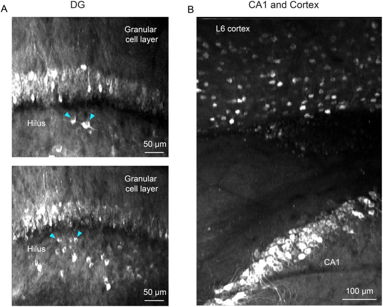
(A) Two maximum projections of imaging planes in which both the granular cell layer and the hilus in the DG could be imaged simultaneously. Example putative mossy cells indicated with cyan arrowheads. Scale bar = 50 μm.
(B) Maximum projection from an imaging session in which both CA1 and L6 of the neocortex are visible, allowing simultaneous imaging of neurons in CA1 and deep layers of the parietal cortex. Scale bar = 100 μm.

(A) Place field width pseudo-colored for each place cell overlaid on the maximum projection from Fig. 5A. Any cell that was not a place cell is not pseudo-colored. Scale bar = 100 μm.
(B) Place field width, as a function of distance along the DG-to-CA1 axis (pCA3 to pCA1), of real data (blue) vs. shuffled control (black). Shaded area is s.e.m. Red lines indicate individual positions with place field values that were outside of the shuffled distribution (p < 0.05). However, a General Linear F-test revealed no significant non-uniformity: F(4, 221) = 1.61, p = 0.17.
SUPPLEMENTAL VIDEOS
Video S1. Demonstration of two-photon imaging of a Slc17a7-GCaMP6s mouse through the microperiscope. Recording starts in the superficial cortex in front of microperiscope, then moves through the microperiscope to the hippocampus, zooming in on subfields CA1, CA3, and DG.
Video S2. Calcium activity in subfield CA1 in a Slc17a7-GCaMP6s mouse imaged through the microperiscope.
Video S3. Calcium activity in subfield DG in a Slc17a7-GCaMP6s mouse imaged through the microperiscope.
Video S4. Mouse running in the floating chamber circular track. Ambient light is higher than usual levels for improved video quality.
METHODS
Animals
For dendritic morphology experiments, Thy1-GFP-M (Jax Stock #007788) transgenic mice (n = 7) were used for sparse expression of GFP throughout the forebrain. For forebrain-wide calcium indicator expression, Emx1-IRES-Cre (Jax Stock #005628) x ROSA-LNL-tTA (Jax Stock #011008) x TITL-GCaMP6s (Jax Stock #024104) triple transgenic mice (n = 2) or Slc17a7-IRES2-Cre (Jax Stock #023527) x TITL2-GC6s-ICL-TTA2 (Jax Stock #031562) double transgenic mice (n = 6) were bred to express GCaMP6s in excitatory neurons. For imaging experiments, 8-51 week old (median 17 weeks) mice of both sexes (6 males and 9 females) were implanted with a head plate and cranial window and imaged starting 2 weeks after recovery from surgical procedures and up to 10 months after microperiscope implantation. The animals were housed on a 12 hr light/dark cycle in cages of up to 5 animals before the implants, and individually after the implants. All animal procedures were approved by the Institutional Animal Care and Use Committee at University of California, Santa Barbara.
Surgical Procedures
All surgeries were conducted under isoflurane anesthesia (3.5% induction, 1.5 - 2.5% maintenance). Prior to incision, the scalp was infiltrated with lidocaine (5 mg kg-1, subcutaneous) for analgesia and meloxicam (2 mg kg-1, subcutaneous) was administered preoperatively to reduce inflammation. Once anesthetized, the scalp overlying the dorsal skull was sanitized and removed. The periosteum was removed with a scalpel and the skull was abraded with a drill burr to improve adhesion of dental acrylic.
For hippocampal imaging, we used two types of custom-designed glass microperiscope (Tower Optical). The first (v1CA1), for imaging the upper part of the hippocampus (CA1/CA2) consisted of a 1 × 1 × 1 mm square base and a 1 mm right angle prism, for a total length of 2 mm on the longest side (Fig. 1B, left). The second (v2HPC), for imaging the entire transverse circuit (CA1-3, DG) had a 1.5 × 1.5 × 1.0 mm (L × W × H) square base and a 1.5 mm right angle prism, for a total length of 2.5 mm on the longest side (Fig. 1B, right). The hypotenuse of the right angle prisms were coated with enhanced aluminum for internal reflectance. The microprism was attached to a 5 mm diameter coverglass (Warner Instruments) with a UV-cured optical adhesive (Norland, NOA61). Prior to implantation, the skull was soaked in sterile saline and the cortical vasculature was inspected to ensure that no major blood vessels crossed the incision site. If the cortical vasculature was suitable, a 3-4 mm craniotomy was made over the implantation site (centered at 2.2 mm posterior, 1.2-1.7 mm lateral to Bregma). For the smaller microperiscope (v1CA1), a 1 mm length anterior-to-posterior incision centered at −2.1 mm posterior, 1.2 mm lateral to Bregma was then made through the dura, cortex, and mediodorsal tip of the hippocampus to a depth of 2.2 mm from the pial surface with a sterilized diamond micro knife (Fine Science Tools, #10100-30) mounted on a manipulator. For the larger microperiscope (v2HPC), two overlapping 1.0 mm length anterior-to-posterior incisions were made centered at −1.8 mm posterior / 1.7 mm lateral and −2.4 mm posterior / 1.7 mm lateral to Bregma to a depth of 2.7 mm, with a total anterior-to-posterior incision length of 1.6 mm. Note that placements in the regions shown in Fig. 1B required incision coordinates slightly posterior to those indicated on the atlas. Care was taken not to sever any major cortical blood vessels. Gelfoam (VWR) soaked in sterile saline was used to remove any blood from the incision site. Once the incision site had no bleeding, the craniotomy was submerged in cold sterile saline, and the microprism was lowered into the cortex using a manipulator, with the imaging face of the prism facing lateral. Once the microprism assembly was completely lowered through the incision until the coverglass was flush with the skull, the edges of the window were sealed with silicon elastomer (Kwik-Sil, World Precision Instruments), then with dental acrylic (C&B-Metabond, Parkell) mixed with black ink. Care was taken that the dental cement did not protrude over the window, as it could potentially scratch the objective lens surface. Given the working distance of the objective used in this study (3 mm), the smaller microperiscope (v1CA1) implant enabled imaging from 2250 - 2600 μm below the coverglass surface, corresponding to approximately 150 - 500 μm into the lateral hippocampus (the 150 μm of tissue nearest to the prism face was not used for imaging). The larger microperiscope (v2HPC) implant enabled imaging from 2650 - 2850 μm below the coverglass surface, corresponding to approximately 150 - 350 μm into the lateral hippocampus (the 150 μm of tissue nearest to the prism face was not used for imaging). The microprism implantations were stable for up to ten months following the surgery.
After microperiscope implantation, a custom-designed stainless steel head plate (eMachineShop.com) was affixed using dental acrylic (C&B-Metabond, Parkell) mixed with black ink. After surgery, mice were administered carprofen (5 - 10 mg kg-1, oral) every 24 hr for 3 days to reduce inflammation. Microperiscope designs and head fixation hardware are available on our institutional lab web site (https://goard.mcdb.ucsb.edu/resources).
Point Spread Function Measurements
To measure empirical point spread functions, fluorescent microspheres (0.2 µm yellow-green fluorescent microspheres; ThermoFisher F8811) were embedded 1:2000 in 0.5% agar and placed under the cranial window or on the face of the microperiscope. Image stacks were taken through the microspheres (0.06 μm per pixel in XY; 0.5 μm per plane in Z), and candidate microspheres were isolated using a watershed algorithm (Matlab image processing toolbox). Only microspheres that were >20 pixels (1.2 μm) away from nearest neighbor microspheres and completely contained within the Z-stack were used for further analysis. We registered isolated microspheres at their centroids and measured the full width at half maximum (FWHM) of the average XY and XZ profiles to determine the lateral and axial resolution, respectively.
Since the geometry of the microperiscope limits the angle of the focusing light cone through the microperiscope, it predominately determines the functional numerical aperture at the imaging plane. Based on the microperiscope geometry, we calculated the effective NA of the v1CA1 microperiscope and v2HPC, and used it to calculate the theoretical lateral and axial resolution according to the following formulae89
 To perform aberration correction with adaptive optics, a deformable mirror (Multi-3.5, Boston Micromachines Corporation) was set at a plane conjugate to the raster scanning mirrors and the back aperture of the objective lens in the two-photon imaging system. Fluorescent microspheres (0.2 μm) were imaged, and the standard deviation of the image brightness was maximized under different configurations of the deformable mirror. Twelve selected Zernike modes are applied and modulated sequentially over a total of three rounds. The 12 zernike modes are: 1) oblique astigmatism, 2) vertical astigmatism, 3) vertical trefoil, 4) vertical coma, 5) horizontal coma, 6) oblique trefoil, 7) oblique quadrafoil, 8) oblique secondary astigmatism, 9) primary spherical, 10) vertical secondary astigmatism, 11) vertical quadrafoil, 12) secondary spherical. For each Zernike mode, 21 steps of amplitudes were scanned through, and images were acquired for each step. The amplitude that resulted in the largest standard deviation was saved and set as the starting point of the DM configuration for the scanning of the next Zernike mode. The brightness, the lateral resolution, and the axial resolution are compared with and without the application of the deformable mirror correction.
Air-floated Chamber
For measurement of spatial responses, mice were head-fixed in a floating carbon fiber chamber34 (Mobile Homecage, NeuroTar, Ltd). The chamber base was embedded with magnets to allow continual tracking of the position and angular displacement of the chamber. Behavioral data was collected via the Mobile HomeCage motion tracking software (NeuroTar, versions 2.2.0.9, 2.2.014, and 2.2.1.0 beta 1). During imaging experiments, image acquisition was triggered using a TTL pulse from the behavioral software to synchronize the timestamps from the 2P imaging and chamber tracking.
A custom carbon fiber arena (250 mm diameter) was lined with four distinct visual patterns (5.7 cm tall, 18.1 cm wide) printed on 7 mil waterproof paper (TerraSlate) with black rectangles (5.7 cm tall and 1.5 cm wide) placed in between the four patterns. A circular track (Fig. 4A; Video S4) was made by adding a removable inner circle (14 cm in diameter and 4.2 cm tall) with visual cues that were matched to the outer wall printed on 7 mil waterproof paper. Transparent tactile stickers (Dragon Grips) were placed on the arena floors to give differential tactile stimuli along the track. In between each recording and or behavioral session, the arena walls and floors were thoroughly cleaned.
Mice were acclimated to the arena by the following steps: 1) On the first day the mice were placed into the chamber and allowed to freely explore without head fixation for 15 - 20 minutes. A piece of plexiglass with holes drilled through was placed on top of the arena to keep the mice from climbing out. 2) On the second day, the mice were head-fixed to a crossbar extending over the floating chamber (Fig. 4A) and allowed to freely explore the floating chamber freely for 15 minutes. Air flow (3 - 6.5 psi) was adjusted to maximize steady walking/running. On subsequent days, the head fixation time was increased by increments of 5 minutes, as long as the mice showed increased distance walked and percent time moving. This was continued until the mice would explore for 30 - 40 minutes and run for greater than 15% of the time. 3) Mice were head-fixed in the floated chamber for 20 minutes with a custom light blocker attached to their headplate. 4) Mice were head-fixed and placed on the 2P microscope to allow habituation to the microscope noise. 5) After mice were fully habituated, 20 - 40 minute duration recording sessions on the 2P microscope were performed.
If at any point during the above acclimation protocol the mouse significantly decreased distance traveled or percentage of time moving, then the mouse was moved back to the previous step.
Custom software was written to process the behavioral data output by the Mobile HomeCage motion tracking software. Because the Mobile HomeCage motion tracking software sampling rate was faster than the frame rate of our 2P imaging, all behavioral variables (speed, location, polar coordinates, and heading) that were captured within the acquisition of a single 2P frame were grouped together and their median value was used in future analysis. For the polar angle (which we used as the location of the mouse in 1D track), the median was computed using an open source circular statistics toolbox (CircStat 2012a) written for Matlab90. We removed any time points when the mouse was not moving, as is standard for measurement of place fields25. This helps separate processes that are related to navigation from those that are related to resting state. To do this, we smoothed the measured instantaneous speed and kept time periods > 1 s that had speeds greater than 20 mm/s (adding an additional 0.5 s buffer on either side of each time period).
Two-photon Imaging
After recovery from surgery and behavioral acclimation, GFP or GCaMP6s fluorescence was imaged using a Prairie Investigator 2P microscopy system with a resonant galvo scanning module (Bruker). For fluorescence excitation, we used a Ti:Sapphire laser (Mai-Tai eHP, Newport) with dispersion compensation (Deep See, Newport) tuned to λ = 920 nm. Laser power ranged from 40-80 mW at the sample depending on GCaMP6s expression levels. Photobleaching was minimal (<1% min-1) for all laser powers used. For collection, we used GaAsP photomultiplier tubes (H10770PA-40, Hamamatsu). A custom stainless-steel light blocker (eMachineShop.com) was mounted to the head plate and interlocked with a tube around the objective to prevent light from the environment from reaching the photomultiplier tubes. For imaging, we used a 16x/0.8 NA microscope objective (Nikon) to collect 760 × 760 pixel frames with field sizes of 829 × 829 μm or 415 × 415 μm. Images were collected at 20 Hz and stored at 10 Hz, averaging two scans for each image to reduce shot noise.
For imaging spines across days, imaging fields on a given recording session were aligned based on the average projection from a reference session, guided by stable structural landmarks such as specific neurons and dendrites. Physical controls were used to ensure precise placement of the head plate, and data acquisition settings were kept consistent across sessions. Images were collected once every day for 5 - 10 days.
Two-photon Post-processing
Images were acquired using PrairieView acquisition software (Bruker) and converted into multi-page TIF files.
For spine imaging, registration and averaging was performed for each z-plane spanning the axial width of the dendrite to ensure all spines were captured across z-planes. The resulting projections were weighted according to a Gaussian distribution across planes. Non-rigid registration was used to align dendritic segments across consecutive recording sessions. The registered images underwent high-pass filtering to extract low amplitude spine features using code adapted from Suite2P’s enhanced mean image function91 (Fig. S2A). The resulting ROIs were binarized using Otsu’s global threshold method for spine classification (Fig. S2A). In most cases, the global threshold successfully isolated the single most prominent dendrite. In fields with higher background dendrites that were not desired, these extraneous dendrites were manually excluded. To identify spines that fall below the global threshold, the user manually specifies incrementally lower thresholds from which to select spines that were excluded in the initial binarization. (Fig. S2A). Spines above the global threshold with an area of >1 μm2 were included in our analysis. To classify each spine as one of the four major morphological classes, we performed the following steps. First, we found the base of the spine by identifying the region closest to the dendritic shaft. Second, we calculated the length of the spine by taking the Euclidean distance between the midpoint of the spine base and the most distant pixel. Third, this vector was divided evenly into three segments to find the spine head, neck, and base areas respectively. Finally, spines were classified in the four categories, considering the following threshold parameters (Fig. S2B): stubby (neck length < 0.2 μm and aspect ratio < 1.3), thin (neck length > 0.2 μm, spine length < 0.7 μm, head circularity < 0.8 μm), mushroom (neck length > 0.2 μm, head circularity > 0.8 μm), and filopodium (neck length > 0.2 μm, spine length < 0.8 μm, aspect ratio >1.3).
For calcium imaging sessions, the TIF files were processed using the Python implementation of Suite2P91. We briefly summarize their pipeline here. First, TIFs in the image stack undergo rigid registration using regularized phase correlations. This involves spatial whitening and then cross-correlating frames. Next, regions of interest (ROIs) are extracted by clustering correlated pixels, where a low-dimensional decomposition is used to reduce the size of the data. The number of ROIs is set automatically from a threshold set on the pixel correlations. We manually checked assigned ROIs based on location, morphology and DF/F traces.
Since the hippocampal pyramidal cells are densely packed and the prism reduces the axial resolution, we perform local neuropil subtraction using custom code (https://github.com/ucsb-goard-lab/two-photon-calcium-post-processing) to avoid neuropil contamination. The corrected fluorescence was estimated according to
 where Fneuropil was defined as the fluorescence in the region <30 μm from the ROI border (excluding other ROIs) for frame n. Fneuropil is Fneuropil averaged over all frames. α was chosen from [0, 1] to minimize the Pearson’s correlation coefficient between Fcorrected and Fneuropil The ΔF/F for each neuron was then calculated as
 where Fn is the corrected fluorescence (Fcorrected) for frame n and F0 is defined as the first mode of the corrected fluorescence density distribution across the entire time series.
We deconvolved this neuropil subtracted ΔF/F to obtain an estimate for the instantaneous spike rate, which we used (only) for the computation of neurons’ spatial information (see below). This inferred spike rate was obtained via a MATLAB implementation of a sparse, nonnegative deconvolution algorithm (OASIS) used for Ca2+ recordings92. We used an auto-regressive model of order 1 for the convolution kernel.
Spine Imaging Data Analysis
After nonrigid registration, high pass filtering, and binarization of the dendritic segment, individual spines were extracted based on standard morphological criteria93. Spines projecting laterally from the dendritic segment were extracted and analyzed as individual objects, as described previously (Fig. S2). The sum of the members of each spine class, as well as the total number of all spines, was recorded for each session. Spine totals (Stotal) were then broken down into 10 μm sections of the dendritic segment (Ssection) using the following calculation:
 where length of the dendritic segment, Dlength, was determined by skeletonizing the dendritic shaft to 1 pixel in diameter, then taking the area of the pixels. Fpixels is the FOV in pixels, which here was 760 × 760 at 16x magnification, and Fµm is the FOV in microns, which was 52 × 52 μm.
Turnover was estimated at 24 h increments; turnover here is defined as the net change in spines per day for each morphological class (Fig. 2F). To determine which specific spines were involved in turnover across days, segments recorded 24 h apart were aligned and overlaid using a custom MATLAB interface, which allowed the user to manually select new or removed spines. Percent addition/subtraction Sa/s was calculated as:
 where Na/s(t) is spines that have been added or subtracted and N(t) is the total average number of spines. To account for variance in spine classification across days, turnover of specific classes of spines was normalized to total cumulative turnover per day.
To calculate the survival fraction curve S(t), we determined which spines were present at time tn that were not present at time t043,44. The dendritic segment from t0 was transparently overlaid with segments from tn, and replacement spines that were present in t0 but not tn were manually identified. Survival fraction was quantified as
 where Nr(tn) are the total spines at tn that were also found in t0, and N(t0) are the total number of spines that were present in t0. Survival fraction, as well as % addition and subtraction, was calculated in 10 μm sections to control for segment length.
Calcium Imaging Data Analysis
For calcium imaging experiments during exploration of the air-floated chamber, processed and synchronized behavioral data and 2P imaging data were used to identify place and speed cells as follows.
First, the 1D track was divided into 72 equal bins (each ∼0.85 cm in length). Activity as a function of position (we refer to these as spatial tuning curves) was computed for each lap, with activity divided by occupancy of each binned location. To avoid misattribution of slow calcium signals to spatial bins, any lap where the average instantaneous speed was greater than 180 mm/s, or where the total length of the lap took less than 1 second, were removed and not considered for further analysis. To assess the consistency of spatial coding of each cell, we randomly split the laps into two groups and computed the correlation coefficient between the averaged spatial tuning curves. We then did the same for shuffled data in which each lap’s spatial tuning curve was circularly permuted by a random number of bins. This was performed 500 times, and the distribution of actual correlation coefficient values was compared to the distribution of circularly shuffled values using a two-sample Kolmogorov-Smirnov test (α = 0.01). A cell that passed this test was considered a “consistent” cell.
To identify a neuron as a place cell, the neuron had to pass the consistency test and also be well fit by a Gaussian function,  , with
  . Specifically, we required that: 1) the adjusted R2 > 0.375; 2) 2.5cm < FWHM < 30.6 cm (50% of rack length); 3) A > 0; 4) A/A0 > 0.50. Cells that met these conditions were characterized as lace cells; with place fields at the location of maximal activity and width defined as the FWHM.
Speed cells were identified using a standard process developed for identification of peed cells in medial enthorinal cortex and hippocampus62–64. We computed the Pearson orrelation of each cells’ DF/F trace with the mouse’s speed across the experiment. This value s considered as a “speed score”. We then circularly shuffled the DF/F 100 times (making sure hat the amount shuffled was greater than 10 frames to ensure that the shuffled distribution did ot have artificially high correlations). Cells whose speed score was greater than 99%, or less han 1%, of the shuffled distribution were considered speed cells.
To compute the spatial information94 of cell j (SIj), we used the following formula
 where āj is the mean inferred spike rate of cell j, aj(k) is the mean inferred spike rate of cell j at position bin k, and p(k) is the probability of being at position bin k. We divide by āj to have SI in units of bits/inferred spike.
To align recordings where we recorded along the CA1-DG axis, we found the inflection point of the axis and then computed the distance of each cell to that point. To do this, we performed the following steps. 1) We extracted the position of each identified cell using Suite2p’s centroid output. 2) We then fit a function of the form a(x – b)2 + c to the cell positions by rotating the field-of-view from 0 to 180 degrees and finding the rotation that maximized the R2 value of the fit. 3) We determined the inflection point as the peak of the curve and de-rotated the fit to determine the inflection point and curve in the original coordinates. The distance of each cell to the inflection point was found by finding the point along the fit curve that had the minimal distance to the cells centroid.
Immunohistochemistry
Samples were perfusion fixed using 4% paraformaldehyde in 0.1M sodium cacodylate buffer (pH = 7.4) for 10 mins, and then immersion fixed overnight at 4°C. Next, sections were rinsed in cold PBS 5 × 5 mins and 1 × 1hr. Whole brains were then embedded in 10% low-melting agarose. Subsequently, 100 μm coronal sections were cut using a vibratome (Leica, Lumberton, NJ). Sections were then blocked overnight in normal donkey serum (Jackson ImmunoResearch; West Grove, PA) diluted 1:20 in PBS containing 0.5% bovine serum albumin, 0.1% Triton-X 100, and 0.1% sodium azide, hereafter, PBTA at 4°C. Next, primary antibodies anti-GFAP (1:500; abcam; ab53554), anti-S100 (1:1000; DAKO; Z0311) were diluted in PBTA and incubated overnight at 4°C. Then, sections were rinsed 5 × 5 mins and 1 × 1hr before corresponding secondary antibodies along with the nuclear stain Hoechst33342 (1:5000; Molecular Probes; H-3570) were incubated overnight at 4°C. Lastly, secondary antibodies were rinsed and sections mounted using Vectashield (Vector laboratories Inc; H-1200) and sealed under #0 coverslips.
High resolution wide-field mosaics of brain samples were then imaged with a 20x oil immersion lens and an Olympus Fluoview 1000 laser scanning confocal microscope (Center Valley, PA) at a pixel array of 800 × 800 and then registered using the bio-image software Imago (Santa Barbara CA).
We then calculated glial cell density as a function of distance from the prism face. First, each mosaic was rotated so that the medial-lateral axis of the brain sample was aligned to be parallel with the horizontal axis of the image. Then each mosaic was cropped to remove extraneous pixels outside of the imaged brain slice. Next, a line denoting the face of the prism was manually drawn parallel to the dorsal-ventral axis aligned with the location of the prism face. We then used a custom cell-counting algorithm that identified potential regions of interest (ROIs). We limited the ROIs to be within the hippocampal formation in the brain slices. The euclidean distance between the closest point on the defined prism face and each ROI’s centroid was calculated. Afterward, a similar procedure was performed on the contralateral side of the brain slice, with a mock “prism face” defined at symmetric coordinates to the true prism face, to serve as a control. These steps were repeated for each channel of the mosaic.
After extracting each ROIs distance from the prism face, we counted the number of cells in each 50 µm distance bin. To account for basal glial cell density, we calculated the percent change of glial cell density on the prism side with respect to the control side. This procedure was repeated 1000 times using randomly sampled distances, with replacement, to bootstrap the sample variance.
Statistical Information
Violin plots were made using an open source Matlab package95. Statistical tests for spine morphological types were calculated using a one-way ANOVA. Reliability across laps was tested with a two-sample Kolmogorov-Smirnov test. Comparisons between model fits for spatial distribution of spatial information and place field width used a General Linear F-test.
DATA AVAILABILITY
Microperiscope designs can be found on our institutional lab website (https://goard.mcdb.ucsb.edu/resources). Spine imaging data from Fig. 2 and neuronal response data from Figs. 4-5 are available on Dryad (DOI: TBA, final version will be uploaded upon manuscript acceptance). Code for spine analysis and place/speed cell identification is available on Github (DOI: TBA, final version will be uploaded upon manuscript acceptance).
AUTHOR CONTRIBUTIONS
W.T.R. and M.J.G. designed the experiments; M.J.G. performed the surgical implants; W.T.R., N.S.W., L.M., and M.J.G. conducted the imaging experiments and analyzed the data; G.L. and T.D.M. performed immunohistochemistry and K.K.S. analyzed the resulting images; C.H.Y. and S.L.C. performed optical modeling; W.T.R., N.S.W., and M.J.G. wrote the manuscript.
COMPETING INTERESTS
The authors declare no competing financial interests.
MATERIALS AND CORRESPONDENCE
Correspondence and material requests should be directed to michael.goard{at}lifesci.ucsb.edu.
ACKNOWLEDGEMENTS
We would like to thank Caleb Kamere and Eliott Levy for comments on the manuscript. This work was supported by NSF (M.J.G., S.L.S., NeuroNex #1707287), NIH (M.J.G., S.L.S., R01NS121919), the Whitehall Foundation (M.J.G.), and the Larry Hillblom foundation (M.J.G.).
REFERENCES
- 1.↵
- 2.
- 3.↵
- 4.↵
- 5.↵
- 6.
- 7.↵
- 8.
- 9.↵
- 10.
- 11.
- 12.
- 13.↵
- 14.↵
- 15.↵
- 16.
- 17.
- 18.
- 19.↵
- 20.↵
- 21.↵
- 22.↵
- 23.↵
- 24.↵
- 25.↵
- 26.↵
- 27.↵
- 28.↵
- 29.↵
- 30.↵
- 31.↵
- 32.↵
- 33.↵
- 34.↵
- 35.↵
- 36.↵
- 37.
- 38.↵
- 39.↵
- 40.↵
- 41.↵
- 42.↵
- 43.↵
- 44.↵
- 45.↵
- 46.↵
- 47.
- 48.↵
- 49.↵
- 50.↵
- 51.↵
- 52.↵
- 53.↵
- 54.
- 55.↵
- 56.↵
- 57.↵
- 58.↵
- 59.↵
- 60.↵
- 61.↵
- 62.↵
- 63.↵
- 64.↵
- 65.↵
- 66.
- 67.
- 68.
- 69.↵
- 70.↵
- 71.↵
- 72.↵
- 73.↵
- 74.↵
- 75.
- 76.↵
- 77.↵
- 78.
- 79.
- 80.
- 81.↵
- 82.↵
- 83.
- 84.↵
- 85.↵
- 86.↵
- 87.↵
- 88.↵
- 89.↵
- 90.↵
- 91.↵
- 92.↵
- 93.↵
- 94.↵
- 95.↵


