

Abstract
Gastrulation is a critical event in vertebrate morphogenesis driven by cellular processes, and characterized by coordinated multi-cellular movements that form the robust morphological structures. How these structures emerge in a developing organism and vary across vertebrates remains unclear. Inspired by experiments on the chick, we derive a theoretical framework that couples actomyosin activity to tissue flow, and provides a basis for the dynamics of gastrulation morphologies. Our model predicts the onset and development of observed experimental patterns of wild-type and perturbations of chick gastrulation as a spontaneous instability of a uniform state. Varying the initial conditions and a parameter in our model, allows us to recapitulate the phase space of gastrulation morphologies seen across vertebrates, consistent with experimental observations in the accompanying paper. All together, this suggests that early embryonic self-organization follows from a minimal predictive theory of active mechano-sensitive flows.
Gastrulation is an essential, highly conserved process in the development of all vertebrate embryos (1), with the chick being an extensively studied model because it is easily cultured and imaged. During gastrulation, the chick transforms from a layer of epithelial cells into a layered structure of three major embryonic tissues, the ectoderm, mesoderm and endoderm. At the moment of egg-laying, the chick embryo contains around 60,000 cells organized in a central concentric epiblast that will give rise to the embryo proper (EP) surrounded by a ring of extraembryonic (EE) tissue. During the first few hours of development, signals from the extraembryonic tissues, the epiblast and the developing hypoblast induce mesendoderm precursor cells located in a sickle-shaped domain at the posterior edge of the epiblast (2) (Fig. 1A). These mesendoderm precursor cells start to execute directed cell intercalations that results in a contraction of the mesendoderm tissue towards the central midline followed by an extension in anterior direction, forming the primitive streak (PS) (3,4) (Figs. 1A-B). In the streak, the mesendoderm precursor cells undergo an epithelial to mesenchymal transition; they ingress individually and migrate away to form the various meso and endodermal structures and organs (5, 6). This directional cell intercalation process drives embryo scale counter-rotating tissue flows in the epiblast merging at the site of the formation of the PS (7, 8) (Fig. 1B).
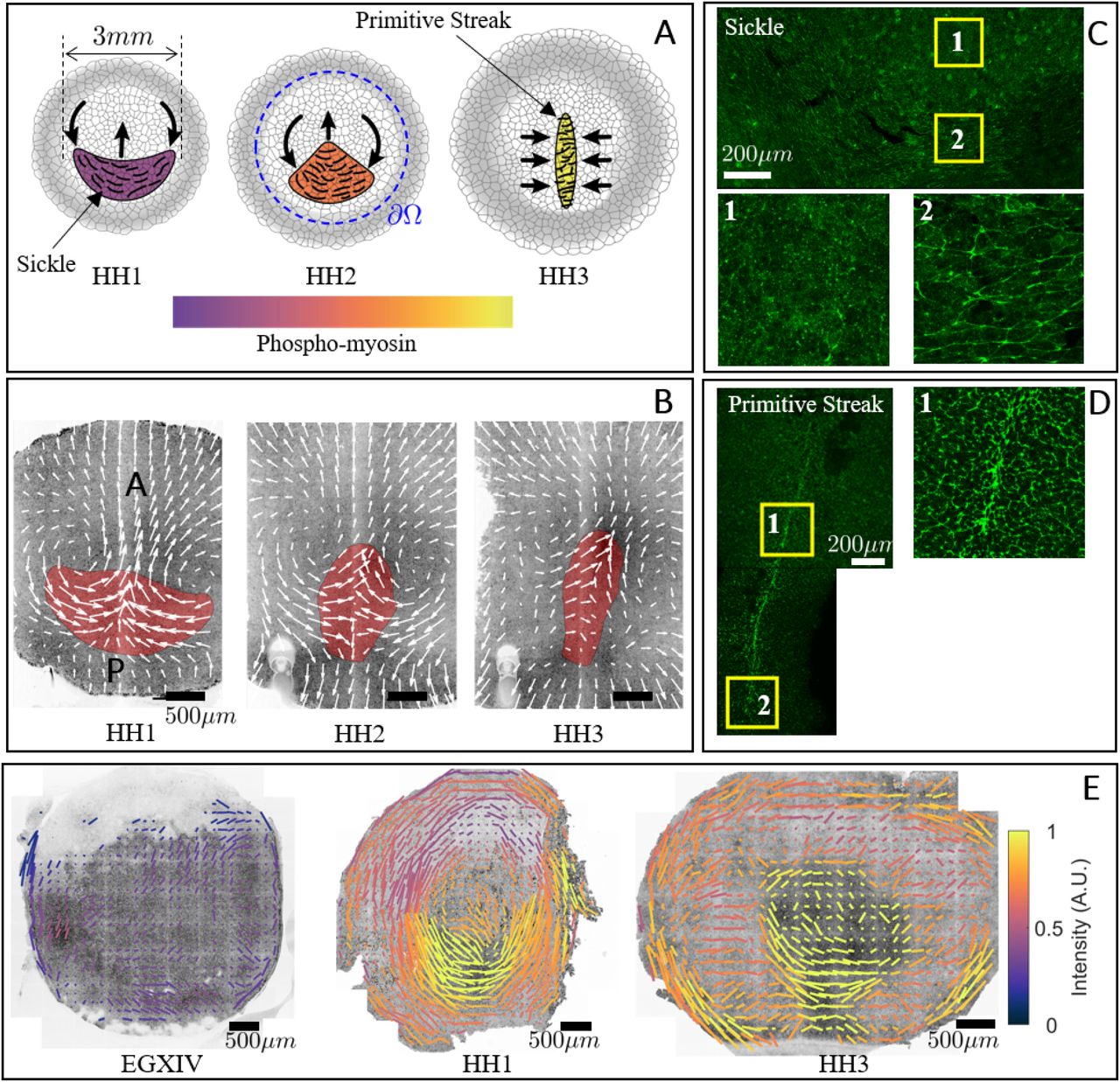
A) Diagram of the formation of the PS. B) Formation of the PS on a chick gastrula. The convergent extension of the mesendoderm (red) originate macroscopic tissue flows on the surface of the embryo. C) The mesendoderm sickle territory is characterised by supracellular cables of active myosin (phospho-myosin light chain, pMLC) perpendicular to the anterior-posterior (AP) direction. The PS is characterised by supracellular cables of active myosin (pMLC) perpendicular to the midline. E) The pattern of actomyosin cables evolves over time. The bars represent the pMLC anisotropy and the color of the bars indicates the relative concentration. For details see the accompanying paper (9).
There are three cellular scale active force-generating processes that drive tissue flows: (i) the outward migration of the cells attached to the vitelline membrane at the boundary of the embryo, (ii) the active intercalation of the mesendoderm precursors generating forces in the plane of the epiblast, (iii) the ingression of mesendoderm cells in the streak, wich attracts cells towards the streak and drives the out of plane motion. It is likely that the variation of tissue flows and morphologies seen during gastrulation across vertebrates, ranging from fish and amphibians via reptiles to amniotes such as chick and human, are due to changes in the embryo geometry and the relative contribution of these three force-generating processes.
At the cellular level, in the chick, the onset of directional intercalation correlates with the appearance of oriented chains of aligned junctions containing active actomyosin, as detected by phosphorylation of the myosin light chain (4, 10) (Figs. 1A left, C). This indicates the appearance of a supra-cellular oriented organization (planar cell polarity) of intercalating cells (SFig. 4). During the extension of the primitive streak the supracellular cables of highly active myosin reorient to become perpendicular to the midline (Figs. 1A right, D, E). These myosin cables, first observed in directional cell intercalation underlying germband extension in fruitfly embryogenesis (11, 12), were thought to arise from signaling in the anterior-posterior patterning system (13). More recent work (14) suggests instead that the myosin cables could self-organize in a tension-dependent manner, and thus lead to spontaneous large-scale orientation during PS formation. Consistent with this, it is now well established that cytoskeletal actin dynamics, myosin activity and adhesion, are mechano-sensitive (15), e.g. contraction of a given junction will increase its tension, which in turn activates the myosin assembly and further myosin recruitment through a catch-bound mechanism (16–18) (Fig. 2A). This positive feedback mechanism could then result in the formation of supra-cellular chains of myosin-enriched junctions at the cellular level that drive coordinated supra-cellular directional intercalation, organized tissue flow and PS formation (2). In the chick, the early embryonic layer can be abstracted as a thin two-dimensional fluid in which myosin activity leads to active stresses which induce multicellular flows. Interfering with myosin activity correlates with the failure of PS formation (4) and accompanying paper (9). But what are the essential mechanisms sufficient to generate supra-cellular coordination?

A) High tension T along actomyosin cables induces additional myosin recruitment via the catch-dynamics, further increasing T. This positive feedback process causes the instability of eq. (1). B) 1D Model recapitulates a focusing-type instability of active myosin, which induces a co-located velocity sink describing cell ingression at the PS. Movie1 shows the time evolution of m, u, ux. C) Initial (t0) and final (tf) distributions of m, ϕ for the 2D model. The instability of m drives the redistribution of cables orientation generating compression (tension) at the P (A) PS. D) Model-based DOA at t0 and the attractor at tf. Movie2 shows the time evolution of the relevant model-based Eulerian and Lagrangian fields. E) Same as D from the experimental velocity. Movie3 shows the time evolution of the Lagrangian metrics from the experimental v. The colorbar in E shows attraction rates in min−1. See materials and methods for values of parameters and boundary conditions used in simulating Eq. (1).

Changes in a critical morphogenetic parameter p0 (the isotropic to anisotropic active stress ratio and regulates the amount of active cell ingression and EMT) and in the initial conditions m(t0) (the extent of the mesendoderm precursor territory) recapitulate major evolutionary transitions of vertebrate gastrulation, as reproduced experimentally in the chick embryo (see accompanying paper (9)). The right columns show deformed Lagrangian grids overlaid to the light-sheet microscope fields (9) and the attractors from Figs. 2-3 associated with different gastrulation modes. Scale bars are 500 μm.
To probe the conditions for the emergence and self-organization of ordered active myosin cables during development and correlate these with observed tissue flows in normal and perturbed conditions, we need a quantitative predictive model. Minimally, a planar mechanochemical model of PS formation during gastrulation should couple three coarse-grained fields: the tissue velocity field v(x, y, t) = (u(x, y, t), v(x, y, t))T, the active stress intensity m(x, y, t) arising from the active myosin, and the cable orientation ϕ(x, y, t). In the limit of slow viscously-dominated flows associated with morphogenesis, we can neglect inertia so that local force balance reads ∇ · σT = 0, where the total stress σT = σV + σA is the sum of the viscous stress σV = pI + 2μSs (μ being the shear viscosity and Ss = (∇v + ∇vT – (∇ · v)I)/2 the deviatoric rate-of-strain tensor), and the active stress  , where B = e ⨂ e characterizes the local stress tensor associated with the contractile myosin cables whose orientation vector is given by e = (cos ϕ, sin ϕ)T.
Our model of the sheet-like embryo is assumed to be a compressible fluid to accommodate cell ingression. This implies that we need a continuity law that accounts for flow divergence (or convergence). A simple linear model for this is ∇ · v = c (Trace[σT] – p0m). Here c−1 is the fluid bulk viscosity while p0 characterizes the effect of active cell ingression and can be thought of as the ratio between the isotropic to anisotropic active stress (see material and methods for a detailed description and the implications of this law), and reflects the expectation that both the average compressive stress and active myosin contribute to negative divergence and thence cell ingression. Then, we may write the equations for local momentum balance for the planar velocity field v(x, y, t), along with equations for the orientational ϕ(x, y, t) and intensity m(x, y, t) dynamics of myosin cables as

Here we have nondimensionalized our model using the characteristic length scale xc, speed uc and viscous shear stress μuc/xc. In the first equation in (1), the first two terms are the contributions from shear and dilatational deformations, the last three terms are a consequence of active forces induced by inhomogeneities in the myosin concentration and cable orientation, while p1 = μc is the ratio of the shear viscosity to the bulk viscosity (see materials and methods § 1-2 for a derivation of these equations). The second equation in (1) describes the orientational dynamics of myosin cables which evolve like material fibers, advected by the flow and rotated by vorticity ω and shear (19), with the non-dimensional parameter p2 ∼ O(1) for elongated fibers. The last equation tracks the magnitude of the active stress intensity associated with the recruitment of myosin from the cytoplasm, assumed to have a uniform constant concentration mn, at scaled rate  (here tp is the phosphorylation time scale for converting active myosin into active stress and tr is the recruitment time scale). The second term on the right of the last equation is associated with the positive feedback induced by the catch-bond dynamics in loaded cables (Fig. 2A) that has an exponential form (20) (with m/2 being the cable tension and
  is the ratio of the characteristic shear stress of the system to the characteristic bonding stress between actin and myosin).
  is the ratio of phosphorylation time scale to the dissociation time scale, and the last term accounts for myosin diffusion with
  being the inverse of the Peclet number characterizing the ratio between diffusive and advective transport of myosin. Given the circular geometry of the embryo, we solve our model in polar coordinates (see materials and methods for a detailed derivation, nondimensionalization, discussion and numerical scheme). We consider a spatial domain with boundary ∂Ω (Fig. 1A) that encloses the embryonic area and a small fraction of the EE region. This allows us to keep the size of the domain approximately fixed, as the embryonic area remains constant. To complete the formulation of the problem, we need boundary and initial conditions. For boundary conditions, we impose the epiboly velocity and no flux for m, ϕ, i.e. v = vb|∂Ω, ∇m · n = 0, ∇ϕ · n = 0, with n being the outer normal to ∂Ω. See materials and methods for the selection of the parameters in our simulations.
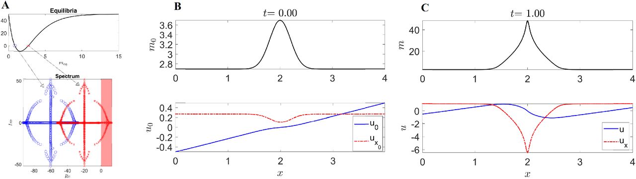
To gain intuition, we derive and analyze (materials and methods) the 1D version of eq. (1) modeling the dynamics perpendicular to AP, as summarized in Fig. 2B. Linear stability analysis of uniform equilibria of m reveals that the (lower) higher equilibrium is linearly (stable) unstable (SFig. 2). Initializing the nonlinear system with a Gaussian perturbation m(t0) to the unstable equilibrium (mimicking the onset of actomyosin cables in the sickle as in Figs.1A,C), our model develops a focusing-type instability which significantly increases m(tf) while generating a highly compressive region ux(tf) ≪ 0, reproducing cell ingression at the streak. Movie1 shows the time evolution of the relevant fields. While the simplified 1D model neglects the orientation of the cables, it accounts for the catch-bond dynamics coupled with the flow field and our continuity law, both of which carry over the full model.
To quantify the global nature of the self-organized spatio-temporal patterns, we use the notion of Lagrangian coherent structures adapted to morphogenetic flows, i.e. their dynamic morphoskeletons (DM) (21). The DM is based on a Lagrangian description of tissue deformation captured by the Finite Time Lyapunov Exponents (FTLE), which naturally combines local and global mechanisms along cell paths. The DM consists of attractors and repellers toward which cells converge or diverge over a specific time interval T = tf – t0. Repellers are marked by high values of the forward  ; attractors are marked by high values of backward
  and their domain of attraction (DOA) by high values of the backward FTLE displayed on the initial cell positions
  (see materials and methods for details).
We initialize the 2D model with a curved Gaussian perturbation (mimicking the mesendoderm precursor) to the unstable equilibrium of m and ϕ(t0) in the azimuthal direction (Fig. 2C), consistent with experiments (Fig. 1E and Fig. 3 of (9)). The instability of m drives both the flow velocity and the orientation of the cables shown in Fig. 2C and Movie2, reproducing the typical flow patterns observed in wild-type experiments. A closer look at m, ϕ shows that the active stress resulting from our self-organizing model induces tension in the anterior and compression in the posterior (red arrows Fig. 2C), resembling the stress distribution on the tensile ring observed in (10). While (10) imposes the tensile ring on a fixed circle located at the boundary between the EP and EE area, our active stress distribution arises spontaneously from Eq. (1) and evolves dynamically in space. This is consistent with our experimental results where we identify the EP-EE boundary as a repeller (21) and track its spatio-temporal evolution (SFig. 5 and SM Movie1). Figures 2D-E show the DOA (left) and the attractor (right), corresponding to the largest T obtained from both the model and the experimental v. The attractor marks the formed PS, while the DOA marks the initial position of cells that will form the PS (see Movie2 for the time evolution of the model-based m, ϕ, v, attractors, repellers and a deforming Lagrangian grid as T increases, and Movie3 for the same Lagrangian quantities obtained from the experimental velocity fields). These results complement Fig. 1A-G and Movie1 of (9) showing brightfield images and gene expression patterns that indicate the cable orientation and myosin concentration, consistent with our model. All together, a comparison of the model- and experiment-based Lagrangian metrics shows that our model accurately explains the appearance of the localized zone of myosin activity and the concomitant flows as a spontaneous instability that leads to a self-organized dynamical structure, in contrast to its imposition at a fixed location between the EP and EE in earlier work (10).

A-B) Spontaneous twin perturbation. A) Model-based repeller and attractor for the largest T. Movie4 shows the time evolution of the relevant model-based Eulerian and Lagrangian metrics. B) Same as A from the experimental v. Movie5 shows the time evolution of the Lagrangian metrics from the experimental v. C-D) Inhibition of cell ingression at the PS. C) Model-based DOA and attractor for the largest T. Movie6 shows the time evolution of the relevant model-based Eulerian and Lagrangian metrics. D) Same as C from the experimental Movie7 shows the time evolution of the Lagrangian metrics from the experimental v. E-F) FGF2 addition provokes a circular PS. E) shows the same as C. Movie8 shows the same as Movie7. F) and Movie9 are the same as E and Movie8 from the experimental v. G-H) BMP and GSK3 induce a ring-shaped mesoderm territory at the EE-EP interface while blocking apical contraction and cell ingression in the PS. G) shows the same as C. Movie11 shows the same as Movie7. H) and Movie12 are the same as G and Movie11 from the experimental v. Colorbars in experimental panels show attraction rates in min−1. See materials and methods for values of parameters and boundary conditions used in simulating Eq. (1).
To further test the predictive power of our model, we move beyond gastrulation in wild-type avian embryos, and introduce four different perturbations that modify either the initial state of the embryonic pattern (e.g. its mesoderm) or the active cell ingression encoded in p0. Occasionally, a natural event corresponding to the spontaneous formation of twins arises when the mesendoderm precursor area is split in two regions, from which two streaks emerge. These streaks interact through their tissue flows and form complete or partially twined embryos (Figs. 3A-B). We initialize our model as in the wild type (Fig. 2C) but adding two distant Gaussians to the uniform unstable equilibrium of m. Movie4 shows the model-based Eulerian fields and the induced Lagrangian metrics for increasing T. Figure 3A shows the model-based repeller and the attractor for the largest T. The circular repeller separates the EP from the EE region as well as the AP regions of the PS, while the attractor marks the merging PSs. Figure 3B and Movie5 show the same as 3A and Movie 4 for the experimental v. Comparison of Movie 4 and 5 highlights how our model recapitulates the full morphogenetic process quantified clearly by the DM.
In the second perturbation, we interfere with a signalling pathway via application of the VEGF receptor (Vascular Epithelial Growth Factor) inhibitor Axitinib (100nM), which results in an strong inhibition of ingression of cells in the streak (Figs. 3C-D). We initialize our model as in the wild type (Fig. 2C) but set p0 = 0 as Axitinib prevents active cell ingression. Figures 3C-D show the DOA and attractor for both the model and experimental v, highlighting how this perturbation results in a shorter and thicker PS as well as a reduced amount of ingressed cells, consistent with the results shown in Fig. 2H-N and Movie6 of (9). Movie6 and Movie7 show the time evolution of the model- and experiment-based fields confirming a strikingly similar DM again. The third perturbation consists of FGF2 addition which provokes the generation of a mesoderm ring along the marginal zone that essentially behaves like a circular PS. For this case, we use the same conditions of the wild type, but set m(t0) as a circular ring added to the unstable equilibrium (see m(t0) in Movie8). Figures 3E-F show the DOA and attractor corresponding to the largest T from the model and experimental v, highlighting a sharp circular PS. Movie8 and Movie9 show the Eulerian fields and the Lagrangian metrics for increasing T, while Movie10 shows a deforming Lagrangian grid overlaid on the light-sheet microscope images. These results complement those in Fig. 1H-N of (9) and confirm the predictive power of our model. As the last perturbation, we induce the formation of mesoderm with a combination of the BMP (Bone Morphogenetic Protein) receptor inhibitor LDN – 193189 (100nM) and the GSK3 (Glycogen Synthase Kinase 3) inhibitor CHIR – 99021 (3μM). This induces a ring shaped mesoderm territory at the EE-EP interface. This treatment furthermore blocks apical contraction and cell ingression in the PS, but has little effect on cell intercalations, resulting in the buckling of the tissue (Fig. 2A-G and Movie 5 of (9)). In our model, we use the same setting of perturbation 3 but set p0 = 0 following the same reasoning of perturbation 2. Figures 3G-H show the DOA and the attractor for to the largest T from the model and the experimental v, while Movie11 and Movie12 display the corresponding time evolution of the Eulerian fields and Lagrangian metrics.
To go beyond studying the gastrulation modes in wild-type avian embryos exemplified by the chick, in the accompanying paper (9) we used chemical inhibitors to uncouple cell intercalation and ingression and perturb the initial patterning and function of the prospective mesendoderm. Our results show that we can recapitulate some of the major evolutionary transitions in the morphodynamics of vertebrate gastrulation. The current paper complements this in terms of a mechanochemical model that couples the dynamics of actomyosin cables to large-scale tissue flow patterns. By changing the isotropic to anisotropic active stress ratio, characterized by the parameter p0, together with the initial prospective mesendoderm, described by m(t0), (Fig. 4 left), we can capture the observed variations in the modes of vertebrate gastrulation (Fig. 4 center, right). Specifically, the PS structures in Figs. 3 C-D resemble the blastoporal groove observed in reptilian gastrulation, the circular streak structure (Figs. 3 E-F) resembles the germband of teleost fish gastrulation, while the buckling tissue in Figs. 3 G-H mimics the tissue organization and flow during the closing blastopore in amphibians. Altogether, these results suggest that a relatively small number of changes in critical cell behaviors associated with different force-generating processes leads to distinct vertebrate gastrulation modes via a self-organizing process that might be relatively easily evolvable.
Supplementary Materials for
1 Mathematical Model
We derive our model in Cartesian coordinates first, and then provide an equivalent reformulation in polar coordinates.
1.1 Model in Cartesian coordinates
We denote the cell velocity field by v(x, t) = [u(x, t), v(x, t)]T, its vorticity scalar by ω(x, t), and we recall the velocity gradient decomposition
 with the rate-of-strain tensor S and the spin tensor W defined as

We further decompose S into its isotropic and deviatoric parts as

The viscous, active, total stresses and total stress trace are
 where μ denotes the shear viscosity, m denotes the stress magnitude arising from the active myosin concentration and ϕ the orientation of the myosin cables with respect to the x – axis. The active stresses tensor σA has eigenvalues ± m/2 and eigenvectors {e, Re}. In our model, a cell can be thought of as two springs in parallel: one representing the actomyosin cables that exert the active stress, and the second one representing the rest of the cell exerting the viscous stress. Therefore, the actomyosin cables tension can be computed as

It is known that actin and myosin are characterized by catch bonds (1), i.e. that the dissociation rate of acto-myosin bonds depends on the tension along the actomyosin cable Tc, and decreases exponentially for increasing tension. Using this assumption and eq. (S5), we model the evolution of active stress magnitude as
 where tr is the recruitment time scale of myosin from the cytoplasm, which has a given constant concentration mn, and
  represents the tension-dependent dissociation rate of actomyosin cables. Note again that m, mn have units [Pa] as they describe the stress magnitude arising from active myosin. From the time when active myosin is available to the time it generates active stresses, there is a time scale associated with the phosphorylation process (tp). We model this delay with the ratio (tp/tc), where tc is the characteristic time scale of the system. Finally, the last two terms represent the advection term and the diffusion of active stress magnitude with diffusivity D.
We assume the evolution of actomyosin cables orientation satisfies Jeffery’s equation (2)
 which describe the direction evolution of axis-symmetric fibers under the influence of a low Reynold’s number flow. In eq. (S7),
  is a parameter quantifying the sensitivity of actomyosin cables reorientation due to shear-induced rotations, Sij denotes the entries of S and the last two terms represent the advection term and the rigid-body rotation rate described by half of the flow vorticity.
Because viscosity is high (μ ≈ 9 × 10³ Pa · s), we ignore inertial terms and write the momentum balance as

To close the system, we choose a simple continuity equation in which the flow divergence is proportional to the average total stress (eq. (S4)) and active myosin concentration as
 where c has units [Pa · s]−1 and p0 is a non-dimensional parameter modulating the contribution of active myosin to flow divergence and can be thought of as the ratio between the isotropic to anisotropic active stress. The intuition behind eq. (S9) is that regions of high compressive stress (averaged over all directions) and high active myosin exhibit negative flow divergence, i.e. cell ingression. Substituting eq. (S9) into eq. (S8), we obtain the resulting PDEs describing our active continuum without pressure terms

1.1.1 Non-dimensional model in Cartesian coordinates
Denoting by uc, xc, tc = xc/uc and mc = μuc/xc the characteristic velocity, characteristic length scale, characteristic time scale and the characteristic viscous shear stress, we rewrite eq. (S10) in non-dimensional compact form as
 where m, ϕ, u, v, x, y, t are nondimensional. In eq. (S11), there are seven nondimensional parameters

p0 describes the ratio of isotropic to anisotropic active stresses, p1 describes the ratio of the shear to bulk viscosity, p2 ∈ [0, 1] is the alignment parameter that describes how the actomyosin cables tend to orient due to shear-induced rotations, p3 represents the ratio of the myosin recruitment time scale (from the ambient myosin pool of concentration mn/mc) to the characteristic phosphorylation time scale, multiplied by mn/mc. p4 represents the ratio of the myosin phosphorylation time scale to the dissociation time scale. p5 is the product of the characteristic viscous shear stress and ko, which represents the inverse of the characteristic tension of the actomyosin cables (with units [Pa]−1). p6 is the inverse of the Peclet number characterizing the ratio between diffusive and advective transport of the active stress magnitude.
The first two terms of the force balance are a viscous force and a force arising from compressibility inhomogeneities. Instead, the last three terms are active forces induced by m and ϕ inhomogeneities. To gain insights on p0, we rewrite the force balance as

Assuming a uniform ridge of active myosin in the y direction, cables parallel to the ridge as in the case of perturbation 3 (Fig. 3E-F and Fig. 3 of (3), and neglecting the last two terms, we can see how p0 affects the relationship between the gradient of myosin and the one of the velocity divergence (SFig. 1). Specifically, when the isotropic to anisotropic active stress ratio p0 > 1, a ridge of high myosin induces a sink in the velocity field. By contrast, p0 < 1 induces a source. Comparing our reasoning with experimental observations (Fig. 1L and Fig. 3 of (3)), in our model we use p0 > 1 or p0 = 0.

We consider only the first three terms of eq. (S13) and a simple distribution m made of a ridge in the y direction with actomyosin cables parallel to the ridge.
Finally, observing the first two terms in the last equation in (S11), we note that more myosin induces higher tension on the cables, which in turn decreases the dissociation rate: (m ↑) → Tc ↑ (more positive) → diss. rate ↓ → myosin increases (m ↑) (Fig. 2A). This observation suggests an instability, which will become clear in the next section.
1.1.2 One-dimensional model in Cartesian coordinates
To gain insights about model (S11), we assume slow dynamics in the y– direction, ignore the ϕ–dynamics and set ϕ = 0, obtaining the following simplified one-dimensional model

Because in 1D there is no difference between isotropic and anisotropic stress, we set p0 = 0 without altering the relevant properties of our simplified model. Equation (S14) describes the dynamics along a straight line perpendicular to the primitive streak. We set Dirichlet boundary conditions on the velocity u(0, t) = |ub|, u(L, t) = |ub| consistent with the symmetric cell migration in the extra-embryonic area, and no-flux boundary conditions for m: mx(0, t) = mx(L, t) = 0.
We investigate the main features of eq. (S14) by seeking the constant fixed points for m which solve the implicit equation  . From the first equation, we compute the corresponding equilibrium velocity field
  . We then study the linear stability of these equilibrium solutions by computing the spectrum of the corresponding linearized PDE. Denoting by δh = [δu, δm]T the perturbation from the equilibrium, we compute the linearized version of Eq. (S14) in operator form as 𝒜δh = (x)δh where
 whose boundary conditions are inherited from the nonlinear problem, and correspond to zero Dirichlet boundary conditions for δu and zero flux boundary conditions for δm. We discretize the linearized PDE using a centered finite differencing scheme (4) and compute the generalized eigenvalue problem associated with eq. (S15).

(A) Top: Graph of  shows two meq. marked with a blue circle and a red asterisk. Bottom: Truncated spectrum of the linearized PDE around meq., ueq., consisting of the 500 eigenvalues with the highest real part. (B) Initial condition of the nonlinear 1D model using as initial myosin concentration a Gaussian added to the higher unstable meq.. The blue curve shows the associated initial velocity u0, and the red dashed curve the initial velocity divergence
  . (C) Same as B at the final time. The full time evolution is available as Movie 1. Parameters: p0 = 0, p1 = 0.25, p3 = 100, p4 = 100, p5 = 1.25, p6 = 0.001, ub = 0.5, L = 4, dx = 0.008, dt = 0.0001.
Supplementary Figure 2A top shows two constant equilibria meq., while the bottom panel shows the corresponding 500 eigenvalues with the largest real part of the linearized operator for both the equilibria. The spectrum suggests that the low (high) myosin concentration is linearly stable (unstable) for the chosen parameter values. We confirm these linearized results by solving the full nonlinear PDE from an initial Gaussian myosin distribution added to the unstable meq. (SFig. 2B top). From a biological perspective, a region of higher m0 represents the mesendoderm precursor. At later times (SFig. 2C), m undergoes a focusing instability, that in turn generates a 1D attractor corresponding to the PS and marked by a peak of negative divergence (red dashed curve). The complete time evolution is available as Movie 1. Finally, the velocity divergence ux shows a contracting region close to the PS as well as two symmetric expanding regions close to the boundary, consistent with the isotropic deformations observed in the Embryonic and Extra-Embryonic territories (5). Our simple 1D model reproduces several key features of amniote gastrulation and perhaps elucidates some of its hidden driving mechanisms. Yet, it is insufficient to reproduce the convergent extension and vortical patterns observed in experiments, which we investigate with our 2D model.
1.2 Model in polar coordinates
Because of the circular geometry of the Extra-embryonic tissue as well as the symmetric radial cellular motion at its outer boundary, we re-derive our model (S10) in polar coordinates.

Illustration of the discretization grid (first quadrant) used to solve eq. (S17). β denotes the cables orientation relative to α.
Denoting the velocity field by v = u(r, α, t)er + v(r, α, t)eα and the cables orientation relative to α by β (SFig. 3), we obtain
 which, in non-dimensional form, becomes

2 Parameters
In our simulations, we select the parameter values as follows. p0 = 0 when active cell ingression is inhibited with drugs and p0 = 2 otherwise. We set p1 = 0.15 and note that increasing p1 models a more compressible tissue. With higher p1, the typical counter-rotating vortices (polonaise movement) disappear due to increased cell ingression and less cell redistribution. We set p2 = 0.9 as we model actomyosin cables as elongated passive fibers. To get the order of magnitude of p3, p4, we note that the phosphorylation time scale (tp) to generate active stress from active myosin is ≈ 20min, while the recruitment and dissociation time scales tr ≃ td ≈ 10s. With these estimates, we set p3 = 50 and p4 = 100. We are unaware of techniques to estimate p5, and set p5 = 1.25. We find, however, that slight variations in p3, p4, p5 do not alter the overall system behavior as long as the topology of the graph (SFig. 2A) determining meq. does not change significantly. We set p6 = 0.001 and note that its variations have negligible effects on our results. Finally, because ∂Ω (Fig. 1A) is close to the EP-EE boundary, where the normal velocity is zero, we set |vb| = 0.1. Slight changes in |vb| do not affect the qualitative behavior of our results. We summarize our parameters in table 1.
Parameter values.
Overall, we have selected parameter values using a combination of mechanistic arguments and numerical tests. A detailed analysis of the parameter space is planned for future work.
3 Numerical Scheme
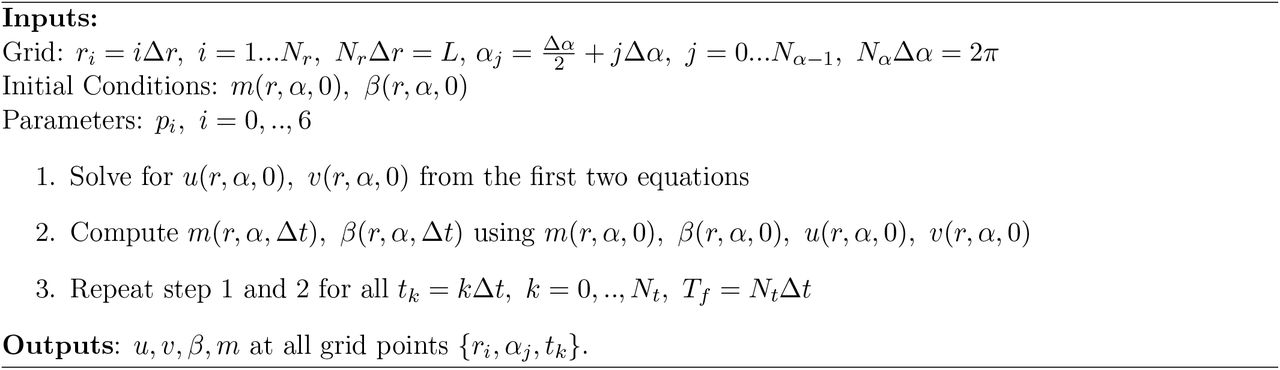
We develop a finite-difference numerical scheme to solve eq. (S17) in MATLAB. First, we multiply the momentum balance equations by r2, leaving their solutions unaltered while avoiding numerical issues at grid points close to the origin. Then, we discretize spatial differential operators using centered finite-difference at second-order accuracy, except at the grid points (r1, αj) (SFig. 3), where we use forward finite-difference at second-order accuracy (4). We solve the first two equations for u, v by inverting (once) the corresponding discretized differential operator, which we multiply at each time step to the discretized forcing vector arising from the updated β, m-dependent terms. We adopt a two-step Adams–Bashforth method to solve the last two PDEs for β and α.
Because the cables orientation is a direction instead of a vector field, spatial derivatives of β care. Specifically, when computing  , one should make sure that both the sign and the amplitude are correct. We do so by rewriting
  , where
  , and compute
  arccos ⟨eβ(i+1,j), eβ(i,j)⟩, where eβ = [cos β, sin β, 0],
  The same strategy can be used for higher-order derivatives and forward finite difference schemes. We summarize our numerical scheme in the following algorithm.

To prevent the development of sharp derivatives in β at the origin due to the forward finite-difference scheme, we add a diffusion term in the βt equation with a non-dimensional prefactor of 10−3. In all our simulations, we use Δr = 0.05, L = 1, Δα = 4°, Δt = 5 × 10⁻⁶, Tf = 1. We monitor the accuracy of our numerical solver by substituting our solution at each time step into the momentum balance equations. We find deviations from zero of the order ≈ 10−11.
4 Dynamic Morphhoskeletons
Given a modelled or experimental planar velocity field v(x, t), we compute the Dynamic Morphoskeleton (DM) (6) from the backward and forward Finite Time Lyapunov Exponents (FTLE). We compute the FTLE as
 where λ2(x0) denotes the highest singular value of the Jacobian of the flow map
  and
and  the flow map describing the trajectories from their initial x0 to final xf positions. To compute the FTLE, we first calculate
  by integrating the cell velocity field v(x, t) using the MATLAB built-in Runge-Kutta solver ODE45 with absolute and relative tolerance of 10−6, linear interpolation in space and time, and a uniform dense grid of initial conditions. Then, denoting the i – th component of the flow map
  by
by  , we compute the deformation gradient
  using the finite-difference approximation
 where δ is the initial conditions’ grid spacing. After computing
  , we use eq. (S18) for computing the FTLE field.
5 Supplementary figures

A) Phospho-myosin light chain (pMLC) expression in the chick gastrula (HH3). The panels 1-3 are taken at the positions of the yellow squares in the overview image show the formation of pMLC cables spanning several cells in panels 1 and 2. The magnitude and direction of the bars in panels 1-3 quantify the anisotropy of the pMLC cables, the color of the bars indicate the relative pMLC concentration. B) The pattern of pMLC cables of the HH3 stage embryo shown in A. See the accompanying paper (3) for details on the quantification of pMLC cables.
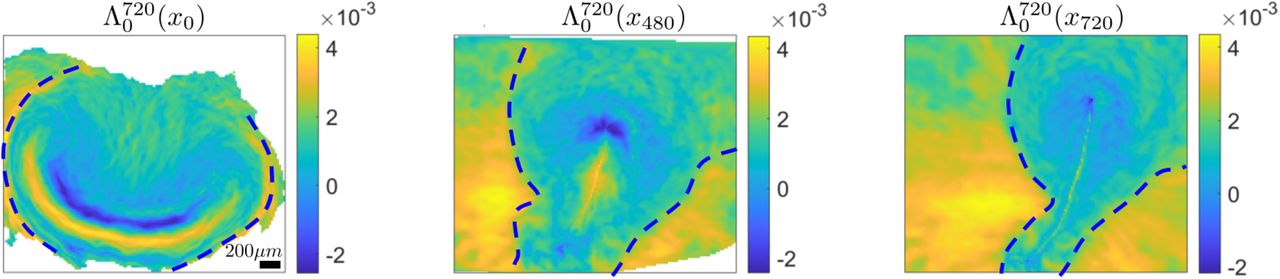
Left) High values of  mark two repellers displayed at x0. The dashed curve marks the EE-EP repeller. Center) Position of the EE-EP repeller after 480min along with the
  visualized on the current cell position
  Right) same as left but after 720min. SM Movie1 shows the corresponding time evolution. Colorbars show attraction rates in min−1.
References
References
- [1].
- [2].
- [3].
- [4].
- [5].
- [6].


