

Summary
A precise estimation of event timing is essential for survival.1 Yet, temporal distortions are ubiquitous in our daily sensory experience.2 A specific type of temporal distortion is the time order error (TOE), which occurs when estimating the duration of events organized in a series.3 TOEs shrink or dilate objective event duration. Understanding the mechanics of subjective time distortions is fundamental since we perceive events in a series, not in isolation. In previous work,4 we showed that TOEs appear when discriminating small duration differences (20 or 60 ms) between two short events (Standard, S and Comparison, C), but only if the interval between events is shorter than 1 second. TOEs have been variously attributed to sensory desensitization,5,6 reduced temporal attention,7,4 poor sensory weighting of C relative to S,8 or idiosyncratic response bias.6
Surprisingly, the serial dynamics of relative event duration were never considered as a factor generating TOEs. In two experiments we tested them by swapping the order of presentation of S and C. Bayesian hierarchical modelling showed that TOEs emerge when the first event in a series is shorter than the second event, independently of event type (S or C), sensory precision or individual response bias. Participants disproportionately expanded first-position shorter events. Significantly fewer errors were made when the first event was objectively longer, confirming the inference of a strong bias in perceiving ordered event durations. Our finding identifies a hitherto unknown duration-dependent encoding inefficiency in human serial perception.
Results
In two separate experiments, we asked human participants to discriminate the duration of a Standard (S) event against that of a Comparison (C) event (or vice versa), and decide which one was longer (two-interval forced choice design, 2IFC). The S event was displayed in first position in Experiment 1, but was shifted to second position in Experiment 2 (Fig 1a). To signal the onset and offset of each event, we used a blue disk as a visual stimulus (see STAR Methods). The interval between cue and first stimulus onset was randomly chosen between 400 and 800 ms. The duration of the S event (120 ms) was kept constant, while the duration of the C event varied, providing participants with three degrees of sensory evidence (weak ±𝛥20; medium ±𝛥60; strong ±𝛥100; Fig 1b). Temporal attention was manipulated by parametrically increasing the Inter-Stimulus Interval (ISI) between S and C (or C and S): 400, 800, 1600, and 2000 ms.

Two-interval forced choice (2IFC) task and model of responses. (a) Timeline of events in the 2IFC task. The Standard stimulus (S) was displayed in the 1st position (experiment 1), and in the 2nd position (experiment 2). We implemented four Inter-stimulus intervals (ISIs) levels: 400, 800, 1600 and 2000 ms. (b) The Standard stimulus had a fixed duration of 120 ms, whereas the durations for the Comparison stimulus varied according to its level of sensory evidence: Weak, Medium, and Strong. (c) Psychometric curves modeling performance on each ISI level of experiments 1 and 2. Points represent data pooled across participants. Lines depict separate fits for each ISI condition, the gray vertical line depict the physical magnitude ϕs of the Standard stimulus, black dots represent the point of subjective equality (PSE) for each ISI condition. The just noticeable difference (JND) is computed from the slopes β of the sigmoid curves. Contrary to experiment 1, all PSEs are shifted to the left side in experiment 2, which exemplifies the time order effect.
We hypothesized that with an ever-changing C in first position (second experiment) the magnitude of time order error (TOE) would increase, as participants would not benefit from orienting attention in time to C in the second position (first experiment). Hence, we expected an interaction between the factors Stimulus presentation order and the orienting of attention in time.9
Sensory precision and temporal distortion profiles
Responses were modeled using individual sigmoid psychometric functions for each ISI level, from which we obtained the midpoint μ and the slope β of each curve (Fig 1c). After fitting the responses, we determined the point of subjective equality (PSE) between S and C, which corresponds to the magnitude μ. We analyzed precision indexed by the just noticeable difference (JND), and the cumulative effect time order errors (TOEs) indexed by the constant error (CE). CE is a global index of temporal distortion. We computed the JND as the β multiplied by the log  ,10,5 and the CE as the difference between the physical magnitude ϕs of the Standard event and μ.
To test changes in the dependent variables as a function of factors ISI and Stimulus presentation order (S first or C first), we quantified the effect of both factors by implementing Bayesian Model Comparison. To do that, we applied a Bayes factor approach to a mixed ANOVA using Bayes’ rule.11,12,13 We built four alternative models: the MISI model (using the ISI as predictor), the ME model (using Experiment as predictor, that is Standard position), the MISI+E (using both factors as predictors), and the MInt model (including ISI and Experiment predictors, but also their interaction). To evaluate the predictive performance of each model, we compared them to the null model M0 (no effect of ISI and Stimulus presentation order) by computing the Bayes factor.9
Just Noticeable Difference (JND)
In experiment 1, the mean JND values were: ISI400 = 29.90 (SD = 15.91), ISI800 = 22.54 (SD = 9.59), ISI1600 = 22.11 (SD = 10.54), and ISI2000 = 20.98 (SD = 11.54). In experiment 2, they were 32.67 (SD = 17.05), 23.97 (SD = 12.01), 25.53 (SD = 14.52), and 26.96 (SD = 14.62), for the ISI400, ISI800, ISI1600 and ISI2000 conditions, respectively (Fig 2a).
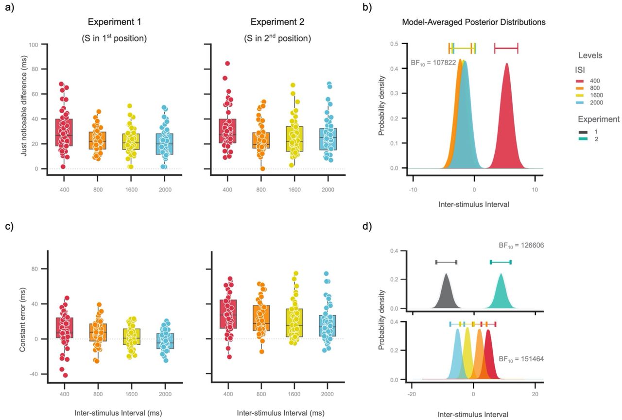
Sensory precision, temporal distortions and model-averaged posterior distributions of the Bayesian models. (a) Just noticeable difference (JND) data plotted as a function of ISI. Box-and- whisker plots show the distribution of the JND. The bottom and top edges indicate the interquartile range (IQR), whereas the median is represented by the horizontal line. The extension of the whiskers is 1.5 times the IQR. Boxplots are overlaid with data of each participant. Results from both experiments seem to follow the same pattern. (b) Bayesian Model Comparison revealed that the JND data were best explained by the MISI model, indicating that, the position of the Standard stimulus does not have modulatory effects on the temporal sensitivity. This result can be visually verified by the clear separation between the distribution ISI400 and the rest of the posterior distributions. (c) Constant errors (CEs) plotted as a function of ISI. We can observe higher and positive CEs values for experiment 2. (d) Distributions of the MISI model signal an effect of ISI, whereas the separated distributions on the ME model reveal an effect of Experiment (i.e., Standard position). Consequently, the Bayes factor revealed that CE data were best modeled by the inferential model including both factors, that is the MISI+E model.
Modeling of the JND data revealed that the data were best explained by the MISI model (BF10 = 107822; see Fig 2b). Post hoc comparisons revealed decisive evidence in favor of statistical differences between the ISI400 and the remaining conditions: ISI800, ISI1600, and ISI2000 (posterior odds = 53596, 284, and 109; respectively). We conclude that Standard position (Experiment factor) does not have modulatory effects on sensory precision, which is driven by temporal attention.
Constant error (CE)
In experiment 1, mean CE values decreased with increasing ISI: ISI400 = 9.18 (SD = 19.32), ISI800 = 7.18 (SD = 14.50), ISI1600 = 1.94 (SD = 12.34), and ISI2000 = -2.60 (SD = 11.30). We found a similar pattern in experiment 2: ISI400 (M = 27.97, SD = 22.82), ISI800 (M = 24.02, SD = 20.12), ISI1600 (M = 20.62, SD = 20.79), and ISI2000 (M = 18.26, SD = 20.78; Fig 2c).
These results were best explained by the MISI+E model (BF10 = 185.6 * 1010). Post hoc comparisons revealed very strong evidence in favor of differences between the ISI400 and the conditions ISI1600 and ISI2000 (posterior odds = 56, 56 and 3189; respectively), but also between the ISI800 and the conditions ISI1600 and ISI2000 conditions (posterior odds = 6 and 118; respectively). The Experiment factor revealed decisive evidence in favor of a statistical difference between experiments 1 and 2 (posterior odds = 4.1 * 1015). That is, increasing ISI helped to minimize CE in both experiments. Participants in experiment 2 made more errors than participants in experiment 1 (Fig 2d).
Relative duration effects
We then analyzed individual discrimination performance at each sensory evidence level (±𝛥100, ±𝛥60, ±𝛥20). We tested how the percentage of accuracy changes as a function of relative duration of the stimuli within a series: “First stimulus longer than the second” and “Second stimulus longer than the first” (Fig 3a,c,e). For each sensory evidence level and duration ordering, we again applied the four Bayesian inferential models (MISI, ME, MISI+E, and MInt) and compared them to the null model M0. These models were carried out after applying an arcsine transformation to the data. This is calculated as two times the arcsine of the square root of the proportion of correct responses.

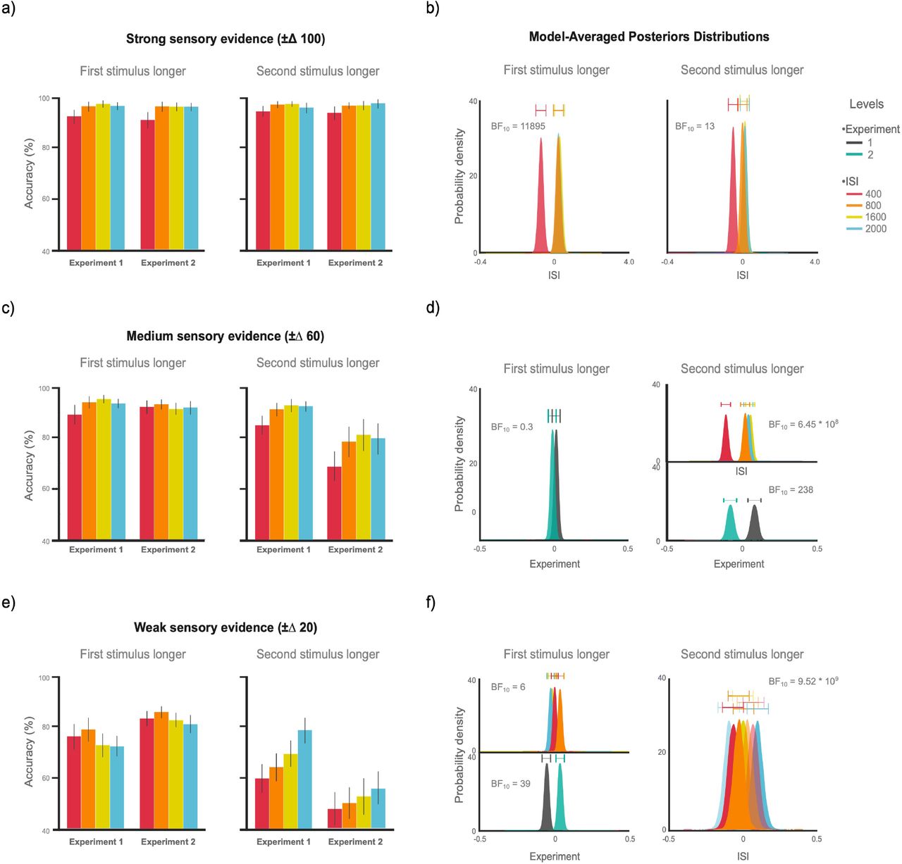
Accuracy and model-averaged posterior distributions of the Bayesian models. a) Strong sensory evidence. Accuracy divided by the position of the longer stimulus, and plotted as a function of ISI and Experiment. Results follow the same pattern independently of the experiment. b) Posterior distributions of the MISI model confirmed that differences between experimental conditions —in the strong sensory evidence — are elicited by the ISI factor. c) For the Medium sensory evidence, when the first stimulus was longer, we found no differences between Experiments or ISI levels. However, the opposite occurred when the second stimulus was longer: we observed a main effect of both factors. d) Posteriors distribution of the medium evidence category: the model ME fails to explain the data for the conditions with first stimulus longer, but for the opposite conditions the data were best modeled by the inferential model including both factors, that is the Model ME+ISI. e) In the Weak sensory category, we observed larger differences in accuracy between experiments and ISI levels. f) Posterior distributions show that for first and second stimulus longer the best models were the ME+ISI and the MInt models, respectively. (Lighter colors signal distributions of the experiment 2).
Strong sensory evidence (±𝛥100)
When the first stimulus was longer, mean accuracy values in experiment 1 were: ISI400 = 92.50, ISI800 = 96.42, ISI1600 = 97.38, and ISI2000 = 96.54. In experiment 2, they were 93.75, 96.59, 96.70, and 97.50, respectively. When the second stimulus was longer, mean accuracy values in experiment 1 were: ISI400 = 94.40, ISI800 = 97.02, ISI1600 = 97.26, and ISI2000 = 95.83. Whereas in experiment 2, they were 90.79, 96.13, 96.02, and 96.02, respectively.
The best model was the MISI model independently of the serial position of the longer stimulus (BF10 = 11895.5; BF10 = 13.5; respectively; Fig 3b). That is, when the sensory evidence for a difference between S and C is strong, behavioral performance is explained solely by the ISI factor, and the relative duration of events in a series is weighted out. When the first stimulus was longer, post hoc comparisons revealed very strong top decisive evidence in favor of a difference between the ISI400 and the remaining conditions (ISI800, ISI1600, and ISI2000, posterior odds = 155, 474, and 88; respectively). Whereas when the second stimulus was longer, we found moderate evidence in favor of a difference between the ISI400 and the long ISI conditions (ISI1600 and ISI2000, posterior odds = 4 and 3; respectively). We found no evidence for a difference between ISI400 and ISI800 (posteriors odds = 1).
Medium sensory evidence (±𝛥60)
When the first stimulus was longer, mean accuracy values in experiment 1 were: ISI400 = 89.28, ISI800 = 94.16, ISI1600 = 95.47, and ISI2000 = 93.69. Whereas in experiment 2, they were 68.75, 78.63, 81.36, and 80.00, respectively. When the second stimulus was longer, mean accuracy values in experiment 1 were: ISI400 = 85.23, ISI800 = 91.54, ISI1600 = 93.09, and ISI2000 = 92.73. In experiment 2, they were 92.27, 93.29, 91.47, and 92.04, respectively.
When the first stimulus was effectively longer, the accuracy data were best explained under the Null model (ME, BF10 = 0.31; MISI, BF10 = 0.15; MInt, BF10 = 0.12; ME+ISI, BF10 = 0.04). When the second stimulus was longer, the ME+ISI was the best model (BF10 = 1.66 * 1011; Fig 3d). Post hoc comparisons of the ISI factor revealed that there was decisive evidence for differences between the ISI400 and the rest of the ISI levels (ISI800, ISI1600, ISI2000, posterior odds = 35985, 2.7 * 106, and 36531; respectively). The Experiment factor revealed too that there is decisive evidence for a difference between experiments 1 and 2 (posterior odds = 2.3 * 107).
Weak sensory evidence (±𝛥20)
When the first stimulus was longer, mean accuracy values in experiment 1 were: ISI400 = 75.83, ISI800 = 78.45, ISI1600 = 72.38, and ISI2000 = 71.90. Whereas in experiment 2, they were 47.5, 49.77, 52.38, and 55.45, respectively. When the second stimulus was longer, mean accuracy values in experiment 1 were: ISI400 = 59.52, ISI800 = 63.92, ISI1600 = 69.04, and ISI2000 = 78.33. In experiment 2, they were 83.06, 85.68, 82.50, and 80.90, respectively.
When first stimulus was longer, the data were best explained by the ME+ISI model (BF10 = 261.9). Post hoc comparisons of the ISI factor revealed moderate evidence for differences between the ISI800 and the ISI levels 16000 and 2000 (posteriors odds = 7 and 10, respectively). We found no differences between the rest of the conditions (all prior odds ≦ 0.3). The Experiment factor revealed decisive evidence for a difference between experiments 1 and 2 (posteriors odds = 35586).
When the longer stimulus was in the second position, the data were best explained by the MInt model (BF10 = 9.5 * 109; Fig 3f). Post-hoc analyses of the ISI factor revealed that there are moderate and decisive evidence for differences between the ISI400 and the conditions ISI1600 and ISI2000 (posteriors odds = 3 and 8824, respectively), but also decisive and moderate evidence for differences between the conditions ISI2000 when compared to the conditions ISI800 and ISI1600 (posteriors odds = 2137 and 10, respectively). The Experiment factor revealed decisive evidence in favor of a difference between experiments 1 and 2 (posteriors odds = 4 * 109).
In experiment 1, post hoc comparisons of the interaction revealed differences between the ISI400 and the conditions ISI1600 and ISI2000 (posteriors odds = 8 and 50889, respectively), but also between the conditions ISI2000 when compared to the conditions ISI800 and ISI1600 (posteriors odds = 1240 and 29, respectively). In Experiment 2, post hoc comparisons revealed that data were best explained under the Null model (all posterior odds ≦ 0.43).
A bias in serial duration perception
We then used a Bayesian hierarchical model to compare differences in the accuracy rate between “First stimulus longer than the second” (ϕa) and “Second stimulus longer than the first” (ϕb) conditions for the uncertain sensory evidence levels ±Δ20 and ± Δ60, which showed an effect of the experimental manipulation (for the Strong sensory evidence, see Supplemental Information). To do that, we applied the Bayesian rate comparison model14 and quantified the difference α between both rates (ϕa and ϕb) as a normally distributed random effect (see STAR Methods; Fig. 4a).

Bayesian rate-comparison model, hypotheses, and prior and posteriors distributions. a) Graphical illustration of the Bayesian rate-comparison model. We tested whether differences α in the accuracy rates ϕa and ϕbare dependent on having the longer stimulus in the first position. To quantify the effect size, we used the parameter δ. b) Our Bayesian model compared the alternative hypothesis H1 (differences in accuracy rate between the conditions “First stimulus longer” and “Second stimulus longer”) versus the null hypothesis H0 (no differences between conditions). Overlapping distributions signal evidence for H0, whereas a shift of the posterior distribution signals evidence in favor of H1. c) For the Medium sensory evidence, we found that posteriors distributions —in experiment 1— yielded evidence in favor of H1 for the short ISIs conditions, but no evidence in the long ISIs. That is, longer waiting times between stimuli lead to a better temporal discrimination. However, this does not occur when the ISI is short, as we can see as we can observe differences in behavioral performance between the conditions “First stimulus longer” longer” and “Second stimulus longer”. d) For experiment 2, all posterior distributions yielded extreme evidence in favor of H1. e-f) We found the same pattern of results for both experiments in the Weak sensory evidence category: In experiment 1, short ISIs (400 and 800 ms) yielded evidence for H1, but we found no evidence in favor in the long ISIs. In experiment 2, all posterior distribution yielded evidence in favor of H1. Overall, these results show that by placing the longer stimulus in the first position, temporal accuracy can be increased.
We applied this model in both experiments for within comparisons at each ISI level. Thus, at each ISI level of each experiment we compared the null hypothesis H0 (no difference in accuracy between ϕa and ϕb rates) versus the alternative hypothesis H1 (Fig. 4b).
Medium sensory evidence (±𝛥60)
Results of experiment 1 yielded strong and moderate evidence in favor of H1 in the conditions ISI400 and ISI800 (BF10 = 12; BF10 = 9; respectively), but no evidence in the longer conditions ISI1600 and ISI2000 (BF10 = 3; BF10 = 0.86; anecdotal evidence in favor of H1 and H0, respectively; Fig 4c). These results confirm that, for short ISIs, participants do more mistakes when the longer stimulus is place in the second position. However, this effect can be minimized by the allocation of attention in time.7,15
Contrary to experiment 1, results of experiment 2 showed decisive evidence for H1 at all ISI levels: ISI400, ISI800, ISI1600 and ISI2000 (BF10 > 10000; BF10 > 10000; BF10 = 310; BF10 = 1512; respectively; Fig 4d). That is, when sensory evidence is of medium strength, temporal attentions does not help to minimize temporal errors. Regardless of the ISI, participants do more mistakes when the longer stimulus is placed in the second position.
Weak sensory evidence (±𝛥20)
We found similar results in the weak sensory evidence. In experiment 1, results yielded extreme evidence in favor of H1 in the conditions ISI400 and ISI800 (BF10 = 2945; BF10 = 3013; respectively), but no differences in the longer ISIs: 1600 and 2000 (BF10 = 0.59; BF10 = 2; respectively; Fig. 4e). In experiment 2, results showed extreme evidence for H1 at each ISI level (BF10 > 10000; BF10 > 10000 ; BF10 > 10000; BF10 > 10000; respectively; Fig. 4f).
Response bias
Finally, we tested whether participants were biased in hitting the keys for “S” or “C”. We abstracted away from the confounding factor of sensory uncertainty by analyzing key responses across ISI levels at the Strong sensory evidence level only (±𝛥100). We applied individual Bayesian binomial analyses to the set of responses, and verifed the null hypothesis H0 of a 50% probability to choose either S or
C. In both experiments, results yielded Bayes factors (BF01) with moderate evidence in favor of the null hypothesis (Supplemental InformationFig 2). For experiment 1, the lower and higher values for the BF were 4.5 and 10.1, respectively. Whereas for experiment 2, they were 3.6 and 10.1. Overall, button press data were between 3.6 and 10.1 more likely under the null hypothesis (no bias) than under the alternative hypothesis, discarding the presence of an idiosyncratic response bias in some of the participants.
Discussion
Time order error (TOE) is a subjective distortion of an event’s duration that occurs when the event is inserted in a series. It constitutes one of the oldest and least understood phenomena of subjective time perception.16,17,18 A set of models have been proposed to try and explain how TOEs are generated. In the sensation-weighting model,8 temporal distortions would arise because the sensory effects produced by S and C are differentially weighted before they are discriminated. In the difference model,6 TOEs depend on two components: 1) Desensitization caused by short inter-stimulus intervals (ISIs) —akin to a form of attentional blink19— not allowing the sensory system to reset back to its initial state;5 2) an idiosyncratic response bias in picking a specific stimulus (always picking the first, or the second one). Both models predict that by improving stimulus encoding processes, such as by increasing ISI and thus temporal attention to the second stimulus in a series, TOE should decrease. We verified this stance in our previous work4 using a visual two-interval forced-choice (2IFC) task with empty events in a fixed order, with the comparison (C) event always following the standard (S) event. However, all accounts missed the crucial point of explaining how TOEs are generated under uncertain sensory evidence and limited attention resources.
Although a meta-analysis21 suggested that temporal sensitivity decreases when the Standard event is displayed in the 2nd position, our results demonstrate no effect of S position on temporal sensitivity, which was modulated only by the ISI factor. We conclude that TOEs are not elicited by differences in sensory precision. Our analysis of key presses shows that participants were not biased in hitting the key for “S” or “C”. That is, TOEs are not generated by an absolute positional bias, as predicted by the difference model.6
Since TOEs occur during serial discrimination tasks, we tested whether event duration dynamics is the primary source of distortions by flipping the positions of standard (S) and comparison (C) events in two separate behavioral experiments. First, we replicated the finding that increasing the temporal interval between first and second event minimizes TOEs for S in both 1st and 2nd position, although significantly less frequently for S in 2nd position. These results can be explained by the beneficial effects of allocating attention in time, more oriented to the encoding unpredictable events (C).7,20,15
Second, a Bayesian modelling of accuracy at each sensory level (𝛥100, 𝛥60, 20𝛥) showed that, while most TOEs occur for short ISIs and small to medium sensory evidence, they tend to cluster in a specific serial condition: When the first stimulus in a series is shorter than the second stimulus, regardless of whether it is S or C. In such a case, participants were biased to say that the first event was longer, consistently making mistakes.
When the first stimulus was truly larger than the second, performance was significantly above chance, suggesting optimal processing even under uncertain sensory circumstances (small and medium sensory evidence, 20/60 ms). This prefigures a novel order bias in serial perception based on duration-dependent relative positions of stimuli, which can only be partially counteracted by increasing temporal attention. Attention helps when S is in the first position, as it enhances the encoding of the C stimulus whose duration is unpredictable.
Our new model finally explains that time order errors arise under sensory uncertainty because of serial perceptual encoding inefficiency. Future research is needed to uncover the physiological basis of such a strong expectation about the temporal statistics of incoming stimuli.
STAR Methods
Participants
Experiment 1
Part of the results for experiment 1 were previously published.4 This dataset has a sample of 52 participants (34 female; ages: 18-33; mean age: 24.42). We removed participants with an accuracy ≤ 55 %, as this is an indicator that they completed the task by chance. One participant was removed due to his low accuracy. For each participant we computed the goodness-of-fit of the psychometric function (R2). Participants with a R2 value lower than two standard deviations away from the mean were removed. Seven participants were removed from analysis following this procedure. For the dependent variables WF and CE, we also discarded extreme outliers. We identified these outliers by using two standard deviations. Two participants were discarded for being marked as extreme outlier in experiment 1. Therefore, the final sample included the data from 42 participants (26 female; ages: 18-33; mean: 24.14).
Experiment 2
We had an initial sample of 58 participants in experiment 2 (45 female; ages: 18-37; mean age: 25.41). We applied the same procedure as in experiment 1 for discarding outliers. Four participants were removed from analysis due to their low performance of correct responses (< 55%). Nine participants were removed from analysis due to their low R2 values. One participant was discarded for being marked as extreme outliers in the WF. Therefore, the final analysis included the data from 44 participants (34 female; ages: 18-32; mean: 25.22). In total, we report on the behavior of 86 participants.
Individuals were recruited through online advertisements. Participants self-reported normal or corrected vision and had no history of neurological disorders. Up to three participants were tested simultaneously at computer workstations with identical configurations. They received 10 euros per hour for their participation. The studies were approved by the Ethics Committee of the Max Planck Society. Written informed consent was obtained from all participants previous to the experiment.
Design
We used a classical interval discrimination task by using a 2IFC design, where participants were presented with two visual durations: S and C.22,23 S had a magnitude of 120 ms and was always displayed in the first position in experiment 1, but in the second position in experiment 2. In both experiments, we used three magnitudes for the step comparisons 𝛥 between S and C: 20, 60, and 100 ms. We derived the magnitudes for the C stimuli as S ± 𝛥, which resulted in the next C durations: 20, 60, 100, 140, 180, and 220 ms. For the ISI, we used four durations: 400, 800, 1600, and 2000 ms. For each trial, the inter-trial interval (ITI) was randomly chosen from a uniform distribution between 1 and 3 seconds. Participants judged whether the S or C interval was the longer duration, and responded by pressing one of two buttons on an RB-740 Cedrus Response Pad (cedrus.com, response time jitter < 1 ms, measured with an oscilloscope).
Stimuli and Apparatus
We used empty visual stimuli, which were determined as a succession of two blue disks with a diameter of 1.5° presented on a gray screen.24 We used empty stimuli to ensure that participants were focused on the temporal properties of the stimuli.25 All stimuli were created in MATLAB R2018b (mathworks.com), using the Psychophysics Toolbox extensions.26,27,28 Stimuli were displayed on an ASUS monitor (model: VG248QE; resolution: 1,920 × 1,080; refresh rate: 144 Hz; size: 24 in) at a viewing distance of 60 cm.
Protocol (Task)
The experiment was run in a single session of 70 minutes. Participants completed a practice set of four blocks (18 trials in each block). All sessions consisted of the presentation of one block for each ISI condition. Each block was composed of 120 trials and presented in random order. In order to avoid fatigue, participants always had a break after 60 trials. Each trial began with a black fixation cross (diameter: 0.1°) displayed in the center of a gray screen. Its duration was randomly selected from a distribution between 400 and 800 ms. After a blank interval of 500 ms, S was displayed and followed by C, after one of the ISI durations.
Participants were instructed to compare the durations of the two stimuli by pressing the key “left”, if S was perceived to have lasted longer, and the key “right” if C was perceived to have lasted longer. After responding, they were provided with immediate feedback: the fixation cross color changed to green when the response was correct, and to red when the response was incorrect.
Data analysis
The data analysis was implemented with Python 3.7 (python.org) using the ecosystem SciPy (scipy.org) and the libraries Pandas,29 Seaborn,30 and Pingouin.31 Frequentist statistical analyses were executed in Pingouin. Bayesian statistical analyses were implemented using the BayesFactor package for R.9 All data and statistical analyses were performed in Jupyter Lab (jupyter.org).
To endorse open science practices and transparency on statistical analyses, we used JASP32 (jasp-stats.org) for providing statistical results (data, plots, distributions, tables and post hoc analyses) of both Frequentist and Bayesian analyses in a graphical user-friendly interface. These results can be consulted at Open Science Framework as annotated .jasp files (osf.io/jkzq4/). As JASP uses the BayesFactor package as a backend engine, the default prior distributions of this package were the same for JASP. Modelling of the Bayesian rate-comparison model14 was done in MATLAB R2018b (mathworks.com) using JAGS 4.3.033 (www.mcmc-jags.sourceforge.net/).
Psychometric curves
Responses were modeled using a 6-point psychometric function using the nonlinear least-squares fit in Python. We plotted the six C durations on the x -axis and the probability of responding “C longer than S” on the y -axis. We parameterized psychometric functions by using the distribution of a logistic function f, which is given by
 where L is the maximum value of f, x is the magnitude of the C stimuli, μ is the x-value at the mid-point of the psychometric function, and β parametrizes the slope of the logistic function. Two indices of temporal performance are extracted from this fitting: a marker for the perceived event duration, and a marker for the sensory temporal precision.34 The perceived duration was measured via the PSE (μ in equation 1), i.e., the value on the x-axis that corresponds to the 50% value on the y-axis.34 We derived the CE from the PSE, which is defined as the difference between the PSE and the magnitude of the physical duration ϕs of S:
 Positive CEs indicate that the C stimuli were perceived as shorter than the S stimulus. The temporal sensitivity was measured by using the JND, which is defined as being half the interquartile range of the fitted function
  , where x . and x .25 denote the point values on the y -axis that output 25% and 75% “longer” responses. The smaller the JND, the higher the discrimination sensitivity of the sensory system. The JND is obtained from the slope (β in equation 1) of the fitted function:

Statistical analyses
Frequentist analyses
Frequentist statistical analyses are available at Open Science Framework (osf.io/jkzq4/). For the Frequentist analyses the level of statistical significance to reject the null hypothesis H0 was set to α = 0.05. To test for significant changes in the dependent variables, we implemented a repeated measures ANOVA across ISI levels in both experiments. We carried out post hoc comparisons by using the Bonferroni correction  .
.
Bayesian Model Comparison
To contrast results from both experiments, we applied a Bayes Factor approach to ANOVA by using Bayesian Model Comparison (BMC).13,35 Tod do that, we implemented Bayes’ rule for obtaining the posterior distribution p(θ ∣ D), where D expresses the observed data, under the model specification M1,11,14 which is given by
 where p(D ∣ θ, M1) denotes the likelihood, p = (θ ∣ M1) expresses the prior distribution, and the marginal likelihood is expressed by p(D ∣ M1). Bayes factor ANOVA compares the predictive performance of competing models. Thus, for evaluating the relative probability of the data D under competing models we computed the Bayes factor (BF): Let BF10 express the Bayes factor between a null model M0 versus an alternative model M1. The predictive performance of these models is given by the probability ratio obtained by dividing the marginal likelihoods of M1 and M0:
 In this case, BF10 expresses to which extent the data support the model M1 over M0, whereas BF01 indicates the Bayes factor in favor M0 over M1. BF values < 0 give support to M0, whereas BF > 1 support the M1 model. A BF of 1 reveals that both models predicted the data equally well.36 For our analysis of the dependent variables we build four alternative models (ME, MISI, MISI+E, and the MInt) for quantifying the effect of two factors: ISI and Standard position. The ME model uses the Standard position as predictor, whereas the MISI model uses the ISI. The MISI+E model uses both factors as predictors (the ISI and the Standard position), and the MInt model uses again both factors but includes also their interaction (ISI * Experiment). The prior model probability p(M) of each model was set to be equal, i.e., prior model odds of 0.2. We compare each model to the null model M0 and provided the BF. The model with the highest BF was selected as the best model, and thus is the inferential model that explain the data more accurately.
Bayesian post hoc testing is based on pairwise comparisons using Bayesian t-tests with a Cauchy  prior. For post hoc testing, the posterior odds are corrected for multiple testing by fixing to 0.5 the prior probability that the null hypothesis holds across comparisons.36 For all our analyses we used the default prior values for Bayes factor ANOVA,37,38 which are also the default values in the BayesFactor package and JASP.
Bayesian rate-comparison model
To test individual differences on the accuracy-rate θ between the conditions a (“First stimulus longer”) and b (“Second stimulus longer”), we used the Bayesian comparison-rate model (see Fig. 4a) for computing differences between θa and θb.14 We deployed the Bayesian comparison-rate model for within subject comparisons at each ISI level and modeled differences between conditions as having Gaussian distributions. That is, with mean μ and standard deviation σ:
 This model receives two inputs for each subject i: the number of trials n and the total number of correct responses s. We assumed that the rate parameter θ follows a binomial distribution. In order to model θ as a normally distributed variable, we applied a probit transformation, which transforms θ (a real number) into a probability ϕ:39
 We added a variable δ to quantify the strength of the effect size:
 Then, we modeled the effect α as random effect. That is, with a Gaussian distribution of mean μα and standard deviation σα:
 Thus, differences between conditions are given by adding the effect α to one of the transformed rates ϕ:
 To run this model, we generated 50 chains with 100000 samples, which generated a total of 5000000 samples. We discarded the first 1000 burn-in samples. Posterior distributions of this model show visually the strength of the effect size δ. We computed the Bayes factors for this model using the Savage-Dickey method.40,14
Author contributions
Research question: FS and AT. Study design: All authors. Testing and data collection: FS. Data analysis and writing original draft: FS and AT. Writing, review & editing: all authors.
Declaration of interests
The authors declare no competing interests.
Supplemental information
Strong sensory evidence (±𝛥100). Results of experiment 1 yielded anecdotal evidence in favor of H0 in all conditions: ISI400, ISI800, ISI1600 and ISI2000 (BF10 = 0.29; BF10 = 0.51; BF10 = 0.81, BF10 = 0.94; respectively; Fig SI 1a). We found similar results in experiment 2 for the conditions ISI400, ISI800, ISI1600 and ISI2000 (BF10 = 0.38; BF10 = 0,58; BF10 = 0.52; BF10 = 0.34; respectively; Fig SI 1b). That is, when sensory evidence for C is strong, no duration-dependent bias can be detected.

Strong sensory evidence category and posteriors distributions of the Bayesian rate-comparison model. a) Results yielded that when the Standard duration is in the first position (Experiment 1), at each ISI level there is no evidence for H1. Thus, no differences between the conditions “First stimulus longer” and “Second stimulus longer” can be claimed. This can be visually verified by the overlapping distributions at each ISI level. b) The same was true when the Standard event was displayed in the second position (Experiment 2): The Bayes factor showed no evidence for H1, but anecdotal evidence for H0. Thus, when there is a strong sensory difference between stimuli, no differences in accuracy rate between the conditions “Long stimulus first” and “Long stimulus second” can be claimed.

Results of the Bayesian Binomial analyses of the Strong sensory evidence condition. Bayes factors (BF10) revealed that there is no individual bias in responses either in experiment 1 or experiment 2. Results yielded evidence in favor of the null hypothesis (no differences between responses “First stimulus longer” or “Second stimulus longer”).
Acknowledgements
We thank Lauren Fink and Luigi Acerbi for critical suggestions.


