

ABSTRACT
Our ability to remember the past is essential for guiding our future behavior. Psychological and neurobiological features of declarative memories are known to transform over time in a process known as systems consolidation. While many theories have sought to explain the time-varying role of hippocampal and neocortical brain areas, the computational principles that govern these transformations remain unclear. Here we propose a theory of systems consolidation in which hippocampal-cortical interactions serve to optimize generalizations that guide future adaptive behavior. We use mathematical analysis of neural network models to characterize fundamental performance tradeoffs in systems consolidation, revealing that memory components should be organized according to their predictability. The theory shows that multiple interacting memory systems can outperform just one, normatively unifying diverse experimental observations and making novel experimental predictions. Our results suggest that the psychological taxonomy and neurobiological organization of declarative memories reflect a system optimized for behaving well in an uncertain future.
INTRODUCTION
Memory, the process by which experience is stored and transformed in neural circuits, lies at the heart of our ability to make adaptive decisions1. It is threaded through cognition, from perception through spatial navigation to decision-making and explicit conscious recall. Befitting the central importance of memory, brain regions including the hippocampus appear specifically dedicated to this challenge2–4.
The concept of memory has refracted through psychology and neurobiology into diverse subtypes and forms that have been difficult to reconcile. Taxonomies of memory have been drawn on the basis of psychological content, for instance differences between memories for detailed episodes and semantic facts5; on the basis of anatomy, for instance differences between memories that are strikingly dependent on hippocampus versus those that are not6; and on the basis of computational properties, for instance differences between memories reliant on pattern-separated or distributed neural representation7. Many previous theories have tried to align and unify psychological, neurobiological, and computational memory taxonomies8–12. However, none yet resolve long-standing debates on where different kinds of memories are stored in the brain, and, fundamentally, why different kinds of explicit memories exist.
Classical views of systems consolidation, such as the standard theory of systems consolidation8,13,14, have held that memories reside in hippocampus before transferring completely to neocortex (Fig. 1a). Related neural network models, such as the complementary learning systems theory, have further offered a computational rationale for systems consolidation based on the benefits of coupling complementary fast and slow learning systems9,15. However, these theories lack explanations for why some memories remain forever hippocampal dependent, as shown in a growing number of experiments16,17. On the other hand, more recent theories, like multiple trace theory11,18 and trace transformation theory19,20, hold that the amount of consolidation can depend on memory content, but they do not provide a quantitatively clear criterion for what content will consolidate, nor why this might be beneficial to behavior.

(a) The standard theory of systems consolidation. (b, c) Our theoretical framework assumes that neocortex extracts and encodes environmental relationships within the weights between distributed neocortical neurons in a process mediated by hippocampal reactivations. (d) Cartoon of the teacher-student-notebook formalism; subscripts “i” and “o” refer to input and output layers. (e) Core neural network model architecture (see Methods for details). (f-k) Stages of learning and inferences in the model.
One possible way forward is to see that memories serve not only as veridical records of experience, but also to support generalization in novel circumstances21–26. Here we introduce a mathematical neural network theory of systems consolidation founded on the principle that memory systems and their interactions collectively optimize generalization. The resulting theory unifies diverse experimental phenomena that have vexed prior theories, explains why multiple interacting brain areas are beneficial, and reveals that the predictability of experiences should determine when and where memories reside. Our results provide a quantitative and unified picture of the organization of explicit memories based on their utility for future adaptive behavior.
RESULTS
Formalizing systems consolidation
We conceptualize an animal’s experiences in the environment as structured neuronal activity patterns that the hippocampus rapidly encodes and the neocortex gradually learns to produce internally9,15,27,28 (Fig. 1b). We hypothesize that systems consolidation allows neocortical circuits to learn many structured relationships between different subsets of these active neurons. Focusing on one of these relationships at a time, neocortical circuitry might learn to produce the responses of a particular output neuron from the responses of other input neurons (Fig. 1c). For example, in a human, an output neuron contributing to a representation of the word “bird” might receive strong inputs from neurons associated with wings and flight. In a mouse, an output neuron associated with freezing might receive strong inputs from neurons associated with the sound of an owl, the smell of a snake, or the features of a laboratory cage where it had been shocked29.
We first sought to develop a theoretically rigorous mathematical framework to formalize this view of how systems consolidation contributes to learning. Our framework builds on the complementary learning systems hypothesis9,15, which posits that fast learning in hippocampus guides slow learning in neocortex to provide an integrated learning system that outperforms either subsystem on its own. Here we formalize this notion as a neocortical “student” that learns to predict an environmental “teacher,” aided by past experiences recorded in a hippocampal “notebook” (Fig. 1d). We note that other anatomical mappings may be possible30–32.
We modeled each of these theoretical elements with a simple neural network that permitted analytical analysis (Fig. 1e, Methods). Specifically, we modeled the teacher as a linear feedforward network that generates input-output pairs through fixed weights with additive output noise, the student as a size-matched linear feedforward network with learnable weights33–35, and the notebook as a sparse Hopfield network36–38. The student learns its weights from a finite set of examples (experiences) that contain both signal and noise. We modeled the standard theory of systems consolidation by optimizing weights for memory. This means that the squared difference between the teacher’s output and the student’s prediction should be as small as possible, averaged across the set of past experiences. Alternatively, we hypothesize that a major goal of the neocortex is to optimize generalization. This means that the squared difference between the teacher’s output and the student’s prediction should be as small as possible, averaged across possible future experiences that could be generated by the teacher.
Learning starts when the teacher activates student neurons (Fig. 1f, gray arrows). The notebook encodes this student activity by associating it with a random pattern of sparse notebook activity using Hebbian plasticity (Methods; Fig. 1f, pink arrows). This effectively models hippocampal activity as a pattern-separated code for indexing memories39,40. The dynamics of the notebook’s recurrent notebook network implement pattern completion36,41, whereby full notebook indices can be reactivated randomly from spontaneous activity or purposefully from partial cues42 (Methods; Fig. 1g). Student-to-notebook connections allow the student to provide the partial cues that drive pattern completion (Fig. 1g, orange arrows). Notebook-to-student connections then allow the completed notebook index to reactivate whatever student representations were active during encoding (Fig. 1g, blue arrows). Taken together, these three processes permit the student to use the notebook to recall memories from related experiences in the environment. Thus, our theory concretely models how the neocortex could use the hippocampus for memory recall.
We model systems consolidation as plasticity of the student’s internal synapses (Figs. 1h, 1i). The student’s plasticity mechanism is guided by notebook reactivations (Fig. 1h), similar to how hippocampal replay is hypothesized to contribute to systems consolidation43. Slow, error-corrective learning aids generalization44, and here we adjust internal student weights with gradient-descent learning (Fig. 1i). Specifically, we assume that offline notebook reactivations provide targets for student learning (Methods), where the notebook-reactivated student output is compared with student’s internal prediction to calculate an error signal for learning. We consider models that set the number of notebook reactivations to optimize either memory transfer or generalization. Furthermore, the system can use the notebook (Fig. 1j) or only the learned internal student weights (Fig. 1k) to make output predictions from any input generated by the teacher. Our model uses whichever pathway makes statistically better predictions.
Generalization-optimized complementary learning systems (Go-CLS)
We next simulated the dynamics of memorization and generalization in the teacher-student-notebook framework to investigate the impact of systems consolidation. We first modeled the standard theory of systems consolidation as limitless notebook reactivations that optimized student memory recall (Fig. 2a, c, e, Methods). Learning begins when the notebook stores a small batch of examples, which are then repetitively reactivated by the notebook in each epoch to drive student learning (Methods). In separate simulations, examples were generated by one of three teachers that differed in their degree of predictability, here controlled by the signal-to-noise ratio (SNR) of the teacher network’s output (Fig. 1e, Methods). The notebook was able to accurately recall the examples provided by each teacher from the beginning (Fig. 2a, c, e, dashed blue lines), and we showed mathematically that recall accuracy scaled with the size of the notebook (Supplementary Material 5.2). Notebook-mediated generalization (Student In → Notebook → Student Out) was poor for all three teachers (Fig. 2a, c, e, dashed red lines), as rote memorization poorly predicts high-dimensional stimuli that were not previously presented or memorized (Supplementary Material 5.3). The student gradually reproduced past examples accurately (Fig. 2a, c, e, solid blue lines), but the signal in each example was contaminated by whatever noise was present during encoding and repetitively replayed throughout learning. Therefore, although the generalization error decreased monotonically for the noiseless teacher (Fig. 2a, solid red line), noisy teachers resulted in the student eventually generalizing poorly (Fig. 2c, e, solid red lines). From a mathematical point of view, this is expected, as the phenomenon of overfitting to noisy data are well appreciated in statistics and machine learning45,46.

(a-h) Dynamics of student generalization error, student memorization error, notebook generalization error, and notebook memorization error when optimizing for student memorization (a, c, e, g) or generalization (b, d, f, h) performance. The student’s input dimension N = 100, and the number of patterns stored in the notebook P = 100 (all encoded at epoch = 1; epochs in the x-axis correspond to the time passage during systems consolidation). Notebook contains M = 2000 units, with a sparsity a = 0.05. During each epoch, 100 patterns are randomly sampled from the P stored patterns for reactivation and training the student. The student’s learning rate is 0.015. Teachers differed in their levels of predictability (a, b: SNR = infinity; c, d: SNR = 4; e, f: SNR = 0.05; g, h: SNR ranges from 2-4 to 24). (i-l) Memorization and generalization scores for the integrated student-notebook system as a function of time and SNR, when optimized for student memorization (i, k) or generalization (j, l). Memory and generalization scores are translated from respective error values by Score = (E0 −Et)/E0, E0 and Et are the generalization or memory errors before training starts and at epoch = t, respectively. Effect of notebook lesion on memory performance (cyan and orange lines, orange lines are simply the two-point version of the cyan lines) depended on optimization objective and time (i, j).
The implications of these findings for psychology and neuroscience are far reaching, as the standard theory of systems consolidation assumes that generalization follows naturally from hippocampal memorization and replay; it does not consider when systems consolidation is detrimental to generalization. For example, previous neural network models of complementary learning systems focused on learning scenarios where the mapping from input to output was fully reliable8,9. A goose is always a bird, and a rose is always a flower. Within our teacher-student-notebook framework, this means that the teacher is noiseless and perfectly predictable by the student architecture. In such scenarios, standard systems consolidation continually improved both memorization and generalization in our model (Fig. 2a, solid red line). However, for less predictable environments, our theory suggests that too much systems consolidation can severely degrade generalization performance by leading the neocortex to overfit to unpredictable elements of the environment (Fig. 2c, solid red). In highly unpredictable environments, any systems consolidation at all can be detrimental to generalization (Fig. 2e, solid red). If the goal of systems consolidation is full memory transfer, then our theory illustrates that the system pays a price in reduced ability to generalize in uncertain environments.
Given the intricate effect of training example replay on generalization, what systems consolidation strategy would optimize generalization? Here we propose generalization-optimized complementary learning systems (Go-CLS) theory, which considers the normative hypothesis that the amount of systems consolidation is adaptively regulated to optimize the student’s generalization accuracy based on the predictability of the input-output mapping (Fig. 2b, d, f). For the teacher with high degree of predictability, the student’s generalization error always decreased with more systems consolidation (Fig. 2b, solid red line), and the student could eventually recall all stored memories (Fig. 2b, solid blue line). Memory transfer therefore arises as a property of a student that learns to generalize well from this teacher’s examples. In contrast, a finite amount of consolidation (here modeled by a fixed number of notebook reactivations) was necessary to minimize the generalization error when the teacher had limited predictability (Fig. 2d, f), and our normative hypothesis is that systems consolidation halts at the point where further consolidation harms generalization (Fig. 2d, f, vertical black dashed line). The resulting student could generalize near optimally from each of the teachers’ examples (Fig. 2d, f, solid red lines, Supplementary Material 7.2), but its memory performance was hurt by incomplete memorization of the training data (Fig. 2d, f, solid blue lines). Nevertheless, the notebook could still recall the memorized examples (Fig. 2b, d, f, dashed blue lines). Go-CLS thus results in an integrated system that can both generalize and memorize by using two systems with complementary properties. We note that implementing this strategy for regulated systems consolidation requires a supervisory process capable of estimating the predictability of experience and the optimal amount of consolidation, a topic we address in the Discussion.
These examples show that the dynamics of systems consolidation models interestingly depend on the degree of predictability of the teacher. We therefore leveraged our analytical results to comprehensively compare the standard theory of systems consolidation to the Go-CLS theory for regulated systems consolidation for all degrees of predictability (Supplementary Material 6, 7). Standard systems consolidation eventually consolidated all memories for any teacher (Fig. 2g, blue). As anticipated by Fig. 2a-f, the generalization performance varied dramatically with the teacher’s degree of predictability (Fig. 2g, red). Generalization errors were higher for less predictable teachers, and optimal consolidation amounts were lower. Therefore, regulated systems consolidation removed the detrimental effects of overfitting (Fig. 2h, red) but ended before the student could achieve perfect memorization (Fig. 2h, blue, non-zero error). Both the generalization performance and the memory performance improved as the teacher’s degree of predictability increased (Fig. 2h).
The experimental literature on the time course of systems consolidation and time-dependent generalization provides important constraints on our theory. We thus sought to model these effects by translating mean square errors (Fig. 2 g, h) into memory retrieval scores, where 0 indicates random performance and 1 indicates perfect performance (Fig. 2i-l, Methods). Our framework can use either the student or the notebook to recall memories or generalize (Fig. 1j, k), and we model the combined system by making predictions with whichever subsystem is more accurate (Methods). We simulated hippocampus lesions by disallowing the combined system from using notebook outputs and ending systems consolidation at the time of the lesion (Fig. 2i, j, cyan). Note that the combined memory (Figs. 2i, j) and generalization scores (Figs. 2k, l) often map onto the notebook and student performances, respectively, but it is also possible for the better subsystem to switch over time (Supplemental Material 6.1). As it takes time for the student to learn accurate generalizations, our systems consolidation models exhibit time-dependent generalization (Fig. 2k, l, purple). In contrast, the notebook permitted accurate memory retrieval from the start (Fig. 2i, j, black).
Standard systems consolidation and regulated systems consolidation make strikingly different predictions for how retrograde amnesia and time-dependent generalization curves depend on the teacher’s degree of predictability (Fig. 2i-l). As expected, notebook lesions always produced temporally graded retrograde amnesia curves in the standard theory13 (Fig. 2i, orange). When systems consolidation was instead optimized for generalization, the effects of notebook lesions depended strongly on the predictability of the teacher (Fig. 2j, orange). In particular, the model could produce both graded and flat retrograde amnesia curves, with the slope of the amnesia curve increasing with the degree of predictability. Diverse generalization curves resulted from either model of systems consolidation (Fig. 2k, l), with maximal generalization performance increasing with the predictability of the teacher. However, student overfitting meant that only regulated systems consolidation maintained this performance over time. Standard systems consolidation could even result in a student that generalized maladaptively, resulting in worse-than-chance performance where the trained student interpolates noise in past examples to produce wildly inaccurate outputs (Fig. 2k).
Go-CLS explains diverse experimental results
These results allow Go-CLS theory to explain diverse experimental findings. Since real world experiences are composed of many elements that differ in their degree of predictability, our theory predicts that different components of human memory will consolidate to different degrees. In human memory research, patients with selective hippocampal damage indeed show retrograde amnesia reflecting diverse dynamics of systems consolidation17,47. Researchers usually classify hippocampal amnesia dynamics according to whether memory deficits are similar for recent and remote memories (flat retrograde amnesia), more pronounced for recent memories (graded retrograde amnesia), or absent for both recent and remote memories (no retrograde amnesia) (Fig. 3a). Some patients show graded retrograde amnesia consistent with the standard theory, while others either have flat retrograde amnesia or no retrograde amnesia17 (Fig. 3b). Regulated systems consolidation can recapitulate this diversity of retrograde amnesia curves (Fig. 3c). High and low predictability experiences lead to graded and flat retrograde amnesia, respectively (Figs. 2j, 3c, solid lines). A period of prior consolidation of highly predictable experiences decreases the slope of graded retrograde amnesia (Fig. 3c, dashed light-blue lines), and it’s possible to see no retrograde amnesia at all when the prior consolidation was extensive (Fig. 3c, dashed orange line, Methods). This conceptually resembles schema-consistent learning48. Similarly diverse retrograde amnesia curves have been seen in rodent memory tasks (Figs. 3d-g). For example, hippocampal lesions can result in either graded or flat retrograde amnesia in different individuals performing the same task49–51 (Figs. 3d-f), and individual animals can exhibit different types of amnesia on different tasks51. (Figs. 3f, g). In summary, our theory accounts parsimoniously for this wide range of experimental observations through the tuning of two parameters: the predictability of experience and the amount of prior consolidation.
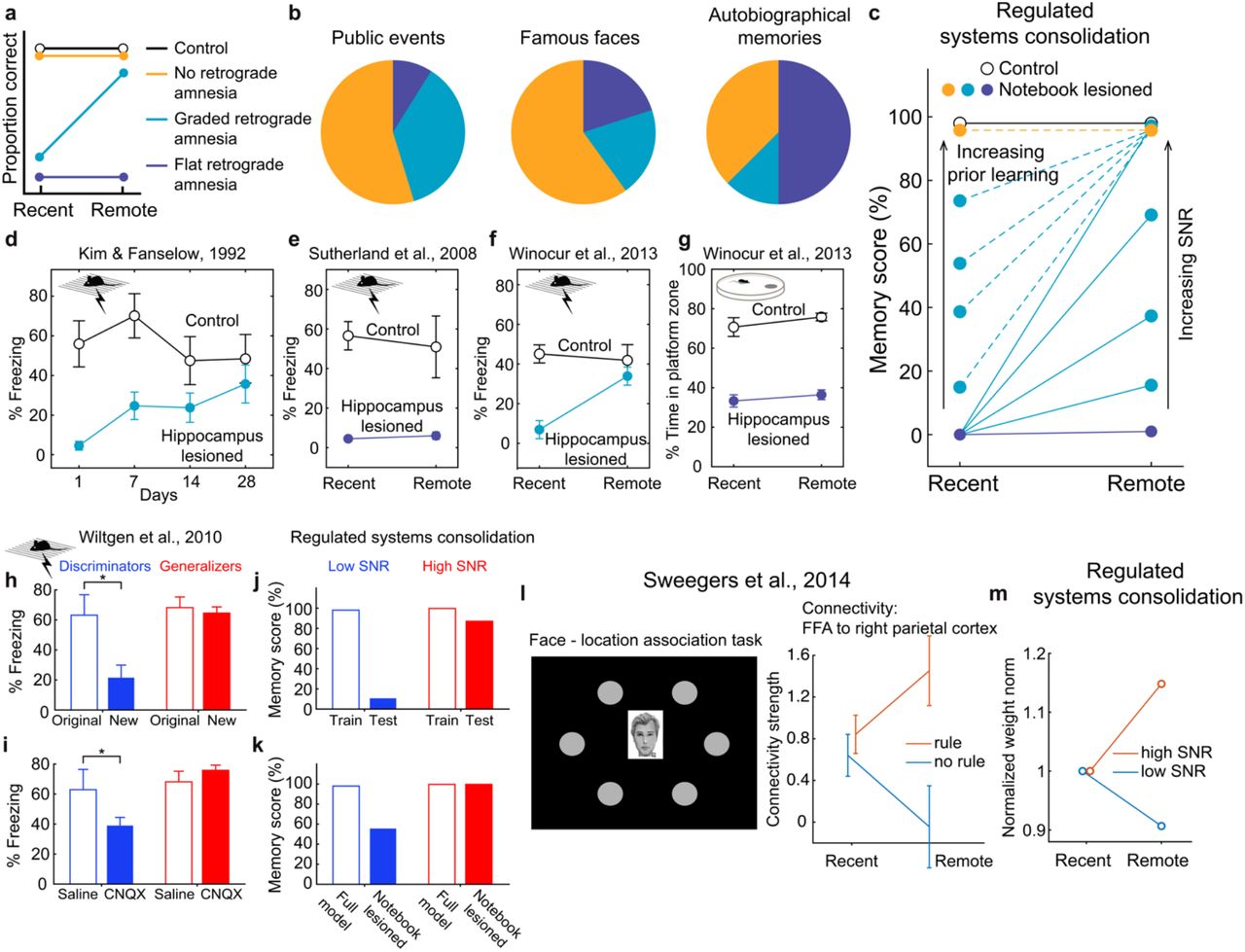
(a) Schematic of retrograde amnesia curves. (b) Reports of retrograde amnesia in human patients with selective hippocampal damage show diverse dynamics. Figure adapted from Yonelinas et al., 201917. (c) Regulated systems consolidation can reproduce the diversity of retrograde amnesia curves (see Methods for model details). (d, e) Lesioning hippocampus in rodents can produce both graded and flat retrograde amnesia. Figure adapted from Kim & Fanselow, 199257, Sutherland et al., 200850. Lesioning the hippocampus can result in graded (f) or flat (g) retrograde amnesia in the same animal performing different tasks (contextual fear conditioning and Morris water maze, respectively). Figure adapted from Winocur et al., 201351. (h) Discriminators can differentiate the original fear-conditioning context with another similar but novel context, whereas generalizers show similar amount of fear response to both contexts. (i) Silencing the hippocampus in mice 15 days after contextual fear conditioning differentially impact fear memory of the original context, depending on whether the animal show time-dependent fear generalization. panels h and i are adapted from Wiltgen et al., 201058. (j, k) Regulated systems consolidation can reproduce similar correlation between time-dependent generalization and reduced hippocampal dependence of memories. High SNR (1000) and low SNR (0.6) simulations based on analytical solutions are used to model the “generalizers” and “discriminator”. 2000 total epochs are simulated with N = P = 100, notebook size M = 5000, and learnrate = 0.005. (l) Face-location association task with rules vs no rules show different time-dependent change in functional connectivity between cortical areas. Figure adapted from Sweegers et al., 201459. (m) Regulated systems consolidation shows similar connectivity changes over time, as reflected in the norm of the student’s weights. Student weight w is drawn i.i.d. from N(0, 0.5), where the weights’ non-zero initial condition reflect the brain’s preexisting connectivity between these two regions. The student then learns from a high SNR teacher (SNR = 2) or a low SNR teacher (SNR = 0.05), while the weight norm is monitored through time (normalized to the initial norm). Note that a decrease in weight norm is expected on the low-SNR learning task, as a large weight norm generates substantial output variance that is uncorrelated with the teacher’s noisy output. 2000 total epochs are simulated with N = P = 100, notebook size M = 2000, and learnrate = 0.015.
These empirical patterns are interpretable in light of Go-CLS theory. Generally reliable facts about public events and famous faces contain content of high degrees of predictability, and many patients can recall remote facts and faces without a functioning hippocampus17 (Fig. 3b). In contrast, the idiosyncratic content of an autobiographical memory, such as remembering specific events that happened during a birthday party is much less predictable52, because many incidental influences shape how complex real-life events unfold. Most patients cannot recall these memories without a hippocampus17 (Fig. 3b). Similarly, the Morris water maze requires a mouse to remember the detailed arrangement of environmental cues and platform positions53,54, both chosen arbitrarily and unpredictably by the experimenter, and this task consistently requires the hippocampus51,55,56 (Figs. 3g).
Go-CLS theory also explains diverse experimental results observed for time-dependent generalization49,60–62. For example, some mice showed increased fear responses to similar but not identical contexts in fear-conditioning experiments (“generalizers”, Fig. 3h, red bars), while others maintained distinct behavioral responses over time (“discriminators”, Fig. 3h, blue bars)49. Strikingly, only the discriminators required their hippocampus for memory recall of the original context (Fig. 3i). Our theory predicts that memory transfer and generalization improvement should be similarly correlated (Figs. 3j, k), as the same systems consolidation process leads to both memory transfer and time-dependent generalization. Unpredictable experiences should be susceptible to strong retrograde amnesia and avoid transfer leading to maladaptive generalization (Fig. 3j, k, blue bars). In contrast, predictable experiences should be associated with weak retrograde amnesia and useful learned generalizations (Fig. 3j, k, red bars). As with the amnesia results, our theory explains the diversity of these patterns through variability in the degree of predictability. Later, we further explore the diversity of fear conditioning dynamics (Figs. 3d-f, h, i), and human amnesia curves (Fig. 3b), by explaining why the predictability of experience varies across individuals.
Direct tests of Go-CLS theory require experimental task designs that vary the degree of predictability and assess the effect on systems consolidation. One such experiment has been carried out by Sweegers et al59 (Fig. 3l, m). In their task design, healthy human participants had to associate specific faces with positions on a computer screen (Fig. 3l, left). Half of the locations were assigned faces through an unpredictable random process, whereas the other locations were assigned faces according to a hidden but fully reliable rule. The authors then used functional magnetic resonance imaging (fMRI) to assess how systems consolidation changed the functional connectivity between the fusiform face area (FFA) and right parietal cortex during memory recall. Remarkably, with time the functional connectivity increased for the rule-based locations and decreased for the no-rule locations (Fig. 3l, right). This result is expected from regulated systems consolidation (Fig. 3m). In particular, the right parietal cortex is involved in spatial processing, and we interpret its functional connectivity from FFA in the teacher-student-notebook model as student weights used to predict neural activity coding location from neural activity coding faces. Our theory predicts that the predictability of the face-location relationship determines whether systems consolidation drives neocortical learning that links FFA to right parietal cortex. Indeed, these connections strengthened only when the face-location relationship was predictable. This empirical difference can be quantitatively captured by regulated systems consolidation (Fig. 3m).
Normative benefits of complementary learning systems for generalization
In addition to reproducing diverse experimental observations, our framework also provides theoretical insights into the complementary learning systems hypothesis, which posits that hippocampal and neocortical systems exploit fundamental advantages provided by coupled fast and slow learning modules9,15,63–65. We first investigated its basic premise by comparing generalization in the optimally regulated student-notebook network (Fig. 4a) to what is achievable with isolated student (Fig. 4b) and notebook networks (Fig. 4c). These simpler networks model learning with only neocortex or only hippocampus, respectively.

(a-c) Schematics illustrating learning systems that can use both the student and the notebook (a), only the student’s weights (b), and only the notebook weights (c) for inference. In machine learning terminology, these systems implement batch learning, online learning, and nearest neighbor regression. (d) Generalization error as a function of normalized data quantity (or alpha (α), defined as α = P/N) for each learning system (SNR = 1000), dashed gray line indicates α = 1. (e) Advantage of regulated systems consolidation over optimal online learning as a function of SNR and normalized data quantity, measured by the difference in generalization error. (f) Generalization error as a function of normalized data quantity for the combined system, learning either through regulated systems consolidation or standard systems consolidation (SNR = 2.5). (g) Severity of overfitting, measured by the difference in generalization error between standard systems consolidation and regulated systems consolidation.
Both the degree of predictability and the amount of available data impact the time course of systems consolidation in the student-notebook network (Supplementary Material 6, 7), so we used our analytical solutions to systematically examine how late-time memory and generalization jointly depend on the amount of training data and degree of predictability (Supplementary Fig. 2). With just a student (Fig. 4b), the system must learn online from each example with no ability to revisit it. This limitation prevented the optimal student-only network, which modulated its learning rate online to achieve best-case generalization performance (Supplementary Material 4.2), from generalizing as efficiently from predictable teacher-generated data as the optimal student-notebook network (Fig. 4d, blue vs red curves). We also confirmed that both networks generalized better than the notebook-only network (Fig. 4d). This is expected, because in high dimensions any new random pattern is almost always far from the nearest memorized pattern (Supplementary Material 5.3); this is the so-called “curse of dimensionality”66.
The generalization gain provided by the student-notebook network over the student-only network was most substantial when the teacher provided a moderate amount of predictable data (Figs. 4d-e, dashed gray). This result follows because the student-notebook network was unable to learn much when the data were too few or too noisy, and notebook-driven encoding and reactivation of data was unnecessary when the student had direct access to a large amount of teacher-generated data (Supplementary Material 4, 7). Hence an integrated dual memory system was normatively superior when experience was available, but limited, and the environment was at least somewhat predictable. This ethologically relevant regime is frequently experienced by animals, such as when limited past experiences with predators provide high-fidelity sensory cues for identifying them in the future.
Regulated systems consolidation was most advantageous when the number of memorized examples equaled the number of learnable weights in the student (Fig. 4e, dashed gray). Remarkably, this amount of data was also the worst-case scenario for overfitting to noise in standard systems consolidation (Figs. 4f-g, dashed gray, Supplementary Fig. 2c), similar to the “double descent” phenomenon in machine learning67,68, where the worst overfitting also happens at a finite amount of data related to the network size. Intuitively, neural networks must fine-tune their weights to minimize their training error when the number of memorized patterns is close to the maximal achievable number (capacity). This often requires drastic changes in weights to reduce a small training error residual, producing noise-corrupted weights that generalize poorly. The optimal student-notebook network avoided this issue by regulating the amount of systems consolidation according to the predictability of the teacher. We propose that the brain might similarly regulate the amount of systems consolidation according to the predictability of experiences (see Discussion).
Many facets of unpredictability
Our simulations and analytical results show that the degree of predictability controls the consolidation dynamics that optimize generalization. We emphasized the example of a linear student (Fig. 5a) that learns from a noisy linear teacher (Fig. 5b). However, inherent noise is only one of several forms of unpredictability that can cause poor generalization without regulated systems consolidation. For example, when the teacher implements a deterministic transformation that is impossible for the student architecture to implement, the unmodellable parts of the teacher mapping are unpredictable and act like noise (Supplementary Material 9). For instance, a linear student cannot perfectly model a deterministic teacher with nonlinearities (Fig. 5c). Similarly, when the teacher’s mapping involves relevant input features that the student cannot observe, the contribution of the unobserved inputs to the output are generally impossible to model (Fig. 5d). This again results in unpredictability from the student’s perspective. These sources of unpredictability all consist of a modellable signal and an unmodellable residual (noise) (Supplementary Material 9), and they yield similar training and generalization dynamics (Fig. 5e, f). The real world is noisy and complicated, and the brain’s perceptual access to relevant information is limited. Realistic experiences thus frequently combine these sources of unpredictability.

(a) The student-notebook learning system. (b-d) Example teachers with unpredictable elements. (b) A teacher that linearly transforms inputs into noisy outputs. (c) A teacher that applies a nonlinear activation function at the output unit. (d) A teacher that only partially reveals the relevant inputs to the learning system. (e, f) Varying predictability within the three different teachers all lead to quantitatively similar learning dynamics (complex teacher implements a sine function at the output unit, see Methods for simulation details). (g-i) The degree of predictability can vary in many ways. For example, the same inputs can differentially predict various outputs (g), features can cross predict each other with varying levels of predictability (h), and different learning systems could attend to different teacher features to predict the same output (i). (j) Cartoon illustrating a child’s experience at a lake with her father. (k) A cartoon illustrating conceptual differences between what is consolidated in standard systems consolidation and regulated systems consolidation.
All the above-mentioned cases can be generally understood within the framework of approximation theory69. The unmodellable part represents a nonzero optimal approximation error for the student-teacher pair. For this unmodellable part to be generalization limiting, the student must also be expressive enough that the student weights overfit when attempting to fit limited data perfectly. Overfitting is also seen in more complex model architectures, such as modern deep learning models68 and we expect that the essential concepts presented here will also apply to broader model classes. For all of these types of generalization-limiting unpredictability, generalization is optimized when systems consolidation is limited for unpredictable experiences. Importantly, not all unpredictability limits generalization (Supplementary Material 8).
Previously we have focused on the scenario of learning a single mapping. All real-life experiences are composed of many components, with relationships that can differ in predictability. Many relationships therefore must be learned simultaneously, and these representations are widely distributed across the brain. For instance, the same input features may have different utility in predicting several outputs (Fig. 5g). Furthermore, neocortical circuits may cross-predict between different sets of inputs and outputs (Figs. 1e, 5h); for example, perhaps predicting auditory representations from visual representations and vice versa. In this setting, each cross prediction has its own predictability determined by the noise, the complexity of the mapping, and the features it is based upon. Predictability may also depend on overt and/or covert attention processes in the student. For example, a student may selectively attend to a subset of the inputs it receives (Fig. 5i), making the predictability of the same external experience dependent on internal states that can differ across individuals. A similar attention process could account for the diversity in fear generalization shown in Fig. 3h, if “generalizers” attend to generalizable features in the conditioning chamber while receiving the shock, whereas “discriminators” attend to more unique features. For all the above-mentioned scenarios, Go-CLS theory requires the student to optimize generalization by regulating systems consolidation according to the specific degree of predictability of each modelled relationship contained in an experience. The theory therefore provides a novel predictive framework for quantitatively understanding how diverse relationships within memorized experiences should differentially consolidate to produce optimal general-purpose neocortical representations.
DISCUSSION
The theory presented here — Go-CLS — provides a normative and quantitative framework for assessing the conditions under which systems consolidation is advantageous or deleterious. As such, it differs from previous theories that sought to explain experimental results without explicitly considering when systems consolidation could be counterproductive8,9,13,17–19. The central claim of this work is that systems consolidation from the hippocampus to neocortex is most adaptive if it is regulated such that it improves generalization, an essential ability enabling animals to make predictions that guide behaviors promoting survival in an uncertain world. Crucially, we show that unregulated systems consolidation results in inaccurate predictions by neural networks when limited data contain a mixture of predictable and unpredictable components. These errors result directly from the well-known overfitting problem that occurs in artificial neural networks when weights are fine-tuned to account for data containing noise and/or unlearnable structure34,35,45,46,68,70–72.
For example, consider the experience of a girl spending a day in a boat with her father (Fig. 5j, k). It may contain predictable relationships about birds flying, swimming, and perhaps even catching fish, as well as predictable relationships about fresh-picked strawberries tasting sweet. Our theory posits that these relationships should be extracted from the experience and integrated with memories of related experiences, through regulated systems consolidation, to produce, reinforce, and revise predictions (generalizations). On the other hand, unpredictable correlations, such as the color of her father’s shirt matching the color of the strawberries, should not be consolidated in the neocortex. They could nevertheless remain part of an episodic memory of the day, which would reside permanently in the hippocampus.
Go-CLS reconciles many previous experimental results and highlights the normative benefits of complementary learning systems. It explains the diversity of retrograde amnesia dynamics in both humans and animal studies17,47 (Fig. 3a-g), the intriguing correlation between fear generalization and memory preservation after hippocampal lesioning49 (Fig. 3h-k), and different functional connectivity changes for learning rule-based or rule-lacking tasks59 (Fig. 3l, m). It also makes testable predictions that could affirm or refute the theory (Supplementary Material 10). Moreover, Go-CLS provides novel insights into the normative benefits of a dual-memory system9,15. Specifically, gradual consolidation of past experiences benefits generalization performance the most when experience is limited and relationships are partially predictable (Fig. 4), mirroring ethologically realistic regimes experienced by animals living in an uncertain world73. In addition, this benefit occurs in a regime where the danger overfitting is the highest34,35,68,70–72, highlighting the need for a regulated systems consolidation process.
Previous theories have also sought to reconcile these and other experimental observations. Several early models—standard systems consolidation8,74 and complementary learning systems (CLS)9,15—posited gradual consolidation of memories from the hippocampus to neocortex. These theories have been highly influential, including motivating other theories that have attempted to address experimental demonstrations of the permanent role of the hippocampus in episodic memory. For example, multiple trace theory18 and trace transformation theory19,20 posit that episodic memories are consolidated as multiple memory traces, with the most detailed components permanently residing in the hippocampus. Contextual binding theory17 posits that items and their context remain permanently bound together in the hippocampus. These theories emphasize the role of the hippocampus in permanent storage of episodic details17–19,52,75, with the neocortex storing less detailed semantic components of memories. In contrast, Go-CLS posits that predictability, rather than detail, determines consolidation. Similarly, Go-CLS favors predictability over frequency (or feature overlap) or salience as the central determinant of systems consolidation76–78. For example, frequent misinformation should not be consolidated, whereas rare gems from a wise source should be. Similarly, emotionally salient events might be prioritized for memory retention78,79, but only the predictable relationships contained in the experience should be consolidated in the neocortex.
The Go-CLS theory does not specify the mechanisms by which memory consolidation should be regulated. Given the prominent role of sequence replay in existing mechanistic hypotheses about systems consolidation, this would be a natural target for regulation80–89. One possibility would be that memory elements reflecting predictable relationships could be replayed together, while unrelated elements are left out or replayed separately. Another would be that entire experiences are replayed, while other processes (e.g., attention mechanisms enabled by the prefrontal cortex90,91) regulate how replayed events are incorporated into neocortical circuits that store generalizations52. Regardless of the role of replay, a central question is how collections of elements are selected for systems consolidation. We posit that numerous bottom-up and top-down processes could participate in this process. For example, innate attention to facial features or other biologically salient cues could be prioritized92, and lifelong meta-learning93,94 could shape regulatory processes that label groups of elements as likely (or not) to contain predictable relationships.
The proposed principle that the degree of predictability regulates systems consolidation reveals complexities about the traditional distinctions between empirically defined episodic and semantic memories5. Most episodic memories contain both predictable and unpredictable elements. Unpredictable coincidences in place, time, and content are fundamentally caused by the complexity of the world, which animals cannot fully discern or model. Memorizing such unpredictable events in the hippocampus is consistent with previous proposals suggesting that the hippocampus is essential for incidental conjunctive learning64, associating discontiguous items95, storing flexible associations of arbitrary elements10, relational or configural information96, and high-resolution binding97. However, our theory holds that predictable components of these episodic memories would consolidate separately to inform generalizations. In addition, some key aspects of an experience might themselves be semanticized98,99 — e.g., by consolidating the fact that x, y, and z happened together at time t, or in sequence at times t1, t2, and t3, rather than consolidating the event as a remembered experience. In our model, in the extreme case of fully predictable events, the consolidated version fully captures the memorized event. However, real-world events may never be 100% predictable. Furthermore, whether semanticized information about an experience should be considered an episodic memory is a matter of debate. We anticipate that psychologists and neurobiologists will be motivated by the Go-CLS theory to test and challenge it, with the long-range goal of providing new conceptual insight into the organizational principles and biological implementation of memory.
METHODS
Teacher-Student-Notebook framework
Please refer to the Supplementary Material for a detailed description of the Teacher-Student-Notebook framework. The following sections provide a brief description of the framework and simulation details.
Architecture
The teacher network is usually a linear shallow neural network generating input-output pairs {xμ, yμ}, μ = 1,⋯, P, through  , as training examples. Components of the teacher’s weight vector,
  , are drawn i.i.d. from N(0, σ2w). ε is a Gaussian additive noise drawn i.i.d. from N(0, σ2ε). The signal-to-noise ratio (SNR) of the teacher’s mapping is defined as SNR = σ2w/σ2ε., and we set σ2w + σ 2ε =1 to generate output examples of unit variance. For the simulations in Figs. 2, 3, and 4, the student is a linear shallow neural network whose architecture matches the teacher (both with input dimension = 100 and output dimension = 1). We relaxed this requirement in Fig. 5 to allow mismatch between the teacher and student architectures (see Generative models section below). Student’s weight vector, w, is initialized as zeros (i.e. tabula rasa), unless otherwise noted. The notebook is a sparse Hopfield network containing M binary units (states can be 0 or 1, M = 2000 to 5000 unless otherwise noted). The input and output layers of the student network are bidirectionally connected to the notebook with all-to-all connections.
Training procedure
Training starts with the teacher network generating P input-output pairs, with certain predictability (SNR), as described above. For each of these P examples, the teacher activates the student’s input and output layers via identity mapping; at the same time, the notebook randomly generates a binary activity pattern, ξ μ, μ = 1,⋯, P, with sparsity a, such that exactly aM units are in the 1 state for each memory. At each of the example presentations, all of the notebook-to-notebook recurrent weights and the student-to-notebook and notebook-to-student interconnection weights undergo Hebbian learning (Supplementary Material 1). This Hebbian learning essentially encodes ξ μ as an attractor state and associates it with the student’s activation {xμ, yμ}, for μ = 1,⋯, P.
After all P examples are encoded through this one-shot Hebbian learning, at each of the following training epochs, P notebook-encoded attractors are randomly retrieved by initializing the notebook with random patterns and letting the network settle into an attractor state through its recurrent dynamics. Notebook activations are updated synchronously for 9 recurrent activation cycles, and we found that each memory was activated with near uniform probability. Once an attractor is retrieved, it activates the student’s input and output layers through notebook-to-student weights. Since the number of patterns is far smaller than the number of notebook units (P << M) in our model, the Hopfield network is well below capacity, and most of the retrieved attractors were perfect recalls of the original encoded indices. However, real hippocampal networks exhibit active forgetting that may enhance generalization or memory capacity21,100, and it would be interesting to consider alternate notebook models that incorporate forgetting effects101. Reactivation of the student’s output through the notebook,  , is then compared to the original output, yμ, activated by the teacher to calculate how well the reactivation resembles the original experience, quantified as the mean squared error. For error corrective learning, the student uses the notebook reactivated
  and
and  . By comparing the student output that is generated by the reactivated
  and the reactivated student output
  for all P examples, the student updates w using gradient descent with
  . The weight update follows:
 where
where  and
and  are the column wise stacked matrix form of the 100 reactivated input and output data points, respectively. Training continues for 500-5000 epochs, and learnrate ranges from 0.005 to 0.1. Ptest number (typically 1000) of additional teacher-generated examples are used to numerically estimate the generalization error at each time step by
  . For some simulations we have applied optimal early-stopping regularization, where we stop the training when the generalization error reaches minimum.
Retrograde amnesia curves
We draw the following connections from network performance in terms of mean squared error to memory and generalization scores, which is typically measured by behavior responses in a task designed to test memorization or generalization performances. At the time when no training occurs, the network error corresponds to a random performance in a task, which is typically set as the zero of a memory retrieval metric. As the error decreases with training, the error is related to the memory retrieval score as follows: score = (E0 −Et)/E0, where E stands for memorization error or generalization error, and the subscript indicates the timestep during training. This is stating that the memory retrieval score at each time point is negatively correlated to the error at that time and normalized into a range where 0 indicates chance performance and 1 indicates perfect performance. During memory retrieval, the system chooses whichever available module with lower memorization error. Due to the poor generalization performance of the notebook, we assume the system only uses the student for predicting novel examples. To simulate notebook lesioning at time t, the system starts to use only the student for memory recall, in addition, student’s memory score will remain unchanged with time due to the lack of notebook-mediated systems consolidation. In Fig. 3c, both the SNR and amount of prior learning were varied to produce the diverse shapes of retrograde amnesia curves. For the control simulation, SNR is set to infinity. For the solid lines of retrograde amnesia curves, SNR values are 0.01, 0.1, 0.3, 1, and 8. SNR is set to 50 for the dotted lines simulating the effect of prior consolidation. Each line is a different simulation with the amount of prior consolidation ranging from 8 epochs to 2000 epochs (learnrate = 0.005). N = 100 and notebook size M = 5000. P = 100 for the varying SNR simulations and P = 300 for varying prior consolidation simulations.
Generative models for diverse teachers
To explore different ways unpredictability can exist in the environment, we generalize the teacher-student-notebook framework by relaxing the linear and size matched settings to allow for more complex teachers as generative models for producing training data. For the nonlinear teacher setting, a nonlinear activation function is applied to the linear transformation generate the teacher’s output. A sine function was chosen for the simulation in Fig. 5e. The corresponding noisy teacher’s SNR is numerically determined from the complex teacher’s nonlinearity detailed in Supplementary Material, Section 9. For the partially observable teacher, the input layer is larger than the student’s, and the student can only perceive a fixed subregion of the teacher input layer. The exact size of the partially observable teacher is set to match the calculated equivalent SNR of the complex teacher.
Code availability
Code reproducing the results is available at https://github.com/neuroai/Go-CLS
Supplementary Material
1 The Teacher-Student-Notebook framework
We consider a setting in which an agent receives experience about a relationship in the environment in the form of P pairs of activity patterns {xμ, yμ}, μ = 1, …, P. Given the input activity vector xμ ∈ RN of dimension N, the agent desires to both memorize the associated scalar output activity yμ, and develop the ability to predict outputs for new, unseen inputs. For example, xμ might represent activity in visual cortex in response to an event like seeing a bird, and yμ might represent activity in a higher association cortex derived from a caregiver’s speech: “Look, a bird!” The agent wishes to memorize what was said in this specific instance, but also learn more broadly what birds look like.
For any given event, there will be many such relationships to learn, which collectively encode many diverse features and relations in the environment. For instance, while viewing the bird, other neural circuits may encode the spatial location of the event, the time of day, other objects in the scene, and so on. We emphasize that our teacher-student-notebook model first considers just one of these relationships, and we return to having multiple relationships in the final sections of this document. We now describe the three principal components of the teacher-student-notebook framework.
Teacher Network
The ground truth relationship between inputs and output is represented by a “teacher” network, which generates an input-output pair by first drawing an input vector x in which each element is i.i.d. and normally distributed with variance 1/N, i.e. xi ∼ 𝒩(0, 1/N), i = 1, …, N, such that the overall norm of the input is one in expectation. Next, the teacher labels this input according to the rule
 where
where  are the teacher weights, and ϵ is the teacher output noise. That is, the teacher takes the form of a simple shallow linear network with output noise. We take the teacher weights to be i.i.d. Gaussian with variance
  , and fixed for all examples. The output noise is i.i.d. Gaussian with variance
  on each sample.
A key parameter of this setting is the signal-to-noise ratio (SNR),

This ratio measures the extent to which the teacher’s output follows a systematic mapping between input and output. To fix a similar scale across different relationships, we often consider the case where the variance of the teacher’s output is one,
 such that the SNR fixes the variances,


Conceptually, the teacher provides a simple generative model of the environment. We emphasize that taking the teacher to be a simple neural network does not reflect an assumption that the environment is a neural network. Rather, the teacher network can be thought of as containing the optimal synaptic weights for approximating the true generative model in the environment, which may reflect diverse causal processes (such as the physics of the world and the neural circuits that generate input and output activity patterns). In this sense, the teacher is the goal or target configuration for the student network, not an actual mechanistic theory of the environment. We discuss further interpretations of the teacher in Section 9.
Student Network
The goal of the “student” network is to learn to approximate the relationship defined by the teacher. Here we take the student to have the same architecture as the teacher, that is, it is a shallow linear network that receives an N-dimensional input x and produces a predicted output ŷ according to
 where w ∈ R1×N are the student weights. These weights are learned using gradient descent on a loss function ℒ(w)
 here formulated in continuous time (also known as gradient flow) with time constant τ. We take the loss function to be the mean squared error over a set of patterns
 where yμ is the scalar target output and ŷμ is the scalar network prediction in response to input vector xμ. Here μ = 1, …, P indexes examples. As described in more detail subsequently, the target patterns that drive learning can have multiple sources–they may come directly from the teacher, or from notebook-mediated replay of the past.
The performance of the student can be measured in two ways. First, its predictions can be evaluated on the specific examples μ = 1, …, P seen during training, which we refer to as the memory error ℰm (also known as the “training error” in machine learning contexts),
 where here we have not indicated the time dependence of ŷμ for notational simplicity. Second, the student’s predictions can be evaluated on novel input-output pairs drawn from the teacher, which we refer to as the generalization error ℰg (also known as the “test error” in machine learning contexts),


 where ⟨·⟩ denotes the average over the teacher input distribution and output noise distribution, and we have used the fact that these distributions are independent.
Notebook Network
Finally, the job of the notebook is to faithfully memorize experienced patterns as attractors of neural network dynamics, making possible later recall and replay. We consider a notebook of M neurons recurrently connected through the M × M weight matrix J. The activity h ∈ RM in this network evolves according to
 where f is the Heaviside step function, u denotes discrete time steps of synchronous activity propagation, and θ is a threshold which can be dynamically adapted to maintain a desired sparsity of activity (as described subsequently).
The notebook represents memorized patterns as binary vectors of zeros and ones by embedding these vectors as fixed points of the dynamics in Eq. (14).
In particular, to store input-output pairs {xμ, yμ}, μ = 1, …, P, the notebook first chooses P binary (0/1) vectors of length M, uniformly at random from the set of vectors with sparsity a (i.e. with exactly aM nonzero entries). These binary patterns of activity in the notebook act as distinctive neural codes (or indexes) to be associated with each pattern.
Stacking the binary patterns into the columns of the M × P matrix ξ, and similarly stacking the input and output patterns into the N × P and 1 × P matrices X and Y respectively, the weights within the notebook and between the notebook and student are given through a Hebbian scheme,


Here  and
and  map from the student inputs x and output y to the notebook activity h, and the matrices
  and
and  perform the reverse mapping from the notebook activity back to the student input and output. The parameter γ in Eqn. 15 implements global all-to-all inhibition, which causes activity that is far from stored patterns to decay to a silent state [8]. In simulations, we take γ = 0.6, which lies in the theoretically derived operating regime for this model [8]. For simplicity and tractability, we take all neurons to be linear, save those in the notebook (because attractor networks require nonlinearity to avoid having an abundance of stable mixture states). These pathways allow diverse interactions between notebook and student, and we describe a number of specific interaction patterns subsequently.
The mean subtraction and normalization in these updates have been chosen to aid performance, as derived subsequently in Section 5.1 for connections from notebook neurons. In essence, the notebook generates distinct, pattern-separated activity patterns, stabilizes these as attractors of its recurrent dynamics, and links these bidirectionally to the student’s input and output neurons to facilitate later reactivation and replay.
2 Learning setting
The Teacher-Student-Notebook framework can allow for diverse learning settings in which examples from the teacher arrive at different times and in different quantities. Here we usually characterize memorization and generalization performance in a simple setting: the single-batch, high-dimensional regime. That is, we consider a scenario where an organism receives P training experiences up front in a short time window, and memory and generalization performance are evaluated subsequently over longer periods of time. For instance, a human subject might learn a task in a single hour long session, but then be tested after several weeks’ delay; or a rodent might perform several trials in a water maze on one day, and be tested on the next. In our framework, these P experiences are drawn i.i.d. from the teacher and constitute one single batch for learning and consolidation. For convenience, we can collect this batch of samples into the N × P matrix X with columns xμ, μ = 1, …, P, and the 1 × P row vector Y with elements Yμ = yμ, μ = 1, …, P.
Given abundant training experience (P >> N), many different learning schemes can converge to similar performance. However, real world learning is often severely data limited. Animals may receive only one or two foot shocks. A human subject may need to learn a new visual discrimination (possibly dependent on millions of pixels) from just a few blocks of training trials. Real world settings therefore place a premium on learning from limited experience. Moreover, neuronal networks in the brain are typically very large relative to the amount of training experience. Even a simple visual discrimination may engage a network of millions or billions of neurons interconnected by billions or trillions of adjustable synapses. To address this large network, limited data setting, we analyze the high-dimensional regime, in which the size of the student network and the number of training samples both tend to infinity (N → ∞, P → ∞), but their ratio α = P/N remains finite. The “load” parameter α is a key parameter of our setting, and it measures the amount of experience relative to the number of tunable synapses in the student network. For α < 1, the network has more tunable parameters than training experiences, allowing analysis of highly overparametrized learning settings. For α >> 1, the network has many more training experience than tunable parameters, reflecting the more standard classical regime of statistics.
While in this paper we emphasize this single-batch, high-dimensional learning setting, future work in the teacher-student-notebook framework could investigate more complex scenarios where examples continue to arrive over time.
3 Interaction policies & performance
The single-batch learning setting still allows diverse possible interaction policies between the modules in the teacher-student-notebook framework. These interaction policies specify which modules undergo learning, from what activity patterns (e.g. from the teacher, or from replay from the student), and which modules are used to answer queries for new experiences. We consider four interaction policies, meant to typify common approaches to learning and consolidation.
Online Student
Only the student is trained, without any replay. Each example drives one update of error-corrective learning and is never revisited.
This strategy provides a reference point for performance of a system based on gradient descent learning, without replay.
Online Notebook
Only the notebook is used. Each example is stored in the notebook with Hebbian updates, and predictions for novel inputs are generated using the notebook only. This strategy provides a reference point for performance of a system based on Hebbian memorization, without replay-guided learning.
Memory-optimized Replay
This strategy initially stores all experiences in the notebook and trains the student using notebook-driven reactivations until the student has fully memorized all examples in a manner similar to standard systems consolidation theory.
Generalization-optimized Replay
This novel strategy, proposed in this work, initially stores all experiences in the notebook but only trains the student using notebook-driven reactivations so long as generalization performance improves.
The next four sections of the supplement sequentially characterize the memorization and generalization performance of each of these interaction policies.
4 Online Student Policy
In the online student policy, each example xμ ∈ RN, μ = 1, …, P, in the batch is visited in order and a single step of error corrective gradient descent learning is applied with a (possibly example-dependent) learning rate ημ. In this section we characterize the average generalization error dynamics under this scheme; and to ensure a robust normative comparison to other policies, we derive the globally optimal learning rate function that maximizes generalization performance after all updates.
4.1 Generalization dynamics with time-dependent learning rate
Upon receiving each example μ = 1, …, P, the student weights are updated according to
 where wμ+1 is the weight vector resulting from the μth learning step, xμ is the μth input example, ημ is the time-dependent learning rate, and eμ = yμ ŷμ is the error between the network’s output and the target output for this example. We assume that the initial weights w1 = 0. Using the teacher model,
  , we have

In contrast to Eqn. (13), which expresses the generalization error ℰg for a specific student and teacher, here we ask what the expected generalization error is for a randomly drawn teacher by averaging over the teacher weight distribution as well. That is, we track the expected generalization error Eg = ⟨ ℰg⟩ where the average is over the teacher weight distribution. In the high-dimensional regime, the generalization error is self-averaging, such that any specific realization will closely track this expected generalization error, as verified by the close match between single simulations and the average dynamics we derive in the following.
The expected generalization error before example μ is
 where the index i is arbitrary and is used to replace the average of a vector norm with a simpler average over a single component. Next, note that after example μ, the expected generalization error becomes

Substituting Eqn. 21, we have


Because ⟨ϵμ⟩= 0 and ϵμ is independent of all other terms, the term in Eqn. 24 is zero. Using the fact that xμ is normal with variance  , we have Tr
  and the last term is
  . Hence

Using the fact that  and
and  we have,

Now passing to the limit N >> 1, we have

We then enter the high dimensional regime where α = P/N and consider the new continuous variables Eg(α) ≈ Eg[αN] and η(α) ≈ ηαN. We wish to calculate an equivalent differential equation,
 where we take dα = 1/N which is infinitesimal in the limit N → ∞. Thus

We thus have the ordinary linear differential equation

The solution can be found through the method of integrating factors. Define

Then

4.2 Optimal online learning rate
Equation (33) yields the expected generalization error for arbitrary learning rate functions. To ensure a fair normative comparison to other methods, we now compute the optimal learning rate as a function of example, η*(μ), which minimizes the expected generalization error on example T = αN. Let
 be the discrete time dynamics update from Eqn. (28), that is, the generalization error on example μ + 1 if the generalization error on example μ is x and the learning rate used on example μ is η.
At the penultimate example T − 1 before the deadline, because there is only one update left, the best learning rate is given by greedily optimizing f,

We directly perform the minimization by differentiating with respect to η and setting this derivative to zero,
 which yields the optimal
  .
.
The final generalization error as a function of the penultimate generalization error x is

Differentiating with respect to x, we have
 which is strictly positive for N ≥ 1, x > 0, indicating that the function g(x) is strictly increasing.
Let vμ(x) denote the optimal final generalization error on example T, starting from an error of x at step μ and choosing the optimal learning rate thereafter. We have shown that vT −1(x) = g(x), and it is strictly increasing. Now for the inductive step, assume that vμ+1(x) is strictly increasing. Then

Therefore the optimal learning rate is again selected by greedily minimizing f (x, n). Finally, we note that vμ(x) = vμ+1(g(x)) is the composition of strictly increasing functions, and therefore strictly increasing. By induction this yields the optimal learning rate function for all examples  .
.
In the high-dimensional regime, the optimal learning rate is thus

Inserting this optimal learning rate function back into Eqn. (31) yields the following optimal generalization error dynamics,

5 Online Notebook Policy
In the online notebook policy, each example is stored in the notebook according to the Hebbian scheme in Eqns. (15)-(19). The notebook is then used to make predictions even for novel inputs, by allowing the notebook to converge to an attractor and reading off the predicted output.
In particular, an input x arriving at the student from the teacher can be used to seed recurrent pattern completion in the notebook, by letting  and then running the notebook dynamics. In the simulations in the main text, rather than run the recurrent dynamics to convergence, we use the pattern obtained after 9 updates. At each update, the neurons are ranked by net input and the threshold θ is chosen so that the top aM are active (in the case of ties, slightly more neurons can be active). After the network dynamics have settled on some pattern
  , a predicted output can be generated (using just the notebook) as
  .
.
This section shows that, in the high-dimensional setting considered here, the notebook attains low memorization error (i.e. error on already-experienced examples) but is incapable of generalization.
5.1 Hebbian learning rule scale factor and offset
The memorization ability of recurrent attractor networks, as well as the performance of Hebbian plasticity rules in mapping from notebook activity patterns to student activity patterns, is known to depend on the statistics of the patterns and the specific form of the learning rule used to configure the weights [10, 4, 5, 16]. We begin by justifying the scaling and subtractive offsets in Eqns. (15)-(19), as an approximate implementation of the pseudo-inverse learning rule given our sparse pattern statistics.
5.1.1 Recurrent weights
The job of the notebook is to faithfully memorize example patterns as attractors of neural network dynamics. The pseudo-inverse learning rule is a flexible mechanism to memorize these patterns, wherein the M × M matrix of recurrent notebook connections would be
 where ξ+ is the pseudo-inverse of ξ, and we assumed that P ≤ M. Suppose that the neural network dynamics have the form h(u) = f (Jh(u − 1)), where h is the pattern of notebook activity. Assuming that f (0) = 0 and f (1) = 1 (e.g. f may be linear, threshold-linear, or binary), then these weights would successfully memorize all P patterns as steady-states of the network dynamics. In particular, note that
 so that the network dynamics map each memorized pattern back onto itself. It is instructive to expand the pseudo-inverse weights in terms of the stored patterns,

This reveals a practical problem with the pseudo-inverse learning rule, as the storage prescription for each pattern depends on the other stored patterns through the inverse pattern correlation, .
.
The Hopfield model can be viewed as a solution to this problem that assumes simple random statistics for ξ in order to simplify the necessary structure of the learning rule. In particular, suppose that each memory randomly assigns aM neurons to the 1-state and (1 − a)M neurons to the 0-state. Thus, a quantifies the fraction of 1-states in the memorized patterns, and we refer to a as the sparseness parameter. We also assume that the memorized patterns are statistically independent from each other. These statistics imply that

In matrix notation, this implies that
 where IP is the P × P identity matrix, and 1P is the P-vector of ones. This form allows us to use the Sherwood-Morrison formula,
 with A = Ma(1 − a)IP, u = Ma21P, and v = 1P to obtain
 where the final approximation used P = βM, β = O(1), and M ≫ 1. The Hopfield model approximates the pseudo-inverse learning rule by replacing (ξT ξ)−1 by ⟨ξT ξ⟩−1, To see what this means, we need to do a bit more algebra

The Hopfield model also approximates ξ1P by ⟨ξ1P⟩ = Pa1M, where 1M is the M-vector of ones, such that

To compare this to the Hopfield model, we first consider a general Hebbian weight matrix of the form,
 where B and b are constants that scale and center the learning rule. Again using the approximation that ξ1P ≈ ⟨ξ1P ⟩ = Pa1M, we find

Comparing Eqs. (50) and (52), we see that the two correspond when
 and
and

Therefore, the pseudo-inverse rule can be approximated by the Hebbian rule,
 which is the weight matrix of the Hopfield model, and is the first term in Eqn. (15) of the notebook learning rules.
5.1.2 Notebook-to-Student weights
Similar to the Hopfield storage prescription used to store binary indices as fixed points of the recurrent notebook dynamics, here we assume Hebbian connectivity between the notebook and student. In particular, we can form the (N +1) × P matrix Z by vertically stacking the matrices X and Y, such that Z represents the combined student input-output activity to be stored. We also define the (N + 1) × M matrix V by vertically stacking the matrices  and
and  , which represents the mapping from notebook activity to student activity. In this setting the relevant pseudo-inverse learning rule for the weights from notebook to student neurons is
 and N is the number of student input neurons. The same approximations used in the previous section lead to

Replacing ξ1P by ⟨ξ1P⟩ = Pa1M, we find
 or
or

This is the Hebbian learning rule that we use to connect the notebook to the student for purposes of pattern reactivation (Eqns. (18)-(19)).
5.2 Notebook memory error
With these Hebbian learning prescriptions in hand, we now characterize their performance. In this section, we consider the statistics by which the notebook reactivates stored patterns of student activity, in order to understand its typical memory error. Previous studies of the Hopfield model [4, 5, 16] imply that large notebooks can accurately recall each random index if the number of stored patterns does not exceed the capacity of the network Pc = βcM. Here we assume that M ≫ 1 and P < Pc, such that erroneous index retrieval by the notebook is rare. Once a notebook memory index is accurately retrieved by the notebook’s dynamics, the notebook can generate a predicted output using the Hebbian weights from notebook to student output  . The memory error of the notebook can thus be approximated as the typical error of this prediction.
As in the previous section, let Z be a (N +1) × P matrix that groups together all input and output neuron responses for all memorized patterns. Then the notebook reactivated student pattern is

We first consider how well the notebook reactivates the student on average. In particular, averaging this expression over all possible notebook indices gives

Therefore, the Hebbian learning rule is unbiased, and it on average reactivates all student neuron responses accurately.
However, the randomness of notebook indices does cause notebook-driven student reactivations to fluctuate away from these average values. To determine the magnitude of notebook memory error quantitatively, first note that the training error of the notebook is

Averaging over possible notebook indices, we find

This variance term can be written

This expression shows that the exact value of the notebook training error depends on the specific realizations of the student outputs. However, for practical purposes, it will be good enough to average over these possibilities. Letting ⟪·⟫ denote the average over student patterns, and noting that ⟪YμYv⟫ = δμv, we find

It is straightforward to evaluate the first expectation as

Because μ ≠ v in the second expectation, it straightforwardly separates into the product of two terms:

First,

Second,

Combining these two terms, we find,
 for μ ≠ v.
Plugging these expressions back into the expression for ⟪Var(Ŷμ)⟫, we find

We therefore find that the training error of the notebook is simply
 where the triple average, ⟨⟨⟨ · ⟩⟩⟩, denotes an average over the notebook patterns followed by the average over teacher patterns. Remarkably, note that this expression is independent of the notebook’s sparseness. If P = βM and M ≫ 1, this implies that

We thus see that the expected memorization error of the notebook scales with the number of memories stored in the system and can become significant when the loading is large. Note that this expression only makes sense if β < βc, because we’ve assumed faithful index reactivation within the notebook itself.
5.3 Notebook generalization error
Next we examine the expected error when the notebook is used to predict the teacher output on a novel example. Because we operate the Hopfield network below capacity, it successfully embeds all patterns as fixed points, and does so with relatively large basins of attraction. We therefore model the notebook as a nearest neighbor algorithm, that operates by returning the output associated to the nearest stored pattern to any given input.
Let xμ, 1, …, P be the N-dimensional column vectors of stored inputs, and yμ, 1, …, P the associated outputs. For a novel input x ∈RN, we find the nearest neighbor as

With the nearest neighbor identified, the prediction is  . The expected generalization error is thus

We note that  for all μ, and so
  . By the Gaussian Annulus Theorem (see e.g. Thm 2.9, pg 15 of [7]),
 where c > 0 is a constant independent of N. By the union bound, the probability that one or more patterns among the μ = 1, …, αN fails to concentrate is no more than

Therefore the minimum over all patterns will fail to concentrate with probability no more than


Numerical simulation of the generalization error of the nearest neighbor algorithm, for α = 1 and SNR 𝒮 = ∞ (red) and 𝒮 = 0 (blue). As input dimension N approaches infinity, generalization error in both cases approaches 2, consistent with our analytical derivation.
Choosing β = N 1/4 we have,
 such that as N → ∞, the minimum concentrates near 2 with probability one. Substituting back into the expression for the expected generalization error, in the high dimensional limit with high probability we have

For our standard scaling where  , the error is therefore 2 regardless of the SNR. We note that this result applies in the high-dimensional limit where N, P → ∞ and their ratio is α = P/N. In finite size simulations, the generalization error can modestly differ, as shown in Fig. 1.
In essence, in the high dimensional regime, the nearest neighbor is typically very far away from the new sample, such that generalization fails completely. In fact, it is so poor that always predicting zero would be better (attaining generalization error of 1 rather than 2 for our setting). This finding strongly motivates the need for a trained student, but we note that notebook-mediated generalization could be better in different settings where, for instance, input examples arise from a low number of clusters [9].
6 Memorization-optimized Replay Policy
In the memorization-optimized replay policy, each example is stored in the notebook according to the Hebbian scheme in Eqns. (15)-(19). These patterns can then be reactivated offline to drive learning. In the simulations reported in the main text, offline notebook reactivations undergo a two-step retrieval process:
A random binary pattern is used to seed the reactivation event. Starting at this random state, the notebook updates through the recurrent dynamics 9 times synchronously to retrieve a stored pattern. On each update, the threshold θ is chosen to enforce a sparsity of a (up to ties, which can cause slightly more neurons to be active). Without this adaptive threshold, a silent attractor dominates retrieval.
The notebook then uses the retrieved pattern from (1) to seed a second round of pattern completion using a fixed threshold θ = − 0.15, which in combination with the global inhibition parameter γ = 0.6 provides good retrieval alongside the possibility of retrieving a silent state (see [8] for detailed derivation of performance as a function of these parameters). This two step process enables retrieval of patterns that are not forced to have a fixed sparseness, and a “silent state” attractor can be retrieved when the seeding pattern lies far away from any of the encoded patterns.
This models a simple form of replay. Supposing that the notebook pattern at convergence is  , the student input and target output are then reconstructed based on the Hebbian connectivity as
  and
and  . This provides an
  sample from which the student can learn using gradient descent.
The policy is memory-optimized, in the sense that this replay continues indefinitely, such that all samples stored in the notebook are eventually learned by the student. This section characterizes the memory and generalization performance of the student resulting from this replay process. If reactivations perfectly reconstructed the stored examples, this replay strategy would be similar to ‘batch’ learning strategies in machine learning, in which the same stored dataset is repeatedly revisited to update network weights. However, errors in reactivation could in principle degrade the learning process. In Section 6.1 we show that although reactivations introduce errors, remarkably, these errors are correlated in such a way that learning still proceeds like batch learning from perfectly recalled examples up to a rescaling of the learning rate. Using this fact, in Section 6.2 we provide the expected memory and generalization errors, based on results known in prior work [11, 3].
In this policy, both the notebook and student learn potentially beneficial information, and in principle either could be used to answer a specific query for a point x. We take the normative assumption that the best system is selected to make the prediction. Often, this means that the output for a previously stored input will be predicted by the notebook, while that for a novel input will be predicted by the student. However, in Section 6.1 we show that there are conditions under which the student memory error in fact surpasses the notebook, and the student would be used to make predictions for previously stored inputs.
6.1 Accurate learning despite errors in reactivation
How do reactivation errors influence learning dynamics in the student? One hint that learning from reactivations can be effective comes from Fig. 2 of the main text. Given that the notebook is specifically designed to rapidly store memories, it often has a lower memory error than the student. Surprisingly, however, Figs. 2a-h of the main paper show that the student’s training error can fall below that of the notebook. How could it be that the student learns to accurately produce a memory that was imperfectly memorized by the notebook? Our key theoretical observation is that although the notebook imperfectly activates the output of the student, it also imperfectly activates the inputs of the student. These errors are correlated between input and output neurons in a way that does not harm student learning. We demonstrate this fact in this section.
Reactivations have subtly different statistics to the original samples. In particular, when the notebook settles on a pattern ξμ (one column of the matrix ξ) that was associated with an original sample xμ, yμ from the teacher, this results in reactivated student activity input and output patterns  and
and  , respectively. Horizontally concatenating the input and output reactivations into the matrices
  and
and  , this reactivation leads the weights in the student network to change (in the reactivated gradient direction) by the amount,

Therefore, the change expected from gradient descent learning with a random notebook index is

To evaluate these expectations, we form the matrix  by vertically stacking
  and
and  , then note that

When μ ≠ v ≠ ρ, the statistical independence of memories allows us to factor out ⟨ξkv −a⟩, which is zero and causes the whole term to vanish. Similarly, we get no contributions if μ ≠ ρ ≠ v. This implies that both the v and ρ indices must either pair with each other or with μ, and the only terms that contribute are thus v = ρ = μ and v = ρ ≠ μ.

Both of these expectations have been calculated en route to calculating the notebook’s training error. Plugging Eqs. 66 and 70 into the above expression, we find,

Therefore,
 where Δμwi is the weight update that would occur if the student were perfectly reactivated by the notebook pattern μ. Equivalently, Δμwi is the weight update that would occur from online learning to the teacher’s example. Importantly, all contributions to
  are in the gradient direction of one of the teacher examples. Rearranging this expression slightly, we find:

Therefore, each notebook reactivation of pattern μ is equivalent to a mini-batch update for that particular pattern with effective learning rate  , plus a batch update for all stored patterns with effective learning rate
  . Similarly, the learning expected by sequential notebook reactivation of all P patterns is

This is equivalent to batch learning with an effective learning rate of

In sum, the notebook’s imperfect reactivation patterns hurt notebook memory performance, but they do not harm the student’s ability to learn from past memories if the learning rate is appropriately controlled.
6.2 Student memory and generalization error from replay
As shown in Sections 5.2 and 6.1, notebook reactivations closely recapitulate stored student activity patterns when run below a critical capacity, and reactivation errors are correlated in such a way as to preserve the relevant statistics for student learning. In this regime, when replay events are random and the learning rate is small, the student effectively learns from the whole batch of samples. We therefore leverage known solutions to the batch learning dynamics of student-teacher models in our high-dimensional setting [11, 3]. Batch learning dynamics differ fundamentally from online learning dynamics, because in the batch setting the noise associated with each example is repeatedly revisited. This difference raises the danger of overfitting to the specific batch of stored data, rather than learning the general rule.
The average memory error is (see Section 2 of [3])
 and the generalization error is
 where here t measures time in units of epochs, such that as t goes from 0 to 1, and each stored example will be replayed once. The density ρMP(·) denotes the Marchenko-Pastur distribution [13, 12], which describes the eigenvalue distribution of the input correlations XXT in the high-dimensional regime. It has the form
 for λ = 0 or λ ∈ [λ−, λ+], and is zero elsewhere. Here 𝟙 {·} is an indicator function that is 1 when the argument is true and zero otherwise. The distribution comprises a delta function “spike” at zero (corresponding to input directions with zero variance that occur when there are fewer samples than the input dimension, i.e., α < 1), and a “bulk” with upper and lower limits
  that depend on the load α.

Heatmaps of student memorization performance (a, b) and generalization performance (c, d) as a function of SNR and α, when optimized for student memorization (a, c) or generalization (b, d).
We call this strategy memory-optimized, because Eqn. (90) is strictly decreasing in time, so to optimize student memory, replay should be continued indefinitely. However, while sustained replay optimizes student memory, Eqn. (91) shows that this strategy can cause catastrophic overfitting at the “student capacity” or interpolation threshold α = 1, where the number of samples is equal to the input dimension and training error can just reach zero at long times. This overfitting behavior emerges in the high-dimensional regime, and better performance can be obtained for larger and smaller α, a finding known as the “double descent” phenomenon [12, 11, 3, 6]. The behavior of this strategy for a range of SNRs and loads α is depicted in Supplementary Fig. 2a,c. While memorization performance is good throughout this space, generalization suffers for low SNRs and loads near one.
6.3 Weight norm dynamics
While memory and generalization error are two key measures of learning progress, we can also ask how the strength of student weights changes throughout learning. This quantity could enable certain experimental links, for instance, as a proxy for functional connectivity in the context of the Sweegers et al. [15] experiment discussed in the main text.
A straightforward modification to the derivation in Section 2.1 of [3] yields the time-dependent average student weight norm as
 where
where  denotes the initialization variance of the student weights, i.e.,
  . For large
  , this equation can describe an initial decrease in norm, followed by an increase in norm as weights align with the teacher. While in most of the supplement we have assumed w(0) = 0, we note that solutions for memory and generalization error dynamics for other weight initialization variances are well known [11, 3].
7 Generalization-optimized Replay Policy
The generalization-optimized replay policy is similar to the memory-optimized replay policy. Samples are stored in the notebook and replayed to the student to drive learning. When it comes time to make a prediction, the system with the best error is used. The key difference, however, is that replay is not continued indefinitely. Instead, replay is terminated when generalization error stops improving and starts to worsen due to overfitting. That is, this strategy regulates replay to maximize generalization error.
7.1 Student memory and generalization error with regulated replay
In detail, this strategy continues replay until the optimal early stopping time t*, defined as
 where
where  is the memorization-optimized generalization error trajectory (i.e. unregulated trajectory) from Eqn. (91). The student memory and generalization error therefore have the piece-wise form

 where
where  denotes the memorization-optimized memory error trajectory from Eqn. (90). Crucially, under this regulated strategy, the student memory error can remain large indefinitely. Conversely, regulation avoids potentially catastrophic overfitting. The performance of the student under this strategy is depicted in Fig. 2b,d as a function of SNR 𝒮 and load α. Finally, we note that, for this strategy, weight norm dynamics have a similar piece-wise form, such that the dynamics follow Eqn. 93 for t < t*, at which point they stop.
7.2 Properties of early stopping
To gain a better understanding of this strategy, we can ask how the optimal stopping time depends on dataset parameters. While there is no closed form expression for t*, some intuition can be obtained by computing the optimal stopping time for one fixed value of λ in the integral of Eqn. (91) (a strategy that would be exact if the MP distribution were a delta function at a single value of λ). The optimal stopping time is then (see Sec 2.2 of [3])
 which shows that replay can continue longer for higher SNR relationships, though the relationship is logarithmic.
Early stopping is only one out of a variety of regularization strategies that can combat overfitting. Another possibility is to explicitly penalize large weight values. The L2 regularization strategy sets the student weights according to
 where ω denotes the regularization strength. The optimal L2 regularization strength for our setting is known to be inversely proportional to SNR, ωopt = 1/𝒮 (see [1, 2, 3]). Further, for the specific teacher and student regression problem we consider here, this regularization is known to be Bayes optimal, such that no algorithm can outperform it [1, 2]. It therefore can serve as a normative standard of comparison for early stopping. Prior work has shown that, in our setting, early stopping closely approximates the effect of explicit L2 regularization (see, e.g., Fig. 5a of [3]), providing a normative basis for the early stopping strategy.
Finally, we can exploit the similar performance of early stopping and optimal L2 regularization to obtain an explicit (but approximate) expression for the performance of the generalization-optimized replay strategy after the early stopping time. In particular, for t > t* we have
 where the latter step is the known generalization error of optimal L2 regularization on this problem [1, 2, 3].
Using a similar approach, we can approximate the weight norm at the optimal stopping time as the weight norm of the optimal L2 regularized solution (see Eqn. 66 [3]),
 which we note limits to 1 as 𝒮 → ∞ and 0 as 𝒮 → 0, such that high-SNR relationships have larger weight norms than low-SNR relationships at the optimal stopping time.
8 Example of generalization non-limiting unpredictability
The main text provides several examples of generalization-limiting unpredictability, with the canonical example being a teacher with output noise. However, not all sources of unpredictability are generalization limiting. For example, suppose that the teacher generates noiseless data,
 but the student has internal noise in its input neurons that affects its predictions

Averaging over the input and noise distributions (but not the teacher weights), the generalization error of the student is

Assuming that x, y, and η are zero mean random variables, and that η is uncorrelated with x and y, this is equal to

Setting the derivative with respect to w equal to zero,
 we find that the student weights that optimize generalization are

In contrast, the teacher weights satisfy

Since  , the generalization-optimized student is statistically biased,
 and the generalization error is nonzero. The teacher is unpredictable by the student.
Nevertheless, this type of unpredictability does not require strongly regulated systems consolidation. For example, suppose that the notebook perfectly memorizes P input-output patterns of the student. Then, the memory error averaged over student neuron noise is

Setting the derivative with respect to w equal to 0,
 we find that the weights minimizing the training error are

Noting that XXT and yXT are (proportional to) estimates of Cxx and Cxy given the P teacher examples, we see that this is the same basic form as the weights that minimize the generalization error.
In terms of the learning dynamics, the role played by eigenvalues of XXT is now played by eigenvalues of XXT + Cηη, which are lower bounded by the minimum eigenvalue of Cηη. For white noise, this is just  . Overfitting was previously due to eigenvalues near 0, but those have now been shifted up to
  . The student input noise regularizes the learning process.
9 Complex teacher
Here we show that a mismatch between teacher and student, such that the teacher is deterministic but more complex than the student, is a form of generalization-limiting predictability that behaves similarly to observing a teacher with noise.
Because of the importance of this fact, we include a derivation in our notation for completeness. Our derivation follows Appendix C of [3]. Suppose the teacher generates inputs independently from some distribution x ∼ p(x), and labels them using the possibly nonlinear, stochastic function y = g(x). The best possible linear student (i.e., the student trained on infinite data) will have weights
 where Cyx =⟨yxT⟩ is the input-output correlation matrix, Cxx = ⟨xxT⟩ is the input correlation matrix, and † denotes the pseudoinverse.
We can rewrite the teacher output as the prediction of this optimal student and a residual,
 where the residual is
  .
.
Next, we consider learning the student weights from a finite batch of data with P examples, given in matrices Y, X with examples in the columns. The student weights are

 where
where  is the matrix of residuals. This formulation clearly separates contributions to the student weights into an optimal component and an overfitting component. Notably, the overfitting term δY XT (XXT) † has the same form as for additive noise.
10 Testable predictions of the theory
Future experiments could test our core theoretical prediction that the brain regulates the amount of systems consolidation based on the predictability of experience. This requires a behavioral paradigm that can vary the degree of predictability and a means to measure systems consolidation as a function of time. Sweegers et al. [15] performed a closely-related psychology experiment that associated visual stimuli with spatial locations on a computer screen, and they concluded that systems consolidation increased functional connectivity in human neocortex only when the stimulus-location association was predictable (Figs. 3l). However, the experimental details of Sweegers et al. were tailored for human participants, and an adapted paradigm that works in rodents would permit better characterizations of neural mechanism. In addition, although the different functional connectivity between brain areas was qualitatively observed for rule vs no-rule tasks in Sweegers et al., no rigorous statistical analysis was performed. It would be beneficial to verify this results in future work, including rodent studies.
Interestingly, Reinert et al. [14] recently showed that mice can learn predictable associations between visually oriented grating stimuli and appropriate behavior. A rodent-tailored paradigm could therefore present oriented grating stimuli in a cue location and require the animal to lick for water reward in one of two stimulus-instructed goal locations. As in Sweegers et al., the associations between stimuli and goal-locations could be assigned according to either a predictable rule or randomly. Memories of past associations could be assessed by measuring behavioral performance at various times after task acquisition, and generalization performance could be quantified by comparing the time required to learn new associations from the predictable and random rules.
We predict that systems consolidation would gradually allow mice to recall associations from the general rule without hippocampal involvement, but not associations from the random rule. This could be tested directly by measuring memory performance during reversible chemogenetic inactivation of the hippocampus at various times after memory acquisition. It could also be informative to extend the paradigm to intermediate predictability levels by associating stimuli with locations through partially predictable rules. Note that it would also be possible to train humans on an adapted version of this task. This would permit a study of human neural correlates using functional magnetic resonance imaging, but precisely timed and reversible inactivation of hippocampus is not possible in humans.
ACKNOWLEDGMENTS
The authors thank Tim Behrens, Brad Hulse, David Kastner, Jay McClelland, and Sandro Romani for helpful comments on the manuscript. We thank Julia Kuhl for illustrations and helpful discussions of the figures. This work was supported by the Howard Hughes Medical Institute (WS, NS, JEF) and the Janelia Visiting Scientist Program (AS). MA and AS were additionally supported by the Swartz Foundation, and AS by a Sir Henry Dale Fellowship jointly funded by the Wellcome Trust and the Royal Society (Grant Number 216386/Z/19/Z), the Gatsby Charitable Foundation, and the CIFAR Azrieli Global Scholars program.
REFERENCES
- 1.↵
- 2.↵
- 3.↵
- 4.↵
- 5.↵
- 6.↵
- 7.↵
- 8.↵
- 9.↵
- 10.↵
- 11.↵
- 12.↵
- 13.↵
- 14.↵
- 15.↵
- 16.↵
- 17.↵
- 18.↵
- 19.↵
- 20.↵
- 21.↵
- 22.
- 23.
- 24.
- 25.
- 26.↵
- 27.↵
- 28.↵
- 29.↵
- 30.↵
- 31.
- 32.↵
- 33.↵
- 34.↵
- 35.↵
- 36.↵
- 37.
- 38.↵
- 39.↵
- 40.↵
- 41.↵
- 42.↵
- 43.↵
- 44.↵
- 45.↵
- 46.↵
- 47.↵
- 48.↵
- 49.↵
- 50.↵
- 51.↵
- 52.↵
- 53.↵
- 54.↵
- 55.↵
- 56.↵
- 57.↵
- 58.↵
- 59.↵
- 60.↵
- 61.
- 62.↵
- 63.↵
- 64.↵
- 65.↵
- 66.↵
- 67.↵
- 68.↵
- 69.↵
- 70.↵
- 71.
- 72.↵
- 73.↵
- 74.↵
- 75.↵
- 76.↵
- 77.
- 78.↵
- 79.↵
- 80.↵
- 81.
- 82.
- 83.
- 84.
- 85.
- 86.
- 87.
- 88.
- 89.↵
- 90.↵
- 91.↵
- 92.↵
- 93.↵
- 94.↵
- 95.↵
- 96.↵
- 97.↵
- 98.↵
- 99.↵
- 100.↵
- 101.↵


