

Abstract
Terrestrial mammalian herbivores strongly shape ecosystems and influence Earth system processes. Herbivorous mammals can alter vegetation structure, accelerate nutrient distribution, and modify carbon cycling. The Late Pleistocene megafauna extinctions triggered significant changes in ecosystems and climate, and current extinctions are having similarly pervasive consequences. A lack of global dynamic models of mammal populations limits our understanding of the ecological role of wild mammals and the consequences of their past and future extinctions. Here we present a global model of herbivore mammal populations defined by their ecological role based on a classification of all extant herbivores (n = 2599) in 24 functional groups. The eco-physiological model predicts present-day mammal biomass in natural conditions. Biomass hotspots occur in areas today dominated by humans, which account for 30% of biomass loss and limit future rewilding potentials. Large herbivore (body mass > 5 kg) biomass is higher in hot and wet areas with high evapotranspiration. Conversely, small herbivore biomass is more evenly distributed, particularly in colder climates. Thus, energy-water dependency is higher in large herbivores than smaller ones. Negative deviations from the biomass and water-energy relationship unveil past extinction patterns. Late Pleistocene extinctions may have triggered a collapse of biomass in Australia and South America and heavy losses in North America and northern Asia. The herbivore biomass estimates provide a quantitative benchmark for conservation and management actions. The herbivore model and the functional classification create new opportunities to integrate mammals into Earth system science.
Main Text
Terrestrial mammalian herbivore (TMH) species shape ecosystems, alter vegetation and soil functioning, change plant biodiversity, and accelerate carbon and nutrient turnovers1–3. The Late Pleistocene megafaunal extinction triggered an expansion of forests, changes in carbon stocks, and nutrient redistribution 1,4,5. Present-day megafauna, species heavier than 5 kg 6 (also called large), still influence carbon cycling and biosphere-atmosphere feedbacks 2,3. Much less is known about the role of lighter terrestrial herbivorous mammals (body mass < 5 kg). However, light (also called small) herbivores modify plant diversity, vegetation structure, and soil physio-chemical properties by feeding and burrowing 7–9. Extinction or decline is evaluated often in terms of changes in species richness, absolute abundance, or density per unit area within a locality. However, quantifying TMH biomass across the whole spectrum of body mass is critical for assessing their contribution to past and present ecosystems and climate.
Specifically, estimates of functional biomass, which is animal biomass per area divided across functionally diverse groups, are needed to determine the intensity of animal-environment interactions at various eco-spatial scales 6,10,11. Trait-based theory and empirical methods to calculate the functional biomass of mammals have been applied to a few groups: African savanna large grazers 12 and sub-Saharan medium-large ungulates 13,14. By comparison, plant ecologists have developed global trait-based classifications used to mechanistically simulate plant dynamics, biomass, and biogeochemical cycling. These methodologies are now central in macroecology, Earth system science, and environmental policy 15–17. Global mechanistic models of TMHs would add wild herbivores to global Earth system models, elucidate the effects of past mammal extinctions, and inform future conservation strategies10.
Here we present the first global classification of extant TMH species into tractable herbivore functional types (HFTs)12,13. Trait-based classifications obviate the need to independently model the ecophysiology of thousands of species. Instead, well-structured groups are manageable for being implemented in large-scale ecosystem models. We propose an HFT classification based on meta-analysis and harmonization of different mammal datasets. Macro-groups are identified with a hierarchical cluster analysis of diet composition in terms of leaves, fruit, seeds, and their combinations. The final HFT classification is based on the distribution of adult body mass, digestive system, and folivory type within each macro-group. Folivory type is used only to distinguish folivores (partly or obligate) between grazers, browsers, and mixed-feeders.
This new HFT classification was implemented in an eco-physiological mechanistic model coupled with the output of ORCHIDEE, a widely-used terrestrial biosphere model18. The herbivore model, hereafter REMAP (REproduce MAmmal Populations), simulates the carrying capacity of all herbivores, grouped in HFTs, as the result of reproduction, metabolism, growth, mortality, and competition for food. The HFT classification allows to estimate the parameters of REMAP eco-physiological functions based on HFT-specific traits and allometric scaling. REMAP simulates the pre-industrial (post-Late Pleistocene) global distribution of biomass for each HFT. Potential biomass was simulated under natural conditions: pre-industrial climate, natural land cover only, and no other widespread human disturbances such as hunting. REMAP is validated against gap-filled herbivore mammal biomass data from areas subject to limited anthropogenic disturbance matching the simulated natural conditions (Methods). Simulations were based on time series of leaf, fruit, and seed production generated by ORCHIDEE initialized with a pre-industrial land cover map with only natural vegetation cover. Plant organ pools in REMAP were updated daily to account for allocation, turnover rate, and herbivore consumption. Lastly, we quantified changes in biomass caused by present-day habitat loss and by the Late Pleistocene extinctions. A present-day land cover map19 was used to identify whether human-dominated areas coincide with hotspots of potential herbivore biomass and calculate its loss due to habitat reduction. To evaluate the consequences of the Late Pleistocene extinctions, we regressed the simulated biomass of large herbivores against environmental drivers previously identified to influence mammal density (precipitation, temperature, and seasonality)20. To these drivers we added actual evapotranspiration (AET), which indicates ecosystem energy21 and has been used in species-energy studies and to predict population density21,22. Additionally, AET is a key indicator of water availability21, relevant for large water-dependent herbivores8,13. The spatial regression was calculated both globally and in areas with different Late Pleistocene extinction thresholds and used to predict the expected biomass before extinction (see Methods). The residuals between the climate-predicted and modeled biomass thus indicate the spatial pattern Late Pleistocene extinctions across continents. This novel methodology sets the stage for integrating TMHs in Earth system studies and for conservation and rewilding applications.
Global mammalian herbivores classification
We classified all extant TMHs (2599 species) into dietary macro-groups called Leaf, Leaf & fruit, Fruit & leaf, Fruit, Leaf & seed, Seed & fruit, Seed, and Generalist (Fig. 1). These eight showed minimal cluster overlap (Fig. S1A) and no diet overlap in terms of the standard deviation of their diet components (Fig. S1B). Taxonomic diversity and body mass varied greatly among diet groups (Fig. 1, Table S1A, and Methods). From the eight dietary macro-groups, HFTs were derived to reflect empirically-observed relationships between adult body mass, digestive system, and folivory type (Table S1). The HFTs are discrete groups only conceptually. When implemented in REMAP, functional groups cover a continuous trait space because trait values are determined with continuous functions and diet is flexible within the limits of each HFT (Methods). These broadly-studied traits govern most mammals’ eco-physiological processes but have not been yet used jointly to create contrasting trait profiles. There were three size classes within each macro-group: large (475 species, mean 92.4 kg, range 1-4400 kg, none in the Seed group), small (726, mean 1.6 kg, range 0.05-10 kg), and micro (1398, mean 0.13 kg, range 0.004-0.05 kg). Large and small body mass overlap slightly because size thresholds were determined for each diet macro-group (Fig. S1C and Methods). Hindgut fermenters (n=2245) and foregut fermenters (n = 354) were separated. Foregut fermenters are generally heavier than hindgut fermenters (Fig. 1). Among obligate-folivores, grazing is most common (45% of species) followed by mixed-feeding (30%) and browsing (25%). The separation of species by these traits led to the definition of 24 HFTs (Fig. 1), including 11 HFTs representing large herbivores and 13 HFTs for small ones (see note on micro HFTs in figure legend). Even though we separated HFTs by size classes, intra-HFT body mass still varied spatially as it reflects geographic distributions. This spatial variability was accounted for in our simulation of mammalian biomass (Fig. S2 and Methods)

Foregut fermenters are indicated with a dashed outline, the other HFTs are hindgut fermenters. The most common orders (more than 10% of species within each HFT) are shown at bottom-left for large HFTs and bottom-right for small HFTs. The left-most order is the most common, followed by the right-most, and the bottom icon is for the least common. C&P stands for Cetartiodactyla and Perissodactyla. Micro HTFs, not shown in this graph, have the same traits of small HFTs aside from body mass and are mostly rodents and bats.
Global patterns of herbivore biomass
The total REMAP-modeled biomass of all herbivores was ∼0.33 Gt (live weight), of which ∼0.19 Gt comprised large HFTs and ∼0.14 Gt small HFTs (Fig. 2A). Micro HFT biomass was ∼5% of the total biomass. These figures represent the potential carrying capacity of present-day herbivores without habitat loss or other anthropogenic drivers. Total modeled biomass roughly halved between warmer and wetter climates and between drier and colder ones (Fig. 2B). Most biomass (81%) consisted of Leaf and Leaf & fruit consumers (Fig. 2B). To our knowledge, directly comparable results do not exist. Madingley, a mechanistic general ecosystem model, produced total mammal biomass estimates of the same order of magnitude but with no differentiation between size classes and with markedly different spatial patterns23. This is not surprising, as REMAP and Madingley use largely different approaches. Madingley models generic endotherm herbivores without specifying diet, digestive system, or size class14. A maximum attainable body mass is set globally in Madingley and food availability is based on the internally-calculated autotroph biomass. Instead, body mass in REMAP is a spatially-variable input and food availability is an independent input from a dedicated vegetation model (i.e., ORCHIDEE). Incorporating herbivore traits such as digestive system, diet, and geographic distribution are fundamental to predict herbivore biomass and assess megafauna extinctions as extinct species had distinctive traits24. The biomass of large and small HFTs fell within the same order of magnitude as in independent gap-filled empirical data (Fig. 3, Table S1B, and Methods). The agreement between modeled and empirical biomass was highest in high-biomass regions: tropical, temperate, and cold (Figs. 2, 3, S3A). Biomass was underestimated mostly in some high latitude regions and in or near large deserts, however, in most continents residuals were normally distributed around zero or -0.5 (Fig. 3). In most of these areas, food availability in the REMAP input was low (Fig. S4A) and the empirical data were sparse or absent (Fig. S5 and Methods) making punctual comparisons difficult. For example, empirical biomass estimates of two hyrax species equate to 1.91 Gt alone when extrapolated across their ranges. This represents 63% of empirically-predicted small HFT biomass and results in high negative residuals in Africa arid areas (Fig. 3A). Other discrepancies are expected between empirical and REMAP data as the former are often a snapshot in time whereas the latter are an average of population dynamics through time.
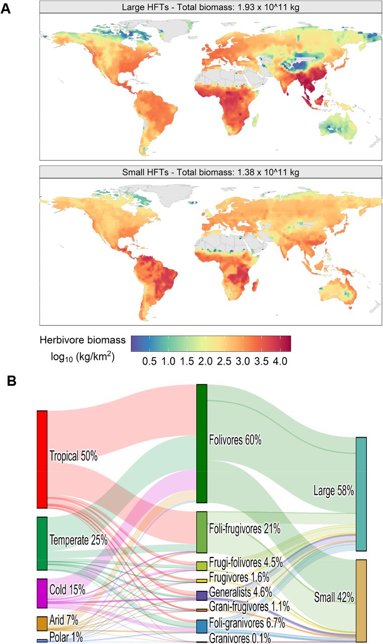
(A) Spatial distribution of modeled biomass under natural conditions (no anthropogenic land cover and no hunting) for the two main mammal size classes. (B) Relative biomass distribution across climate zones (left grouping), diet macro-groups (central grouping), and size classes (right grouping). Climate zones follow the Koppen-Geiger classification (Fig. S3A). Micro HFTs biomass is included in the small HFTs.

Negative residuals indicate modeled biomass is lower and empirical biomass. (A) Spatial distribution of biomass residuals calculated from REMAP output minus the gap-filled empirical biomass (SI Appendix for details on gap-filling of empirical biomass). (B) Probability density of residuals across continents for large HFTs (left) and small HFTs (right)
Small and large herbivores biogeographic patterns were dissimilar (Fig. 2A). Large herbivore biomass was higher in warmer and wetter locations associated with high plant AET (R2 = 0.592), precipitation (R2 = 0.592), and temperature (R2 = 0.334) (Fig. 4F and S6). Instead, small herbivore biomass was more evenly distributed and less correlated to AET (R2 = 0.489), precipitation (R2 = 0.416), and temperature (R2 = 0.173) compared the biomass of large herbivores (Figs. S6-S7). Notable differences in spatial patterns between class sizes were found in the northern cold climates, tropical, and sub-tropical areas. (Fig. 2A, see Supplementary Materials for exceptions and further results). These patterns suggest that, globally, large herbivores are more energy-water dependent than smaller ones, which might be able to extract water from plants through selective feeding8. These conclusions are compatible with previous observations of water-size class correlations in African herbivores13. Outside of Africa, predicted hotspots of large herbivore biomass coincided with human-occupied landscapes: western Europe, southeastern China, central North America, and India (Fig. 2A and Fig. S3C). These elevated human-density areas originally hosted ∼17% of large herbivore biomass and 9% of small herbivore biomass. This implies that rewilding initiatives will be limited in scope in many of these highly productive areas. Globally, the potential decline in biomass due to habitat loss was 42% and 33% for large and small herbivores respectively.

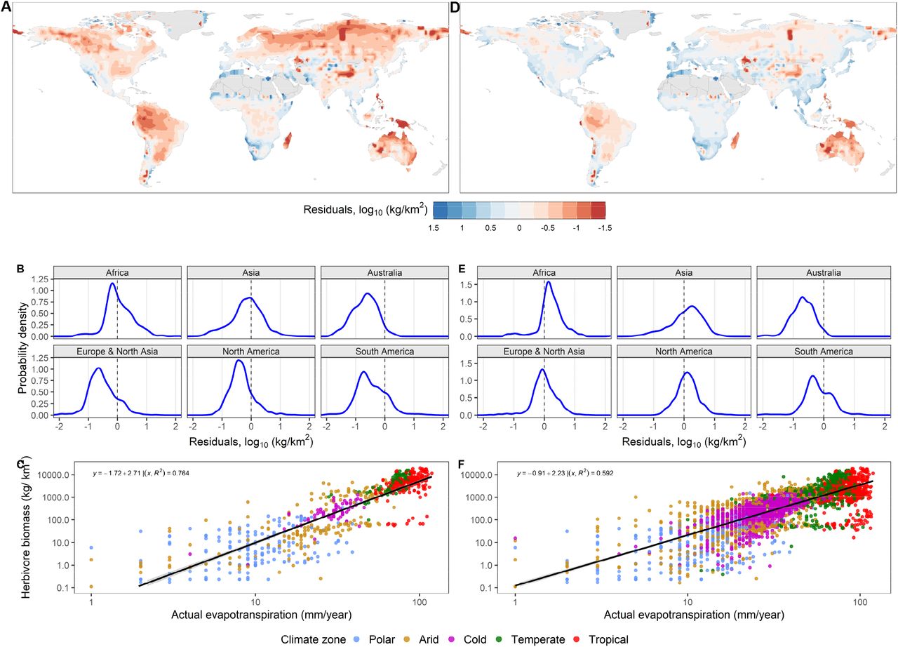
(A & D) Spatial distribution of biomass residuals calculated from REMAP output minus the climate-predicted biomass. (B & E) Probability density of residuals across continents. (C & F) Regression model of AET as a function of modeled large herbivore biomass; Climate-predicted biomass was estimated according to the relation between modeled biomass and climate variables, implying the effects of extinctions. (A, B, C) refer to predictions and data based only on areas where < 20% of megafauna species became extinct. In (D, E, F), the predictions and data are based on the global regression (SI Appendix).
Legacy of Late Pleistocene extinctions
To reveal the fingerprints of Late Pleistocene megafauna extinctions, we used a spatial generalized linear model to predict large herbivore biomass as a function of climate (AET, precipitation, seasonality, and temperature). The model was fitted globally in addition to only areas where the late Pleistocene megafauna extinctions were less pronounced according to extinctions maps we created from distributions of extinct herbivores (25, Fig. S8, and methods). We then used the different fitted models to predicted biomass globally as a pre-extinction estimate and compared it to present-day modeled biomass. The correlation between AET and large herbivore biomass, which was already significant at the global scale (Fig. 4F), was even higher in areas where extinctions were less severe (Fig 4C, S9B, and S9D). This may reflect how potential biomass decreased following the Late Pleistocene extinctions. Specifically, the residuals of modeled minus climate-predicted biomass were predominantly negative in Australia, North and South America, and Northern Asia (Fig. 4A-B). The spatial distribution of the residuals echoes Pleistocene megafaunal extinction patterns (Fig. 4A) illustrated previously in terms of species loss 1. The largest relative loss of biomass occurred in Australia and South America, with 0.5-1.5 order of magnitude difference compared to expected present-day biomass without extinctions (Fig. 4A-B). Residuals are consistent with the extinction of 95% of Australia herbivore megafauna around 45 kyr and South America’s loss of 80% of forest and savanna-dwelling megafauna including ground sloths (Xenarthra), ungulates (e.g., Camelidae, Equidae, and Meridiungulata), and gomphotheres1. Losses of potential biomass in North America and Northern Asia, although more limited, also coincide with extinctions of large ungulates and proboscideans1. In Africa, SE Asia, and western Europe, extinctions were less severe and the model residuals are closer to zero. Without post-industrial habitat loss and hunting, these areas would today host megafauna such as the Asian elephant (Elephas maximum), rhinos, and several ungulates. These patterns are confirmed when the biomass-climate model is fitted in areas with higher extinction rates (Fig. S9A & S9C) and using an independent data set (Figs. S10). These extinction patterns become less pronounced when the biomass-climate model is fitted globally (Fig. 4D-E & S10C-D).
In sum, biomass greatly decreased in Australia and South America and declined in North America and central-northern Asia. These losses of biomass are consistent with previously known extinction patterns and demonstrate an important presence of megafauna in past ecosystems.
Implications for conservation and ecology
High potential biomass of large herbivores overlaps considerably with densely populated regions and croplands. The implications are multiple. In places where rewilding and restoration are desired, our mechanistic model approach provides estimates of the ecosystem capacity to sustain herbivore populations. However, returning to natural biomass levels might only be possible in areas where human use has declined due to abandonment or population decline. In regions struggling with habitat loss and species decline, it offers a carrying-capacity estimate for assessing biomass losses and prioritizing conservation actions. Furthermore, water dependency in mammals important implications for their conservation and should be further investigated given the changes in the global water cycle brought by climate change26.
The ecosystemic role of smaller species is often overlooked, even though many are threatened 27. The first global estimates of small herbivore biomass provided here show that it is a significant component of biomass. Small species likely play an important role in arid and cold regions 28, where water availability is low, or where large mammals are declining rapidly. Thus, small species should receive more attention in studies of ecosystem functioning and biogeochemical cycles.
Mammals in Earth system science
We presented the first global classification of all terrestrial mammalian herbivores (Fig. 1). The HFT system describes the functional diversity of thousands of species using a few key eco-physiological traits. Provided trait data are available, this flexible framework could also be applied to create HFTs for extinct mammals, other endotherms, or ectotherms. The classification provides a new lens for analyzing the mammalian trait space and biogeographic patterns of functional diversity in relation to environmental factors. REMAP is relatively accurate despite the broad spatial resolution and some input limitations (Methods). Finer-scale inputs would improve biomass estimates in highly heterogeneous landscapes such as deserts or arid zones. Still, REMAP is highly accurate in regions containing 90% of the biomass (Fig. 2 and 3). Because REMAP includes competition and functional diversity, it better captures trophic interactions and ecophysiological responses to environmental conditions compare to allometric or statistical models. It, therefore, can show the cascading effects of declines in certain functional groups, of reduction of resources, or of climate change through physiological stress. For example, it could be applied to disentangle the effects of climate change on small and large herbivores26.
The global HFT classification and REMAP lay the foundation for showing how mammals influence biogeochemical cycling, greenhouse gas fluxes, and vegetation dynamics. Our current model does not include all feedbacks between animals and ecosystems, but a foreseeable application would be to couple REMAP with global vegetation models and the inclusion of invasive species and livestock, which today comprise the largest herbivore biomass pool. Further, we envision integration with Earth-system models to demonstrate the influence of mammals in biosphere-atmosphere feedbacks. These will be fundamental steps towards assessing the role of TMH and other animals in ecosystems and climate.
Methods
Methodology overview
Extant mammalian herbivore species were assigned to functional types using hierarchical cluster analysis applied on mammals’ trait data gathered from different sources (Data and Global classification of mammalian herbivores sections). These HFTs were then incorporated in a mechanistic model that simulated the global distribution of pre-industrial (only natural land cover and no widespread hunting) biomass of each HFT as a function of environmental conditions and daily changes in plant biomass availability (REMAP section). REMAP biomass resulted from the HFTs population dynamics and the competition for resources among them. Herbivore biomass was constrained by the availability of food and mortality. Eco-physiological processes in REMAP are described through mathematical equations based on HFT-specific parameters, some of which calculated from body mass allometric scaling. The model results were validated against empirical data of mammal biomass compiled from different sources. Where empirical data were missing, estimates were generated using a linear mixed-effects model (Data section). Climatic variables were used to estimate Late Pleistocene herbivore biomass that was compared to the modeled present-day biomass. We interpreted differences between climate-predicted and modeled biomass as the effect of Late Pleistocene extinctions.
Data section
Mammals’ trait data
We gathered extant terrestrial mammalian herbivore (TMH) species traits data from available datasets: Phylacine (n = 5831), Mammal Diet 2 (n = 6625), Elton Traits (n = 5400), and PanTHERIA (n = 5416) 25,29–31. These datasets do not include semi-domesticated or range species, which were not part of our study. We harmonized taxonomic differences between data sets by using the Phylacine standardized synonym table. These datasets include life-history traits (body mass, diet preferences, longevity, etc.) for all known mammal species. We complemented and verified these data using additional sources from peer-reviewed literature for two key traits in our analysis: digestive system (hindgut or foregut) and folivory type (browser, grazer, mixed-feeder). The main sources used to compile these two traits are given in the following sections and a detailed list is provided in the supplementary data.
Empirical mammal population density & biomass
We compiled a dataset of mammal density estimates from two main sources 32,33 that were complemented with 433 records for a total of 7713 records. The complete list of density data can be found in the appendix. This dataset included 440 species, which represent roughly 50%, 15%, and 7% of the species that we later define as, respectively, large (n = 238), small (n = 108), and micro (n = 94). The mammal density data were collected between 1950-2020 in locations such as national parks or protected areas. The data had geographic and taxonomic gaps as often not all species present in each location were censused. Small and micro mammals had limited geographic coverage and were particularly underrepresented in the data set (Fig. S5). This lack of taxonomic coverage reduced considerably the estimates of total animal biomass per km2 (Fig. S5) and prevented the creation of complete HFT maps (discussed in the following section). We thus generated a complementary 2° resolution gridded dataset for all TMH species using two methodologies: 1) a spatial linear mixed-effects model (LMEM) following 20 and 2) allometric-scaling equations 34. The LMEM was built using the following predictors: body mass, grass and tree NPP from MODIS 35, precipitation of the warmest quarter from WorldClim2 36, and random effects to account for taxonomy and spatial pseudo-replication. In method 2) we used a set of allometric equation to determine density from body mass with slope and intercept that were family and order specific 34. Even though both methods present some shortcomings, LMEMs capture some of the influence of bioclimatic factors on mammal density20. Conversely, allometric equations predict the same density regardless of bioclimatic conditions. We thus preferred to use LMEMs to complement the empirical data as our main benchmark to be compared with the results from REMAP. This seemed sensible as both models incorporate the effect of bioclimatic factors on mammal density estimates. We nonetheless retained the estimates generated from allometric equations as an additional independent measure. We only estimated density in grid cells where species are present in accordance with the Phylacine “present natural” distribution maps 25. Present natural maps are constructed from IUCN maps and represent estimates of presence if there would be no anthropogenic disturbances or pressures and do not account for invasive or introduced species. These natural conditions matched our model simulation conditions (REMAP section). We averaged the empirical data across multiple censuses and occurrences of the same species within each grid-cell. We then combined the LMEM gridded data with the empirical data only where a species was present according to its distribution map but absent in the empirical data. Using the empirical data-LMEM (or allometry) product we derived biomass per km2 by multiplying density by 80% of the body mass reported in Phylacine to account for sexual dimorphism37.
Climate data, megafauna extinction maps, and analysis
We downloaded monthly plant actual evapotranspiration (AET) data from the TerraClimate dataset 38 and calculated yearly average over the period 1958 and 1980. None of the data after 1980 were chosen because we avoided years with elevated CO2 concentrations. We also wanted to approach as much as possible the early 20th century climate data used to model mammalian biomass (see modeling section). Mean annual temperature (MAT), mean annual precipitation (MAP), and precipitation seasonality (PS) were downloaded from WorldClim 2.136, which provides directly the averages. We constructed a linear model of modeled herbivore biomass as a function of these four climatic factors by accounting for the spatial autocorrelation in large herbivore biomass using R package “spdep”. We first performed the Moran’s test to confirm the presence of spatial autocorrelation in biomass. We then computed the spatial autocovariate of (BiomassAC) to be used as a predictor variable in the following spatial generalized linear model:
 Our hypothesis was that the modeled biomass correlation with climate was stronger in areas where the late Pleistocene extinctions where less severe. We identified areas with different extinction thresholds using distribution maps of extinct megafauna25. We calculated the percentage of extinct species in each grid cell and generated three maps with extinction thresholds of 20%, 40%, 65% and a global map (up to 100%) (Fig. Sxx). The thresholds represent the quartiles of the percentage of extinct species. The spatial regression model was applied to the REMAP-modeled biomass in the areas contained in these four maps and the resulting model used to predict biomass globally. As an independent measure the same model was applied to the gap-field empirical data for the 20% threshold map and the global one.
Climate zone data
We generated a map of climate zones using the updated Koppen-Geiger climate classification 39. We aggregated the original classification into the five top-level climates: tropical (equatorial), arid, temperate, cold (snow), and polar.
Artificial habitat data
We created a map of anthropogenic areas by aggregating at 2° resolution the artificial habitat layer of a global map of terrestrial habitats 19. In the original map the artificial habitat included urban areas, plantations, and agricultural lands but not rangelands because they are not present in the IUCN habitat classification scheme. Thus, our estimate of artificial habitat in each cell might be underestimated. We classified grid cells as “human dominated” if the fraction of the artificial habitat within a cell was higher than 50% (Fig. S3C). We assumed that 100% of herbivore biomass in human-dominated cells is lost because even if small fractions of natural habitat persist, they are probably too fragmented to host any substantial populations. Contrarily, unrealized biomass in non-human-dominated cells was calculated by multiplying modeled biomass by the fraction of artificial habitat. We thus assumed that non-human-dominated cells keep hosting functional habitats.
Global classification of mammalian herbivores
We used Phylacine as our taxonomic and diet reference database, as it is the most recent database and uses phylogeny to better estimate species diet composition 25. We selected all terrestrial species whose diet is composed of at least 80% plant material (n=2947) from which we excluded nectar feeders (≥ 20% of nectar in diet, n=78, average body mass 0.190 kg). Nectar feeders were excluded because nectar is not simulated in vegetation models and thus their food availability could not be calculated (see next paragraph for more details). Species with a low percentage of nectar in diet (< 20%) were instead retained. We also excluded species classified in Phylacine as extinct (extinct in prehistory or after 1500 CA, n= 267, average body mass 613 Kg). We grouped the six (fruit, seed, leaf, root, nectar, and “other”) diet-preference categories of Elton Traits (ET) and Mammal Diet 2 (MD2) into three (fruit, seed, and leaf). We added the percentages of root and “other” to leaf and added nectar to fruit for the few species who had 5-15% nectar in their diet. Fruit, seeds, and leaves represented the vast majority of TMH’s diet. Less than 5% of all the species we selected had root, “other”, and nectar in their diet. Within these species the average values of root (11%), “other” (10%), and nectar (0.2%) were low and thus these plant parts had little importance on the overall diet of the selected TMH species. In vegetation models, leaves are frequently simulated in large-scale simulations whereas fruit and seed production is calculated based on simple parameterizations. Fruit and seeds processes are however simulated with more detail in small-scale vegetation models 40. Regardless of their implementation in models, leaves, fruit, and seeds all had to be considered as they represent key components in TMH diets and ecology. For each species, we determined diet composition (in percentage) based on the diet source indicated in Phylacine, which was in most cases either ET or MD2. If the diet source was MD2, we rescaled the original MD2 values (0-3) to 0-100%. For species (n=210) in Phylacine whose diet source was neither ET nor MD2, we first searched in ET and MD2 for any matching species whose diet was determined at the species level. If we did not find a match, or if diet was determined at the genus level or above, we manually assigned diet preferences following literature. As a last resource, we used the genus average. We then assigned to each species a digestive system (hindgut or foregut) and a folivory type (grazer, browser, mixed-feeder). We referred to a published dataset to determine digestive system 41, if we did not find a match at the species level, we used the genus and finally the family. We only used genus or family when all species within the taxonomic rank had the same digestive system, otherwise we referred to primary literature (complete list in supplementary material). We determined folivory type starting from species identified previously 42, which we updated with articles published after 2013 (complete list in supplementary material). All other species’ folivory type were assigned based on primary literature or following the genus to family strategy used to determine digestive system.
We then applied hierarchical cluster analysis (R package “factoextra”) using as data input the three plant organs. We evaluated results produced by several clustering methods: hierarchical (“.D2”, “average”, “agnes”) and kmeans (“kmeans”, “pam”, “fanny”). We settled on “agnes” as it provided the tightest clusters that were evaluated using silhouette width (average distance between clusters), Dunn index, and standard deviation. We found eight to be the optimal number of clusters (dietary macro-groups) based on statistical evidence and ecologically meaningful diet types. These groups were: Leaf, Leaf & fruit, Fruit & leaf, Fruit, Leaf & seed, Seed & fruit, Seed, and Generalist (Fig. 1). Less than 5% of all species were at the edges of each cluster (negative or low silhouette width). These species were reassigned to the group with the most similar dietary preference. This process improved the clusters compactness by increasing the silhouette coefficient and reducing the standard deviation of diet components. A second level of grouping was made by splitting the eight macro-groups in micro (mean 0.13 kg, range 0.004-0.05 kg), small (mean 1.6 kg, range 0.05-10 kg) and large (mean 92.4 kg, range 1-4400 kg) animals, only the Seed group (Granivores) did not contain large species. This was necessary because body mass in mammals spans various orders of magnitude and underlies significant eco-physiological differences such as longevity, litter size, and litter per year. We used change-point analysis to determine significant differences in mean body mass among species in each diet group. Change-point analysis is a technique used to detect trend changes in timeseries but when applied to ordered data 43 it helps identify groups having similar mean values. Along with the results from the change-point analysis, we also considered biologically-relevant information, such as taxonomy, to minimize arbitrary species assignments. The size threshold was determined for all species within each macro group (Fig. S1C). Consequently, the thresholds of each size class vary in each diet group and overlap slightly among size groups. Micro HFTs differed from small HFTs in body mass; whereas diet composition, digestive system, and folivory type were the same. In REMAP simulations, micro mammals biomass was only 5% of the total biomass. Thus, their simulated biomass was added to the biomass of small HFTs to simplify the presentation of the results. Finally, a third grouping was made within the size groups according to their digestive system and folivory type. These two key traits dictate, among other features, maximum daily intake (eq. 1 and 2 shown later) and type of leaf consumed (grasses, trees, or both). Non-ruminant foregut fermenters were treated as foregut fermenters because fermentation takes place in the same part of the stomach and specific model parameters for non-ruminants were not available44. Creating one HFT for each combination of these two traits within each diet-size group would have generated a large number of HFTs. Instead, we identified the most common combinations of digestive and folivory type using two metrics: number of species and geographic range (number of grid-cell occupied). Because more than 85% of species were hindgut fermenters, folivory type was the main trait we used to assign species to specific HFTs within dietary-size groups. We used digestive system mostly to distinguish large folivore HFTs. Some species were assigned to HFTs with a different folivory type but we avoided assigning grazers and browser to the same group as much as possible. As a compromise, some browsers or grazers were assigned to mixed-feeders HFTs. At the end of this multi-tiered grouping each species was assigned to an HFT (list of species in data S1). Each HFT could then be described in terms of (Table S1A): 1) diet composition (percentages of leaf, fruit, and seed in diet) determined by the average of all species within each HFT; 2) size class (large, small, and micro); digestive system (hindgut or foregut); 4) folivory type (only for obligate or partly-folivores). In total we had 11 and 13 HFTs for large and small herbivores respectively.
REMAP: a mechanistic model of herbivores ecophysiology
REMAP is mechanistic model that simulates ecological, physiological, and demographic processes of different HFTs competing for food. These processes are described with mathematical equations partly based on a previous model 45 which simulated large grazers as a single HFT and was integrated in the ORCHIDEE model (described below). In the Zhu model, maximum energy intake and energy expenditure were calculated based on physiology, body mass scaling, and temperature. Grazers consumed the available grass simulated by ORCHIDEE and converted the energy surplus into fat storage. Grazers prioritized feeding on fresh leaves otherwise they resorted to eating litter or starved if no food was available. Fat storage determined annual birth rates and influenced mortality rates because fat was converted to energy during periods of starvation. Conceptually, fat storage was used as a proxy for energy stored in tissue that is mobilized to perform different functions. In reality, other tissues such as muscles and bones are mobilized during starvation and reproduction but fat is the primary one46,47. The effect of predation was not explicitly modeled but was captured by using a carrying capacity parameter in a logistic equation. The structure of most equations in REMAP remains unchanged from the Zhu model. However, we recalculated most equation parameters to accommodate for the wide variation in eco-physiology within the new HFTs (Tables S1A, S2-S3). The recalculated key parameters include: maximum fat storage, aging mortality, establishment rate, daily intake and food energy content, carrying capacity, and energy expenditure (Table S2). Competition for food among HFTs and flexible diets are key added features along a new establishment scheme to account for small species breeding frequently throughout the year. Here we provide a brief overview of the processes already present in Zhu et al. 45 and describe the novel mechanisms and parameterizations.
Model setup
REMAP inputs are gridded time series of plant material (leaf, fruit, and seed) turnover and maps of HFT body mass. The simulations length was 300 years at 2° spatial resolution and REMAP output consists of time series of population densities (individuals/km2) for each HFT. Densities were averaged over the last 50 years of the simulation because populations can fluctuate over time due to demographic and ecological processes. Densities were then multiplied by HFT body mass to obtain live biomass weight (kg/km2) for each HFT at 2° degrees resolution.
Daily intake and food energy content
Following 44, the maximum daily energy intake equation is:
 where Imax (MJ d−1 ind.−1) is the maximum daily net-energy intake per individual, W is the individual body mass (kg), and d is the percentage of dry matter (DM) set at 70% for fresh plant material and 40% for litter. Parameters i, j, and k are determined by the folivory type and digestive system of each HFT following (Values in Table S2) 44. Because mixed-feeders were not contemplated in 44, we calculated i,j, and k as the average between the values for browsers and grazers. Imax is constrained by maximum fat (explained later). We acknowledge that different estimates of mean retention (gut passage) time might lead to different maximum daily intake than the ones in eq. 1, particularly for hindgut fermenters lighter than 100 kg48 or for other types of mammals such as frugivores. However, we only found one reference providing separate i,j, and k parameters for a few different herbivore types44. In the future, specific parameters should be developed for other types of herbivores such as frugivores and granivores for more accurate calculations of daily intake. We derived the maximum-daily intake in dry mass (kgDM d−1 ind.−1) by dividing Imax by the net energy of food following49:
 Where NE (MJ kgDM−1) is the net energy calculated from metabolizable energy (ME) using the conversion formula NE = ME x (0.503 + 0.019 x ME) 49. NE varies for each HFT based on the type and percentages of plant material in the diet (Table S3). We thus calculated NE for HFTs eating multiple plant organs with a weighted average based on the percentages of each plant organ in the diet (Table S3).
 Where NEorgan are the average values of diets of various mammals based on the metabolizable energy content of those diets for: MEgrass (11.2 MJ kgDM−1)50, MEbrowse (10.0 MJ kgDM−1)51, MEseed (16.9 MJ kgDM−1) 51, and MEfruit (8.4 MJ kgDM−1)52; and forgan is the fraction of each plant organ in the diet, the sum of all forgan is 1. Thus, MEorgan already accounts for differences in fiber and protein contents among diets and their digestibility.
Flexible diet
The food mix ratio of each HFT is shown in Tables S3. Because herbivores show a certain degree of flexibility in their diet, they can change their food mix ratio if the ideal ratio is not attainable. For example, we set the ideal food mix ratio of Folivores mixed-feeders to 50% grass and 50% browse. However, when either grass or browse is scarce, mixed-feeders can eat more of the other type within a certain limit. Lower and upper bounds for each HFT were determined based on results from our cluster analysis (Fig. S1). The main idea was to keep distinctive diet preferences for each HFT while providing some diet flexibility.
Energy expenditure
Daily energy expenditure (MJ d−1 ind.−1) is calculated with the following equation:
 The k1 and k2 parameters were introduced by 45 to account for the effect of long-term mean air temperature (T) on metabolic rate. We used a variable k3 parameter to account for differences in the slope of the body mass-metabolic rate relationship among different mammal orders. We estimated k3 by first assigning to each species a slope value according to its order 53. We then calculated an HFT-specific slope by averaging all its species slope weighted by the number of grid cells where each species was present (slope values in Table S2). The weighted average was used to avoid skewing the average slope in favor of narrowly-distributed species.
Maximum fat mass
The maximum fat storage per individual (Fmax, kg ind-1) is used to limit the actual daily intake so herbivores cannot exceed their Fmax (equations 5a and 5b). Maximum fat storage also determines the maximum yearly birth rate (equation 7) and influences mortality rates due to starvation (described below). Fmax was originally set to 30% of body mass in 45. However, fat storage scales allometrically to body mass, and to cover the broad range of body mass across HFTs we used an allometric scaling equation so that Fmax = 0.075 x W1.19 54.
Actual daily intake
the actual daily intake I (MJ d -1 ind.-1) equation follows 45. Actual daily intake is calculated first by determining the feeding requirements for each HFT population by multiplying IDM,max by HFT population density P (individuals km-2), which is initialized at 0.001. Population feeding requirements are then compared to the available biomass pools and IDM,max is calculated according to the different percentages of biomass pools consumed. Folivores and partly-folivores can consume litter when fresh leaves are not available whereas granivores and frugivores only rely on fresh plant organs.
 Where F is the fat storage per individual (kg ind-1) and m is the conversion coefficient between fat and energy (eq. 6). m = 39.3 when I < E and m = 54.6 when I > E 55. E is calculated in eq. 4. Conversion between energy and fat: changes in fat storage are calculated daily following 45

Birth and mortality rates
the maximum yearly birth rate (Bmax, yr -1) is defined following 55
 Where r = 15.16 − 2.25 × log10(W × 1000) is the population rate of increase. We used a linear regression to derive r (litter size times litters per year) as a function of body mass from trait data 29. We assumed a 1:1 sex ratio in the population so r is multiplied by 0.5. Bmax is calculated daily and its yearly average is used to calculate the actual annual birth rate (eq. 8). The actual birth rate B (yr-1) also depends on fat storage and is calculated by accounting for the energy invested during reproduction:
 Equations 7 and 8 were originally parameterized for large herbivores producing on average less than one offspring per year 45. We thus implemented a modification for smaller animals who give birth to several offspring per litter. For HFTs with W < 10 kg B = Bmax if Fmax is reached during the year, otherwise
  . After reproduction, the fat invested for giving birth
  is subtracted from F or, only in the case when HFTs with W < 10 kg reach Fmax, F is set to 0. We acknowledge that income breeders might be less dependent on fat storage and thus might follow a slightly different scheme.
Mortality rate
animals are subject to three types of mortality: aging mortality (Ma, yr -1), starvation mortality (Ms, yr -1), and density-dependent mortality (Md, yr -1). In the Zhu model, Ma was a fixed parameter defined as the inverse of maximum longevity. As longevity is positively correlated with body mass, we used a linear regression model of log-transformed data to estimate Ma as a function of body mass using empirical data on maximum longevity 29.
 Ms represents the increase in mortality due to prolonged starvation. Ms is implemented following 45,55 and is calculated daily as the probability of fat to be below a threshold Fthresh set at -0.2 × Fmax45. Fthresh allows to implicitly account for cold-climate behavioral and physical defences56 that allow herbivores in colder climates to endure longer periods of starvation. Density-dependent mortality is controlled by a function through which a theoretical maximum population
  is reached only given optimal conditions (no starvation mortality, maximum birth rate, and minimum aging mortality) over an infinite time. The kd term in eq. 9 is the slope of this density-dependent function and is calculated globally for each HFT using its maximum observed density. The theoretical maximum P is not reached in REMAP simulations, as optimal conditions are not always satisfied and time is not infinite. Thus, kd does not have an important role in any emergent results of the model, but it is still useful to account for processes that influence population growth rate that were not explicitly simulated. For example, to implicitly include the effect of predators and other processes limiting infinite population growth such as self-thinning (i.e., pathogens).
The population dynamics are controlled by:
 P is initialized to 0.001 ind. km-2 and is updated yearly. When P falls below 0.001, P is reinitialized to 0.001 and F is set to 0.
Competition for food
multiple HFTs can be present in the same grid cell and might compete for the same food type. To resolve this resource-acquisition conflict, we implemented a semi-random procedure that determines the order in which HFTs feed at each time step. The order of access is given by a random number generator multiplied by a weight which is a function of HFT body mass. The weight for each HFT is determined by first dividing 100 by the number of HFTs present in each grid cell (Vavg = 100/Nhft). Vavg is the average weight equal for all HFTs. The heaviest HFT is then assigned a weight equal to Vavg + Vavg x 0.01, which represents a 1% higher chance of being the first to feed compared to the average. The second largest HFT is assigned Vavg, the third Vavg -Vavg x 0.01, the fourth Vavg -Vavg x 0.02, and so on. The third largest animal has -1% chance of the average of being the first to feed, the fourth largest has -2% chance, and so on. This approach maintains some randomness while trying to consider that heavier species might have priority over lighter species when accessing the same resources 57. Since this assumption has not been fully documented, we maintained a fairly conservative approach by giving to the heaviest HFT only a 1% higher probability of feeding first.
REMAP gridded inputs
REMAP spatial resolution is determined by the resolution of its inputs, notably: a) time series of production and turnover rate of plant organs and b) HFT body mass maps.
Time series of production and turnover rate of plant organs can be derived from remote-sensing products or from the output of vegetation models. For our simulations we generated a 300-year time series of plant organs at 2° resolution using the ORCHIDEE (Organizing Carbon and Hydrology In Dynamic Ecosystems) vegetation model 18. ORCHIDEE provides net primary productivity (NPP) allocation and turnover rate at a daily time step containing the following plant organs pools: fresh leaves and litter from grasses and trees, fruit, and seeds (see data section for full description of ORCHIDEE). Even though our simulations are not fully coupled, the available biomass pools are updated daily to account for animal consumption, NPP allocation and turnover rates. In a fully-coupled simulation (REMAP & vegetation model), the feedbacks between animal and plants would allow a more precise estimation of the available biomass pools. For example, the removal of leaf biomass would change water use and carbon allocation of plants.
Body mass is a prescribed input in REMAP because many processes scale accordingly to. The body mass of each HFT varies spatially because not all species assigned to an HFT are present in all grid cells within the HFT range. We generated global maps of HFT body mass at 2° spatial resolution to match the spatial resolution of ORCHIDEE. The gridded body mass maps were created according to the “present natural” distribution maps previously described (Fig. S2). The actual body mass of each HFT was the average of all HFT-species present in a grid cell weighted by their density in the same grid cell (individuals/km2).
Description of the ORCHIDEE vegetation model
The time series used as input for the REMAP simulations was generated from the vegetation model ORCHIDEE version 2.1 based on 18. ORCHIDEE is a process-based model that simulates vegetation dynamics and plant eco-physiology (photosynthesis, phenology, growth, allocation, and mortality) through equations describing energy and water exchanges with the environment. Environmental conditions are determined by time series of climatic forcings (temperature, humidity, precipitation, and radiation) and by soil properties. Plant diversity is organized in plant functional types (PFTs), which are group of species with similar physiological and life-history traits. In ORCHIDEE 2.1 there are 15 PFTs that cover tree (broadleaf and needleleaf) and grass (C3 and C4) functional diversity across biomes (PFT names in18). Each PFT is defined by a set of parameters related to photosynthesis, allocation strategies, and physical traits (most notably leaf traits). PFTs compete for space, water, and light and coexist in the same grid cell by occupying a prescribed fraction of the cell. ORCHIDEE keeps track of a large number of biomass and carbon pools above and below ground. Processes are simulated at various time steps from hourly to daily. After an initial spin up simulation to reach equilibrium in the carbon pools, a 300-year time series was generated by cycling through climate forcings from the years 1900-1950. The simulation included 13 PFT distributed according to a reconstructed land cover of ∼1500 YBP. Crops were excluded because we simulated conditions in natural settings. The land cover map was created by merging the ESA CCI dataset (https://www.esa-landcover-cci.org/) and the LUH2 dataset (http://luh.umd.edu/). The ORCHIDEE simulation had a spatial resolution of 2° and was forced with CRU-NCEP six-hourly climate data 58, re-interpolated to the 30-minute time step used by ORCHIDEE. In the time series used as REMAP input we made a distinction between the availability of browse and grass biomass: 100% of grass-leaf biomass was available for consumption instead only 20% of tree-leaf biomass could be consumed. In forest ecosystems only a fraction of leaf biomass is available or preferred for consumption. Only the understory leaf biomass is available to terrestrial herbivores and arboreal folivores consume mostly fresh leaves, which are highly digestible and represent a small percentages tree-leaf biomass. The 20% estimate is based on reported leaf understory biomass 59– 61 and was assumed to include twigs, bark, and small shrubs, which are not explicitly simulated in ORCHIDEE. In ORCHIDEE 10% of NPP is allocated to fruit but there is no distinction between fruit and seeds. We thus split fruit biomass in equal parts assigned to separate seed and fruit pools, although we acknowledge that conifers do not produce fruit and might invest more in seeds. Most litterfall studies do not distinguish fruit and seeds making it challenging to establish an appropriate ratio 62.
The biomass pools for leaves (browse & grass), fruit, and seeds are a critical input as they determine the availability of food for HFTs. These pools are related to ORCHIDEE’s NPP which is allocated to different plant material. ORCHIDEE’s NPP has been validated before but has not yet been evaluated for its capacity to simulate leaf, fruit, and seed biomass. As no large-scale datasets of leaf biomass were available, we compared tree and grass NPP from ORCHIDEE against Moderate Resolution Imaging Spectroradiometer (MODIS) NPP 35. This comparison was only a proxy to validate leaf biomass, as the ratio of NPP assigned to leaves in ORCHIDEE is not constant. ORCHIDEE generally underestimated NPP (Fig. S4). Notably, underestimation was very marked in arid and polar climate zones where ORCHIDEE’s NPP was frequently less than half compared to MODIS (Fig. S4C). In temperate and cold zones ORCHIDEE’s NPP was slightly closer to MODIS compared to arid and polar ones. Tropical areas showed the highest agreement between ORCHIDEE and MODIS (Fig. S5C). However, the overall spatial patterns of NPP were similar between the two models (Figs. S5A-B). This implied that leaf biomass availability followed these general patterns in the REMAP input. To validate ORCHIDEE fruit production we collated various data sets of fruit fall for a total of 81 observations across different forest types 62,63. In areas where more data points were available, ORCHIDEE’s over-estimated fruit NPP by a ratio of ∼1.5 compared to empirical data (Fig. S4D). We observed under-estimation mostly in sites from African and Oceania forests but samples size for these regions was low (n = 8). We corrected this estimation by reducing the availability of fruit and seed in the REMAP input.
REMAP validation data
We validated REMAP output against the gridded product of gap-filled empirical density described in the data section. We calculated the mean average error (difference between modeled and empirical biomass) and normalized it using the average biomass of each HFT. Normalizing the mean average error makes it possible to compare model results across HFTs as their average biomass spans several orders of magnitude. We also calculated the residuals by subtracting the gap-filled empirical biomass from the REMAP-modeled biomass.
Author contributions
F.B. obtained the funding. F.B. conceived the project with input from P.C. F.B. develop the methodology with input from all other authors. F.B. performed the analysis and prepared the figures. F.B. led the writing and all other authors contributed with editing and feedback.
Competing interests
Authors declare that they have no competing interests.
Supplementary Information is available for this paper
Acknowledgments
We thank J. Chang, C. Doughty, and M. Clauss for constructive comments and feedback on a previous version of the manuscript, Y. Hui for providing MODIS data, F. Maignan, M. Peaucelle, and N. Viovy for the assistance with ORCHIDEE, P. Stevenson for help with fruit production, and L. Santini for the help with linear mixed-effects model setup. F.B. was supported by European Union’s Horizon 2020 research and innovation program under the Marie Sklodowska-Curie grant #845265.
Methods references


