

Abstract
Tissue specimens taken from primary tumors or metastases contain important information for diagnosis and treatment of cancer patients. Multispectral imaging allows in situ visualization of heterogeneous cell subsets, such as lymphocytes, in tissue samples. Many image processing pipelines first segment cell boundaries and then measure marker expression to assign cell phenotypes. In dense tissue environments such as solid tumors, segmentation-based phenotyping can be inaccurate due to segmentation errors or overlapping cell boundaries. Here we introduce a machine learning pipeline design called ImmuNet that directly identifies the positions and phenotypes of immune cells without determining their exact boundaries. ImmuNet is easy to train: human annotators only need to click on immune cells and rank their expression of each marker; full annotation of tissue regions is not necessary. We demonstrate that ImmuNet is a suitable approach for immune cell detection and phenotyping in multiplex im-munohistochemistry: it compares favourably to segmentation-based methods, especially in dense tissues, and we externally validate ImmuNet results by comparing them to flow cytometric measurements from the same tissue. In summary, ImmuNet performs well on diverse tissue specimens, takes relatively little effort to train and implement, and is a simpler alternative to segmentation-based approaches when only cell positions and phenotypes, but not their shapes are required for downstream analyses. We hope that ImmuNet will help cancer researchers to analyze multichannel tissue images more easily and accurately.
Introduction
Tissue samples provide key information about the manifestation and progression of many diseases. In clinical oncology, histopathological examinations serve as an important basis for cancer diagnosis, treatment response monitoring, and relapse detection. There are also intensive ongoing efforts to develop histological biomarkers for selecting the appropriate treatment for cancer patients. Traditionally, tissue specimens are evaluated manually by trained pathologists, but machine learning systems are increasingly being developed for automating some aspects of tissue evaluation and improving the objectivity, reproducibility, and scalability of these aspects of histopathology.
A core task of histopathological analysis is the localization of different types of cells. Many types of cells, such as epithelial cells and cancer cells, can be accurately identified based on morhopological aspects like size, shape, or nuclear atypia. White blood cells, however, differ little in morphology and need to be identified based on the expression of marker proteins. Such cells come in many flavours that require combinations of multiple markers for proper identification; for instance, T cells alone can be grouped in up 10 major subsets, several of which can be subdivided further [1]. Accurate identification of such immune cell subsets is critical in the context of immuno-logical diseases or immunotherapies – different immune cell subtypes perform very different functions within the tumor microenvironment. To allow in situ mapping of immune cell subsets, several multiplex imaging techniques such as multiplex immunohistochemistry (mIHC) [2], co-detection by imaging (CODEX) [3], cytometry by time of flight (CyTOF) [4], or NanoString’s digital spatial profiling [5] have been developed. All these techniques de-liver multi-channel images that typically consist of a nuclear stain (such as DAPI in mIHC) together with nuclear, cytoplasm, or surface markers to identify cell locations and phenotypes.
Computational analyses of multiplex data often start by segmentation – partitioning the pixels in an image into multiple cells or background. After cell locations and shapes have been identified, one can then measure the expression of each cellular marker by integrating its signal across all pixels belonging to the same cell. Variations of this approach are based on a more fine-grained subsegmentation of each cell into, for example, nucleus and membrane components; this allows to more accurately measure the expression of markers localized to that component of the cell.
Cell segmentation is a notoriously difficult problem in biomedical image processing, especially in dense tissue specimens [6]. The biomedical imaging community has devoted significant efforts to cell segmentation, which has been the subject of several benchmark datasets and algorithm competitions. However, even near-perfect segmentation algorithms are affected by the fundamental issue that cells in dense tissues may overlap. Strategies to address this problem include dissolving the tissue [3], which however loses important spatial information, and post-hoc corrections of expression profiles similar to compensation approaches in flow cytometry [3]. In this paper, we take a fundamentally different approach: we develop a segmentation-free pipeline that treats cell localization and phenotyping as one integrated problem, and does not rely on segmentation as an initial step. We propose a machine learning architecture to tackle this problem and show that our approach achieves accurate results while being considerably easier to implement and train than segmentation-based pipelines.
Results
Segmentation-based phenotyping fails in dense tissues even when segmentation is perfect
Cell segmentation is a well-studied problem in biomedical imaging [7]. In recent years, traditional approaches to cell segmentation such as the Watershed algorithm [8] are becoming gradually superseded by machine learning [9]. For instance, in our experience, the recently proposed StarDist architecture [10,11] achieves excellent performance. Existing cell phenotyping pipelines typically start with cell segmentation as their initial step, and then evaluate marker intensities to assign a phenotype to each detected cell. This is sometimes done by simple thresholding of marker expression [12], but classifiers based on multiple features are also in use. Despite these technological advances, cell segmentation in multispectral imaging is still broadly considered a challenging problem [3,9]. Issues that complicate both segmentation and phenotyping include: spectral unmixing effects, where channels are not separated well from each other; steric hindrance, where cells that are already stained with one antibody become less efficient targets for subsequent antibodies [2]; and high tissue density that leads to overlap between adjacent cells even in thinly cut slices. Classic segmentation algorithms assign each pixel to one cell (or background) and are therefore not well suited for dense tissues, whereas StarDist, for instance allows for pixels to belong to multiple cells.
To assess the need for developing a segmentation-free analysis pipeline instead of building on existing segmentation-based approaches, we analysed multispectral images generated by a computer simulation model. Unlike real images, such in silico generated images have an available “ground truth”: we exactly know to which cells each pixel in the image belongs. Therefore, we can use such images to reason about the hypothetical situation in which we have a perfect segmentation algorithm available, which helps us to put an upper bound on the performance that any such approach can achieve.
To mimic real fluorescent histopathological images as closely as possible, we used the Cellular Potts modeling framework [13–15]. We placed “labelled” cells of realistic size (about 5-10μm in diameter) into a 3D space representing an unlabelled background structure, and cut out thin slices of 4μm depth (Figure 1A). We then simulated noisy expression of nuclear, cytoplasmic, and membrane markers on these cells and integrated the expression values along the Z axis to obtain simulated 2D multispectral images, which indeed had a striking similarity to real multispectral images (Figure 1A,B).

(A) To generate artificial immunohistochemistry images, we simulated cells at different densities within a 1283 μm3 volume, and cut 4μm thick in silico slices spaced 8μm apart. (B) Simulated tissue slices and corresponding scatterplots of CD3 and CD20 expression on perfectly segmented cells at low and high cell densities. (C) At high density, individual cell populations are no longer identifiable (10% density: ~3,000 cells/mm2; 100% density: ~30,000 cells/mm2). (D) Compared to membrane-expressed markers (left), markers expressed in the entire cytoplasm (right) are less affected by noise and spillover from adjacent cells.
As expected, we found segmentation-based phenotyping to work very well at low cell densities. Simple flow-cytometry-like scatterplots of marker expression robustly identified separate cell populations, which would be easy to classify in downstream analysis. However, at densities where cells overlapped, the separation between the different populations on the scatterplot disappeared, creating the appearance of a single population with a continuum of expression of both markers (Figure 1C). While it would still be possible to place arbitrary thresholds on these expression values to extract subpopulations, this approach would now either risk ignoring a substantial proportion of the cells, or misclassifying cells in the “double-positive” area. The problem was alleviated but not eliminated when we considered cytoplasm-based markers, which are less affected by cell overlap (Figure 1D).
In summary, our simulated data demonstrate that even if a perfect cell segmentation algorithm was available, segmentation-based phenotyping would still be difficult in dense tissues where expression readouts, especially of membrane markers, spill over between adjacent cells. While such spillover effects can be partly corrected in post-processing [3], here we opt instead to design an image processing pipeline that is designed to treat cell phenotyping as a first-class problem instead of a downstream step of cell segmentation.
An artificial neural network architecture for no-segmentation phenotyping
In this paper, we focus on cell detection and phenotyping for multiplex immunohistochemistry (mIHC) imaging of formalin-fixed paraffin-embedded (FFPE) tissue. Specifically, we employ mIHC using the Opal tyramide signal amplification (TSA) technique and multispectral imaging [16]. When used in conjunction with the Vectra 3 system, this method can combine 6-7 markers within one FFPE tissue section. However, because of the serial staining protocol, panels have to be optimized carefully [2]. Using this technique, we developed a seven-color lymphocyte panel to detect different lymphocyte populations within tissue consisting of CD3, FOXP3, CD8, CD45RO, CD20, a tumor marker (such as pan-cytokeratin or melanoma specific antibody cocktail), and DAPI (Figure 2A).

(A) Multiplex immunohistochemistry imaging using a DAPI nuclear stain and a 5-marker panel designed to identify cytotoxic (CD8), regulatory (FOXP3) and memory (CD45RO) T cells (CD3) as well as B cells (CD20). (B) “Click” annotations of the locations of two cells and one background annotation (no cell). (C) “Decorations” of the annotations shown in (B) specifying the annotator’s certainty that each marker is expressed or not on the corresponding cell. (D) ImmuNet architecture consisting of 9 convolutional layers arranged in 3 blocks with skip connections, followed by a convolutional layer to reduce feature map size to 3×3, a fully connected layer and 2 output branches of a fully connected layer each. The network is trained on 63×63×6 input images and generates 3×3 output matrices containing the distance to the nearest cell (proximity branch) and the expression of each marker on the nearest cell (pseudomarker branch). (E) Output of the ImmuNet network on the input shown in (A). White circles show cell positions detected by Laplacian of Gaussian post-processing of the proximity map.
In previous studies [2,12,17,18], we used the software inForm (PerkinElmer) in conjunction with in-house developed downstream quality control and analysis software [2] to segment and phenotype cells in mIHC images. Given our familiarity with this pipeline and our experience in fine-tuning it to specific tissues, we use it through-out this paper as a baseline method for comparison. The inForm software uses a machine learning algorithm to assign every pixel in the image to at most one cell, and subdivides each cell into “nucleus” and “membrane” segments. Subsequently, it extracts marker expression information for each channel (e.g., mean expression, range of expression, variance of expression) along with morphological features such as size and shape indices. Users can manually annotate cells with known phenotypes to train a multinomial logistic regression classifier model that assigns a phenotype to each cell [19]. As we will show, this approach works quite well at low cell densities, as long as the software parameters are appropriately tuned. However, as we will also show, the performance of this approach is not satisfactory in dense tissue. Unfortunately, especially immune cells are often found in densely packed structures such as secondary lymphoid organs or tertiary lymphoid structures.
The first step to developing machine learning pipelines for computer vision is to formulate the problem in terms of the desired input and output. Existing neural network architectures for cell segmentation are typically based on input images where a user has manually drawn in the outline of every cell. Generating such full shape annotations is a time-consuming task. While sparse tissues are easier to annotate, networks trained on such images may perform poorly on dense structures they have not seen during training. For these reasons, we designed a machine learning architecture with two key design goals in mind: (1) users should only have to annotate the location of each cell (click annotation) instead of its entire shape (polygon annotation), given that we do not intend to use the shapes anyway; (2) users should not have to annotate training images fully, because even for a human expert it can be difficult to identify every cell in dense tissues. We therefore developed a custom annotation tool that allows users to place annotations simply by clicking on the center of cells of interest (Figure 2B). In a second step we call “decoration”, users can verify and finetune the locations of the annotated cells and rank the expression of each phenotyping marker on a five-point Likert scale (Figure 2C). Importantly, the Likert scale represents the user’s certainty that a cell expresses or does not express a certain marker rather than a qualitative judgment on expression intensity. This allows annotators to specify that they are uncertain about some cases, which can then be resolved by discussing these cases in a larger team of annotators and getting input from experts.
We then designed an artificial neural network (ANN) architecture that processes the location and phenotype annotations to generate two types of output per pixel: (1) the proximity of this pixel to the nearest center of a cell; (2) the expression of each phenotyping marker on the nearest cell (Figure 2D,E, Table 2). The network has a fully convolutional structure (Figure 2D, Table 2) that allows it to generate whole-image predictions during inference despite generating only small patches of output during training (we use a patch size of 3×3 pixels to encode at least some information on the smoothness of the proximity function). This setup makes it straightforward to process sparsely annotated data: only pixels in close proximity to annotated cells are considered during training. To be able to distinguish background and foreground, we also allow users to place special annotations into regions that do not contain any cell of interest. Our ANN architecture is loosely based on the DeepCell network [9] and incorporates a key idea of Wang et. al. [20], who trained a network on distance transformation of cell locations.
In all convolutional and max pooling layers stride 1 is used.
Hence, our ANN architecture, which we call ImmuNet, generates maps that encode information about cell location and phenotypes, but not cell shape. These maps can be processed further using any object detection algorithm. We found a simple Laplacian of Gaussian (LoG) blob detection algorithm to work well for our purposes (Figure 2E). Combined with LoG, the ImmuNet outputs a list of spatial coordinates of each detected cell and its expression of each marker quantified by what we call “pseudomarkers” (ψ). This kind of data is familiar to many biologists as it closely resembles the output of flow cytometers, but with added spatial information. Indeed, we found that converting ImmuNet data to the flow cytometry standard (FCS) format was a convenient way to allow users to explore their multi-dimensional mIHC data using familiar software.
Training and evaluation of ImmuNet on different types of tissues
Having defined our network architecture, we proceeded to collect data for annotation, training and hyperparameter tuning, and evaluation. To these ends, we created a database consisting of whole-slide mIHC images from four different types of human tumor samples (bladder cancer, lung cancer, melanoma, and prostate cancer; see Methods) as well as tonsil material from tonsillitis patients (Figure 3A). All samples were stained using our T cell panel mentioned above except for the prostate samples, where we had used the NK cell marker CD56 instead of CD20. For the purpose of this paper, we ignored the NK cell marker and set the corresponding channel to 0 before processing.
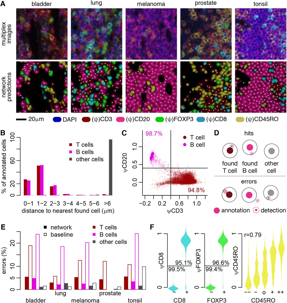
(A) Representative input images from 4 different types of tumor samples and a tonsillitis sample. (B) Distribution of distances between annotated cells and cells identified by the ImmuNet. (C) Expression of the CD3 and CD20 pseudomarkers (ψ) on detected cells. (D) Definition of correct and faulty detections used in (E), which shows the error rates of ImmuNet per tissue type compared to our baseline method. The detection radius used is 3.5 μm. (F) Distribution of pseudomarkers on detected cells compared to annotated marker expression on the nearest annotated cell. For CD8 and FOXP3, we grouped weakly and strongly positive or negative annotations.
Using a custom-built web browser-based data exploration and annotation tool, we annotated and decorated thousands of cells of various types and used this information to train our network and determine the parameters of the LoG filter (see Methods). Performance of our network typically did not improve anymore after about 100 epochs of training (taking 12-24 hours on our hardware), such that we were able to regularly visualize the output of our network and generate specific new training data in areas where we still detected problems during visual quality control. After several rounds of training, we had accumulated 36,856 cell annotations, could no longer find obvious problems with our network by visual inspection of the data, and were satisfied with the performance of the LoG postprocessing. We also trained baseline inForm segmentation and phenotyping algorithms on the same data, which unlike the ImmuNet approach required training a dedicated algorithm for each tissue type, and some-times multiple algorithms per tissue type if there were substantial differences between batches (such as changed microscope configuration settings).
After training our network and setting the LoG parameters, we measured the distance to the nearest detected cell for each annotated cell (Figure 3B). For the vast majority of annotated T- and B cells, ImmuNet detected a lymphocyte no further than 3μm away, which was almost never the case for non-lymphocyte annotations such as tumor cells or stromal cells. When we visualized the expression of CD3 and CD20 pseudomarkers on the nearest cells, they corresponded closely to the annotated phenotype. Specifically, for 96% of the annotated T cells and 99% of the B cells, the closest detected cell expressed the corresponding pseudomarker – but not the other pseudomarker – at an intensity of 0.4 or higher (Figure 3C). These findings suggested that the vast majority of the annotated cells were correctly detected by the final ImmuNet pipeline.
Given these results, we devised the following methodology to determine whether our cell detection pipeline was able to recover the cells it was trained on: for an annotated B- or T cell, we require the closest detected lymphocyte to be no further than 3.5μm away, and it must have the same phenotype as defined by pseudomarker cutoff of 0.4. For other annotated cells, no B- or T cell must be detected by the network within a 3.5μm radius (Figure 3D). Using this definition, we found the ImmuNet error rate to be consistently below 10% for annotated T cells, and below 5% for B cells and other cells (Figure 3E). For every possible combination of marker and tissue, comparing these values to the error rates of our baseline inForm algorithms (which were also trained on cell annotations collected from these datasets) suggested that our approach performed satisfactorily on the cell detection task.
We then determined whether the T cells in the training set that were correctly detected by ImmuNet also had the correct phenotype assigned. When annotating our cells, we generally found it easy to decide positivity for CD8 and FOXP3 markers, whereas the status of the CD45RO marker was more difficult to assess. We therefore grouped CD8 and FOXP3 cells into positive and negative. For these phenotypes, the network agreed with the annotator in at least 95% of the cases for both positive and negative cells (Figure 3F). For the more uncertain CD45RO marker, there was a more gradual correspondence between annotation and prediction, although the network agreed with the annotator in the vast majority of cases where the annotator was certain. Together, these results suggest that the ImmuNet pipeline is able to detect and phenotype immune cells in mIHC images based merely on sparse “click” annotations.
Having used our training data to set up our cell detection pipeline, train the neural network, and tune the parameters of the post-processing, we proceeded to evaluate the performance of our network on separately collected data that had not been used for network training and parameter tuning. For this validation dataset, we fully annotated the locations and phenotypes of all cells in small regions of interest (ROIs). While such annotations are substantially more difficult to collect than “sparse” annotations, they allow for a more robust investigation of our network’s performance; specifically, they enable analyses that penalize hypersegmentation of cells (i.e., splitting up a single cell into multiple detected cells). Ideally, the number of cells detected in each ROI should match the number of annotated cells in the same ROI. We indeed found this to be largely the case, although our baseline method sometimes substantially overestimated the number of cells in an ROI due to hypersegmentation (Figure 4A). Analyzing each tissue category separately, we found the agreement with our annotations to be consistently higher in the ImmuNet results than for our baseline method, sometimes by substantial margins (Figure 4B).

(A) Comparison of the number of cells detected within regions of interest (ROIs) at randomly chosen locations to manual lymphocyte counts within the same regions. (B) The data of (A) stratified by tissue type; error bars: 95% confidence intervals. Note that the X axis is chosen such that lower is better.
External validation of ImmuNet-determined phenotype abundance using flow cytometry measurements of the same tissue
Having found our ImmuNet results to perform satisfactorily compared to the baseline method, we next sought to validate our phenotyping results using external reference measurements. Flow cytometry is a mature and widely used non-spatial method for cell phenotyping. Because cells in a flow cytometer are dissociated and imaged one by one (rare duplicates can be filtered out in post-processing), and the entire outside of a cell is accessible to the cytometer, marker expression can be measured more reliably compared to mIHC imaging. We therefore decided to use flow cytometry as an external control for the relative lymphocyte phenotype abundances estimated by mIHC-based phenotyping. To this end, we obtained fresh human tonsillitis tissue. Tonsils contain extremely densely packed B- and T cell areas that are notoriously difficult to process for segmentation algorithms and therefore represented a useful test case for our analysis. For further processing, we split each tonsil in half (Figure 5A). One half of each tonsil was dissociated into single cells and analyzed by both flow cytometry and an FFPE AgarCyto cell block preparation [21] subjected to mIHC. The other half was directly FFPE and subjected to mIHC. We then used each of the three methods to quantify the amount of B cells, T cells, CD8+ T cells, FOXP3+ T cells, and CD45RO+ T cells as a proportion of all B- and T cells.

(A) Tonsils were cut in half with one half sliced and imaged by IHC, and the other half dissolved and further processed by flow cytometry or an AgarCyto preparation, which was also imaged by IHC. (B) Directly measured expression of CD3 and CD20 on segmented cells from the IHC images compared to the expression of the corresponding pseudomarkers on ImmuNet-detected cells. (C,D) Cells in AgarCyto (C) or direct FFPE (D) mIHC images were either phenotyped using the multiparametric classifier implemented in inForm (baseline), or using a threshold of 0.4 on the ImmuNet pseudomarkers (network). Concordance to flow cytometry (FCM) measurements from the same tonsils is shown and quantified using the intraclass correlation coefficient (icc), a measure of interrater agreement that ranges from 0 (no agreement) to 1 (perfect agreement).
Two-dimensional scatterplots of marker expression clearly showed distinct peaks representing T- and B cells for the flow cytometry data (Figure 5A). While two separate peaks were still somewhat apparent from the AgarCyto preparation analyzed with the baseline method, these disappeared when directly imaging the dense tonsil tissue (Figure 5B), resembling our initial findings on simulated data (Figure 1B). By contrast, separate peaks in the expression of ImmuNet pseudomarkers were still readily identifiable for both the AgarCyto preparation and direct tissue imaging (Figure 5B). To phenotype the cells based on their expression profiles, we again used the positivity threshold of 0.4 identified previously for CD3, CD8, FOXP3 and CD20 (Figure 3), and used a threshold of 0.25 for the more “gradual” CD45RO data. Given that a similar direct thresholding of expression markers would not seem sensible for the inForm data (Figure 5B), we instead trained and applied the inForm phenotyping classifier, which can take many additional features into account, to determine the baseline performance.
Reassuringly, our analysis showed good agreement between flow cytometry and mIHC measurements for the dissociated cells in our baseline analysis (ICC=0.89, 95%CI: 0.41-0.97) and in the ImmuNet data (ICC=0.97, 95%CI: 0.56-0.99; Figure 5C). The reason for the slightly worse baseline performance was an apparent systematic classification bias towards B cells, leading to a systematic underestimation of all T cell populations. However, when evaluating on the direct mIHC images, the agreement of the baseline method with flow cytometry data degraded substantially (ICC=0.64, 95%CI: 0.33-0.82), while the ImmuNet data still showed good overall agreement (ICC=0.89, 95%CI: 0.76-0.95).
An important caveat of this analysis is that one does not necessarily expect perfect agreement between flow cytometry and tissue images, because the spatial distribution of lymphocytes in the tonsil is not homogeneous. Because cells are dissolved for the AgarCyto preparation, the heterogeneity between different AgarCyto slides can be expected to be substantially less than the heterogeneity between FFPE slides from the tonsils, which should also lead to higher consistence between the AgarCyto and FCM data. Therefore, some of the higher disagreement observed in Figure 5D compared to Figure 5C can be due to spatial heterogeneity rather than segmentation or phenotyping errors. However, the better agreement of ImmuNet still suggests that a substantial part of the disagreement in the baseline method is indeed due to segmentation errors.
In summary, our external validation of mIHC phenotyping results by comparison to flow cytometry showed that the measurements obtained by both methods can be in good agreement provided that segmentation and phenotyping errors are sufficiently low. It appears that the improvements in cell phenotyping achieved by ImmuNet lead to better agreement with the more accurate (but non-spatial) flow cytometry data.
Discussion
We have developed, implemented, trained and tested ImmuNet, a machine learning pipeline for segmentation-free phenotyping of immune cells in mIHC imaging. Although relatively little information is used to train ImmuNet compared to segmentation-based machine learning architectures such as StarDist [10], we found it to perform well across diverse types of tissues, including very challenging dense environments. By design, ImmuNet is particularly well suited for applications where the cell shapes are not required for downstream analysis. This should often be the case for immune cells, because lymphocytes tend to lose their physiological shape in dead tissue and round up, such that there is little remaining meaningful variation. However, where this is not the case and the morphology of cells is important, one could combine ImmuNet with a cell segmentation of the same tissue. Indeed, the pseudo-marker profiles generated by the ImmuNet network could simply be added as additional channels to the image for further analysis in segmentation software such as CellProfiler [22] or ilastik [23]. Alternatively, a cell segmentation network like StarDist [10] could be extended with additional branches to generate ImmuNet pseudomarkers alongside segmentation maps.
The ImmuNet architecture shown in this paper is specifically trained for our T cell-focused antibody panel, but the procedure would work in the same way for other panels such as, for instance, our checkpoint molecule expression panel [2]. In practice, panels are adapted often, depending on the specific research question. A cautious approach would be to train a new ImmuNet from scratch for each panel. This would be laborious but it is feasible given the relative ease at which large numbers of annotations can be collected – using our internal tooling, we can typically annotate a few hundred cells per hour. However, when only one or two markers change, it may be effective to pool the data, especially if the alternative surface markers are of the same type (e.g., if one membrane marker is exchanged for another). Similarly, when some markers turn out to be unreliable in certain samples because of unspecific staining, one can still pool the data with other samples where the same marker is used but zero out the unreliable channel. In future research, we would like to investigate to what extent transfer learning strategies [24] could be employed to mix different channels in a more flexible manner. This may however not be straightforward for mIHC data given the spillover effects between adjacent channels frequently seen in such data, and might be a more fruitful avenue for other multiplex imaging techniques that are less affected by spillover such as CyTOF.
In summary, ImmuNet is a simple but effective machine learning pipeline for cell detection and phenotyping in multiplex imaging. Although we developed and tested ImmuNet for FFPE mIHC data, it should also be applicable to other multiplex imaging systems such as CyTOF, CODEX, and NanoString. We hope that ImmuNet pipelines will help researchers to generate more reliable phenotype maps of immune cells in tissue samples as a robust basis for diagnostic and prognostic applications of multiplex imaging technologies.
Materials and Methods
Simulation of artificial tissues
To generate synthetic in silico multiplex images, we used the cellular Potts model simulation framework. Cells were randomly placed in a 1283 μm3 volume and simulated at a resolution of 0.53 μm3 per voxel, matching resolution of real multiplex images. Cells consist of two compartments, a nucleus and a surounding cytoplasm region. Cells are randomly assigned a phenotype, with associated nuclear and membrane expressed markers matching real cells.
Simulation proceeds by placing seed voxels of cytoplasm for each cell at a random location, and lettting them circularize for 25 simulation steps. Then a nucleus seed voxel is placed inside each cell and the simulation is run for a further 50 steps so cells can settle into their final shape.
Settings controlling size of nucleus and cytoplasm per cell and adhesion strengths are described in Table 1. Simulation temperature was set at 20.
To simulate membrane expressed markers, all voxels on the outer layer of a cell’s cytoplasm compartment are found and marked as membrane. All voxels inside a cell’s nucleus are used for nuclear expressed markers. An 8 voxel slice is taken from the simulation volume, corresponding to a 4μm tissue slice, matching our imaged tumor tissue slides. For each simulated marker, expression is simulated in either membrane or nuclear voxels, and signals are integrated along the viewing direction to construct an image. An exact cell segmentation mask is extracted from simulation data from the middle of the 8 voxel thick slice.
Human material
Tonsils were collected from patients undergoing routine tonsillectomy at Canisius Wilhelmina Hospital in Ni-jmegen. Tonsils were stored at 4°C and processed within 24 hours. Tonsils were cut in halves of which one half was formalin fixed and paraffin embedded and the other half was processed into a single cell suspension. Fatty tissue was removed from the tonsil as much as possible with scalpels and placed into a gentleMACS C-tube (130-096-334, Miltenyi Biotec) with 5ml RPMI containing 0.3mg/ml Liberase (000000005401020001 Sigma) and 0.2mg/ml DNAse I (18068-015, Thermo Fisher). Tonsil tissue was roughly cut into smaller fragments using scissors and was further dissociated into a single cell suspension on the gentleMACS (130-096-334, Miltenyi Biotec) program “Multi_C_01_01” two times with a 15 minute incubation in between in a shaking water bath for 15 minutes at 37°C. 1 × 10⁶ cells were used for flow cytometry measurements and 1.5 × 10⁷ cells were fixed and embedded in paraffin with the AgarCyto cell block preparation [21].
From the Radboud university medical center (Radboudumc), melanoma specimens were randomly included based on the availability of a resection specimen. The study of the melanoma material collected at the Radboudumc was officially deemed exempt from medical ethical approval by the local Radboudumc Medical Ethical Committee concurrent with Dutch legislation, as we used leftover coded material and patients are given the opportunity to object to their leftover material to be used in (clinical) research.
The lung cancer samples were collected at the Netherlands Cancer Institute in the PEMBRO-RT Phase 2 Randomized Clinical Trial [25] approved by the institutional review board or independent ethics committee of the Netherlands Cancer Institute–Antoni van Leeuwenhoek Hospital, Amsterdam. All lung cancer patients provided written informed consent and consented to further analysis of patient material collected prior to and during the PEMBRO-RT trial.
The bladder cancer samples are derived from patients who were treated for metastatic bladder cancer at the Rad-boudumc between 2016 and 2019. Archival tissue of both primary and metastatic tumor lesions was used. Prostate cancer samples are derived from patients that were treated in the Radboudumc and include archival tissue of both primary and metastatic tumor lesions. The research on prostate and bladder cancer samples was approved by the local Radboudumc Medical Ethical Committee (file number 2017-3934). All patients provided written informed consent to scientific use of archival tissue, unless deceased.
Flow cytometry
Single cells from tonsil (106) were stained with Fixable Viability Dye eFluor™ 780 (eBioscience, 65-0865-18, 1:1000) for 20 minutes at 4°C. After wash steps, cells were incubated with a mix of anti-CD3-BV421 (BD Bio-science, 563798, clone SK7, 1:25), anti-CD8-PerCp (BD Bioscience, 345774, clone SK1, 1:5), anti-CD45RO-APC (BD Bioscience, 340438, clone UCHL-1, 1:25), and anti-CD20-PE (Biolegend, 302306, clone 2H7, 1:10) for 30 minutes at 4°C. Next cells were fixed, permeabilized with Foxp3/Transcription Factor Staining Buffer Set (eBio-science, 00-5523-00) and incubated with anti-FOXP3-alexa488 (eBioscience, 53-4776-42, clone PCH101, 1:8) 30 minutes at RT. Flow Cytometry was conducted with the FACS Verse (BD Biosciences). Flow cytometry data was analyzed using FlowJo software (v10, Tree Star).
Multiplex immunohistochemistry staining
Sections of 1-4 μm thickness were cut from FFPE tissue blocks containing tonsil, melanoma and AgarCyto preparations respectively. The slides were subjected to sequential staining cycles as described before [2], although now automated using Opal 7-color Automation IHC Kit (NEL801001KT; PerkinElmer) on the BOND RX IHC & ISH Research Platform (Leica Biosystems) as described previously [26]. All heat induced epitope retrievals were performed with Bond™ Epitope Retrieval 2 (AR9640, Leica Biosystems) for 20 minutes at 95°C. Blocking was performed with antibody diluent. Primary antibody incubations were performed for 1 hour at RT. All secondary antibody incubations were performed for 30 minutes at RT. mIHC was performed with anti-CD45RO (Thermo Scientific, MS-112, clone UCHL-1, 1:3000) and Opal620, anti-CD8 (Dako, M7103, clone C8/144B, 1:1600) and Opal690, anti-CD20 (ThermoFisher, MS-340, clone L26, 1:600) and Opal570, anti-CD3 (ThermoFisher, RM-9107, clone RM-9107, 1:400) and Opal520, FOXP3 (eBioscience Affymetrix, 14-4777, clone 236A/E7, 1:300) and Opal540. For prostate cancer samples, anti-CD56 (Cell Marque, 156R-94, clone MRQ-42, 1:500) was used with Opal570 instead of anti-CD20.
To visualize tumor cells, melanoma tissues were stained in the end with a melanoma mix consisting of anti-HMB-45 (Cell Marque, 282M-9, clone HMB-45, 1:600), anti-Mart-1 (Cell Marque, 281M-8, clone A103, 1:300), anti-Tyrosinase (Cell Marque, 344M-9, clone T311, 1:200) and anti-SOX-10 (Cell Marque, 383R-1, clone EP268, 1:5000) and Opal650 to visualize tumor tissue. Tonsil, bladder and lung cancer tissues were finished with anti-pan cytokeratin (Abcam, ab86734, clone AE1/AE3 + 5D3, 1:1500) and Opal650 to visualize epithelial tissue. Finally, epithelial tissue in prostate cancer samples was visualized with a mix consisting of anti-pan cytokeratin (Abcam, ab86734, clone AE1/AE3 + 5D3, 1:1500), anti-EPCAM (Abcam, ab187372, clone VU-1D9, 1:1000) and anti-PSMA (Bio SB, BSB6349, clone EP192, 1:1000) and Opal650. Slides were counterstained with DAPI and mounted with Fluoromount-G (SouthernBiotech, 0100-01).
Tissue imaging and data preparation
Slides were scanned using the PerkinElmer Vectra 3.0.4. Multispectral images were unmixed using spectral libraries build from images of single stained tissues for each reagent and unstained tissue using the inForm Advanced Image Analysis software (inForm 2.4.1, PerkinElmer). A selection of 15 to 25 representative original multispec-tral images were used to train the inForm software (tissue segmentation, cell segmentation, phenotyping tool and positivity score). All the settings applied to the training images were saved within an algorithm allowing batch analysis of multiple original multispectral images of the same tumor.
Artificial neural network
Rationale for network architecture choices
Analysis of cellular images has greatly advanced in recent years with the introduction of deep learning algorithms [27]. Using these algorithms, cell segmentation can be formulated as a pixel-wise supervised learning task, where e.g. each pixel is classified as being part of a cell, a cell boundary or as background. Fully convolutional neural networks (FCNNs) are one method to perform pixel classification on whole images [28]. For each pixel the FCNN gets to see a “receptive field” of surrounding pixels, allowing it to use local context to judge cell type and boundary shape per pixel. An important variant of this approach is U-Net [29]. U-Net is designed for whole slide analysis; where FCNNs only see smaller structures in an image, U-net integrates both pixel level detail and large scale information to segment structures bigger than an FCNN can perceive.
We had initially compared FCNN and U-net architectures, and in early testing they performed comparably. We found the FCNN architecture a more natural fit for our sparse annotations, and hypothesized that because we segment cells that are small enough for an FCNN to observe, our task might not benefit greatly from U-Net’s ability to take larger environments into account. For these reasons, we decided to use an FCNN architecture, but we are planning to explore how this compares to U-net on our current data in future research.
In the early stages of our development process, we had considered and compared both location-based and cell shape-based annotations, taking the idea for location annotations from earlier studies on IHC data that used fully annotated training images [30,31]. During our early testing we found location-based annotations combined with a distance transformation to perform well, and therefore did not proceed with the much harder to obtain shape-based annotations. We experimented with splitting up distance and phenotype predictions in separate FCNNs, or have dedicated networks for B and T cells; however, in the end we found that single networks combining distance and phenotype predictions performed reasonably and were easier to use. In our testing, enlarging the output map of the FCNN from 1×1 to 3×3 pixels and adding ResNet-inspired skip connection appeared to be beneficial.
In summary, the final backbone of our system is a prediction of distance to cell center, which is designed for ease of annotation and post-processing (i.e. for a peak-finding algorithm), and reasonably approximates the shape of many lymphocytes, which are often round.
Network training, cell detection, and implementation
We used an Adam optimizer [32] during training with a learning rate of 0.001, and mean squared error loss functions for both phenotype and distance pixel map predictions. Different weights were assigned to phenotype and distance map losses: 20 and 1 respectively. Phenotype loss functions could easily be replaced with categorical cross-entropy when binary predictions are desired, but this allowed us to both train on biologically more gradual markers like CD45RO, and include our Likert scale annotations in training. We normalize each channel per tile by using the default percentile-based normalization from the CSBdeep python library [33]. During training we add Gaussian noise with a standard deviation of 0.1 to input and apply random data augmentations. Specifically, we perform horizontal and vertical flips and rotations, and change the input image intensities randomly in the same way as StarDist [10] by first multiplying the input with a uniformly distributed scalar s1 ~ U(0.6, 2) and then adding another uniformly distributed scalar s2 ~ U(−0.2, 0.2). Convolutional layers perform batch normalization during training; fully connected layers perform dropout with a rate of 0.2.
We predict a circle with a radius of 5 pixels (2.5 μm) around each annotated lymphocyte, with a value of 5 at the center, that drops to a value of 0 at the border of the circle. For pixels not part of annotated cells, we set the distance transform to −2. For each phenotype pseudomarker, the 5-point Likert scale is mapped to the values 0,0.25,…,1.
To detect and phenotype cells based on the distance and pseudomarker predictions of the network, we first post-process the distance pixel map prediction with a Laplacian-of-Gaussian filter as implemented in scikit-image [34], using parameters min_sigma=3, max_sigma=5, and threshold=0.07. Then, for each detected cell location and each pseudomarker channel, we determined the mean expression value of that channel within a radius of 2 pixels around the center, and used this as the pseudomarker expression vaulue of the cell.
The final network used in this paper was trained on 231851 63×63×6 input environments taken from 36856 cells. Training was run for 76 epochs, which took 12 hours. Neural networks were constructed with TensorFlow [35], with important post-processing done in NumPy [36], SciPy [37] and scikit-image [34]. Source code along is available at https://github.com/jtextor/immunet. Images and annotations for the AgarCyto data will be deposited on Zenodo and will be linked to from the GitHub page.
Acknowledgements
We thank Dr. Willem Vreuls and Dr. Roland Pennings for providing tonsil tissues.
JT and SS were supported by the Dutch Cancer Society - Alpe d’HuZes foundation (grant 10620). JT and FB were supported by NWO grant VI.Vidi.192.084. MG, LvdW, KV, and CF were supported by Dutch Cancer Society grants 10673 and 2017-8244. CF was also supported by a grant from Oncode Institute and by ERC advanced grant ARTimmune 834618. EM was supported by a grant from the Hanarth Fonds (to JT).
References


