

Abstract
Our ability to flexibly adapt to changing demands is supported by flexible coding of task-relevant information in frontal and parietal brain regions. Converging evidence suggest that coding of stimuli and task rules in these regions become stronger as task difficulty increases. Here, we tested whether there is a corresponding change in the representational format as well, an issue that has rarely been addressed directly in past research. Participants performed a visual classification task under varying levels of perceptual difficulty, while we acquired fMRI. Using a model-based representational similarity approach, we tested whether stimulus representations retain exemplar-level information. We expected representations to drop such exemplar-level information as perceptual difficulty increases, which would indicate a focus on representing behaviorally relevant category information. Counter to these expectations, and in contrast to previous research, we found frontal and parietal brain regions contained exemplar-level stimulus information. Interestingly, the anterior intraparietal sulcus (aIPS) retained exemplar-level stimulus information even in perceptually difficult trials, and these representations were directly related to performance. Overall, these findings call for a reassessment of the neural mechanisms underlying human adaptive behavior during visual classification.
1. Introduction
Humans are able to rapidly, flexibly adapt to changing external demands (Fuster, 2000; Miller, 2000). Regardless of the current context in which we find ourselves, we can efficiently adjust our behavior to current demands, an ability that is supported by frontal and parietal brain regions often called the multiple demand (MD) network (Duncan, 2010; Fedorenko et al., 2013). We know from past research using multivariate decoding (Haynes, 2015; Kamitani & Tong, 2006) that MD regions encode a wide range of task-related information, including stimuli, responses, and task-rules (Woolgar et al., 2016), with preferential coding of task features that are task-relevant or explicitly attended (Jackson et al., 2017; Jackson & Woolgar, 2018; Woolgar, Williams, et al., 2015). Coding of task-related information in these regions is also especially strong when tasks are difficult (Woolgar, Hampshire, et al., 2011; Woolgar, Afshar, et al., 2015) and specifically affected when part of the MD system is modulated with TMS (Jackson et al., 2021). This has been taken as evidence for adaptive coding (Duncan, 2010), in which multi-modal neurons flexibly change their coding properties to meet current, changing demands. Adaptive coding in these regions is thought to be a key mechanism underlying selective attention (Duncan, 2013), providing a source of bias over coding in sensory and motor brain regions (Desimone & Duncan, 1995). Additional evidence for adaptive coding comes from fMRI studies showing that coding of task-related information changes across reward-conditions (Etzel et al., 2016) and free vs cued task choices (Zhang et al., 2013), and MEG studies showing rapid prioritization of task-relevant information processing (Barnes et al., 2021; Goddard et al., 2019; Moerel et al., 2021). On the other hand, we know that at least under some conditions, frontoparietal representations of task-related information does not adapt to changing demands (Loose et al., 2017; Wisniewski et al., 2016, 2019). For example, it has been suggested that MD cortex might be better able to adjust to cope with changes in conceptual difficulty than changes in the quality of perceptual input (Wen et al., 2018), although apparently compensatory increase in coding following poor perceptual input has also been observed (Woolgar, Thompson, et al., 2011; Woolgar, Williams, et al., 2015). Thus it remains an open question whether adaptive coding is a general property of these regions, or whether frontoparietal cortex only adapts its representations under specific circumstances, and instead re-uses the same representations when necessary (Botvinick & Cohen, 2014; Feng et al., 2014; Wisniewski, 2018).
In addition, while previous research attempted to answer whether coding adapts to different task demands, it did not address the issue of how coding might differ across demands, which would require testing whether a set of representational models explain the data. For example, previous studies have asked whether information coding is stronger in hard than in easy trials (Woolgar, Hampshire, et al., 2011), and, using cross-classification (Kaplan et al., 2015), whether coding formats are similar or different across conditions (Wisniewski et al., 2016; Zhang et al., 2013). These studies have been optimized to test for the presence or absence of a difference in representations across conditions (whether), but make no explicit predictions about the nature of that difference (how). Showing that coding is stronger in hard trials might be explained by the strengthening of the same representation, or by a change in the representational format used. Thus, it remains difficult to draw strong conclusions about specific representational formats used in different conditions, and about how these formats change. Here, we argue that understanding adaptive coding at the level of representational formats is key to understanding the neural basis of goal-directed attention and its biasing influence on sensory and motor processing.
In the current study, we directly addressed this issue by designing a task that allows us to investigate the representational formats used to encode task-related information in MD regions in hard and easy trials, and to quantify how these formats changed across difficulty conditions. For this purpose, we combine a visual categorization task (Freedman et al., 2003) with representational similarity analysis (RSA) of fMRI data (Kriegeskorte, Mur, & Bandettini, 2008; Nili et al., 2014), which offers a powerful tool to formulate specific hypotheses about how representational formats change across easy and hard trials.
Participants performed a simple classification task, determining whether visual stimuli are either cats or dogs. Difficulty was manipulated by morphing cat and dog stimuli (morph level, ranging from 100% cat to 100% dog stimuli), and by adding random Gaussian noise to the images (noise level, clean vs noisy stimuli). We expected MD regions to encode visual stimulus and category information, as has been shown before in tasks with similar designs (Jackson et al., 2017, 2021; Jackson & Woolgar, 2018). Crucially, we tested in which format stimulus information was encoded, and whether this changed when we manipulated perceptual difficulty (noise level). Neural representations could either preserve stimulus distances of individual exemplars in physical space (isomorphic coding, which we call ‘equidistant’ coding here since stimuli were equidistant in physical space). Alternatively, neural representations could cluster stimulus representations of individual exemplars belonging to the same category, with neural distances being small within categories and large between categories (see Figure 1A). Equidistant coding essentially preserves exemplar information, representing the full perceptual space, including differences between individual dog (or cat) exemplars that are irrelevant to the categorization task. Clustered coding collapses representations of individual exemplars and emphasizes differences between the two categories, and is thus optimized for performance in this task. These two different coding formats would be indistinguishable using the design and analysis methods from past research, since multivariate decoding could differentiate the two categories of stimuli regardless of whether representations are equidistant or clustered. Past research in non-human primates has suggested that sensory regions show veridical equidistant coding, whereas dorsolateral prefrontal cortex (dlPFC) shows clustered coding (Freedman et al., 2003). Furthermore, object-selective regions in the ventral visual stream preserve information about specific exemplars within a category (Eger et al., 2008).

A. Stimuli. On the left, all template images used here are depicted. All stimuli above the decision boundary are cats, all below are dogs. Each participant was presented 2 out of 3 cat/dog templates (randomly selected for each participant). In the middle, example morphed stimuli are depicted for 2 dog and 2 cat template images. On the right, a schematic representation of clustered and equidistant coding is depicted. When stimulus representations are clustered, representational distances between exemplars of the same category (e.g. dog) are small, i.e. representations are highly similar. Distances between categories are large. When stimulus representations are equidistant, distances from the perceptual space (middle) are preserved in the neural space, including differences between exemplars within the same category. B. Trial timing. Each block started with an instruction screen. Then, stimuli were presented for 1.8s, interleaved with a variable inter-trial-interval (mean duration 2.7s, range 0.8 – 10.4s).
We hypothesized that clustered coding should be especially useful when task difficulty is high, i.e. when there is a clear need to optimize neural representations to improve performance. This prediction is derived from recent theories, which argue that task representations vary from low to high-dimensional (Badre et al., 2021; Botvinick & Cohen, 2014), and that this difference is related to a trade-off between pattern separability and generalizability. High-dimensional representations, like those preserving exemplar-level information in our design (equidistant coding), allow for better separation of individual stimuli, but are harder to generalize to novel contexts and are more susceptible to noise (Fusi et al., 2016). Low-dimensional representations, like those collapsing to just a single relevant stimulus dimension in our design (clustered coding), are harder to separate, but are more easily generalized to novel contexts and are less susceptible to noise. Therefore, we expected a shift towards more clustered coding on perceptually difficult trials, reasoning that this change in representational formats is a key neural mechanism of how MD regions adapt to changing task demands.
In sum, we expected that visual regions would encode stimuli using an equidistant format on trials in which stimuli can be clearly seen (clean trials), and that this signal might be weaker or absent on trials in which stimuli are noisy (Hypothesis 1). For MD regions we expected a different pattern of results. Past research has shown that MD regions represent task-related information like object categories preferentially in difficult trials (Woolgar, Hampshire, et al., 2011; Woolgar, Williams, et al., 2015), and we thus expected stimulus coding to be weaker on clean than on noisy trials (Hypothesis 2). If we found stimulus information on clean trials, we expected it to be in an equidistant format, reflecting bottom-up information from sensory regions that should be sufficient to correctly classify stimuli. On noisy trials, we further expected a shift from equidistant to more clustered coding (Hypothesis 3), based on previous theories (Badre et al., 2021; Botvinick & Cohen, 2014). Such a shift in representational formats might be a key neural mechanism of how MD regions adapt to changing task demands.
2. Methods
2.1 Participants
Forty-nine volunteers (38 female, 11 male, mean age: 24.1 years, range: 18-36 years) with normal or corrected-to-normal vision participated in the study. We obtained written informed consent from each participant prior to participation, and the Ethics Committee of the Ghent University Hospital approved this experiment (project identifier BC-07446). Each volunteer received 43€ for their participation. We first calculated the average error rate for each participant in the easiest possible condition in this experiment (clean template images, see below for more details). Five participants had excessive error rates (above 1.5*IQR of the group mean,): 10.4%, 10.4%, 12.5%, 16.7%, and 22.9% respectively, group average = 3.1%. These participants were excluded from the sample. Four participants showed excessive head movement during scanning (> 5mm), and were also removed. Two additional subjects were removed due to technical difficulties. The final sample consisted of thirty-eight participants (29 female, 9 male, mean age = 24.4 years, range: 19-36 years).
2.2 Task and Experimental Paradigm
On each trial, participants performed a perceptual classification task, determining whether a visual stimulus presented centrally on screen was a cat or a dog. The stimulus was a morphed image, ranging from 100% dog to 100% cat, and could be presented in one of two different perceptual difficulty levels (clean and noisy).
2.2.3 Stimuli and Design
Stimuli consisted of a large set of gradually, smoothly morphed, greyscale stimuli, created using 3 cat templates to 3 dog templates (Fig. 1A), two of which were used for each participant (see below). Stimuli were created by linearly combining one cat and one dog template, with changing contributions (morph level, e.g. 93.4% cat, 6.6% dog, with steps of 6.6%). These stimuli have been used before on non-human primate research, and for more detail on their generation please see (McKee et al., 2014). For each combination of cat and dog templates, 16 stimuli were created (1 dog template + 1 cat template + 14 morphed stimuli). Given that there were 9 different template combinations (between 3 cat and 3 dog templates), the full stimulus set consisted of 144 stimuli. Each stimulus was categorized as either cat or dog depending on which category contributed more to the image (>50%). This yielded 72 cat and 72 dog stimuli, which differed in their distance to the category or decision boundary (choice difficulty). We then used these images, and added random Gaussian noise to them, in order to make the classification more difficult (noise level). The amount of added noise was adapted to each participant using a staircase procedure (see below).
For each participant, we randomly selected 2 dog and 2 cat template images, and used all four possible template combinations between cats and dogs as stimuli. We morphed each cat and dog template combination (cat1 – dog 1, cat 1 – dog 2, cat 2 – dog 1, cat 2 – dog 2) in 16 steps (ranging from 100% cat to 100% dog). This yielded 8 dog stimuli and 8 cat stimuli for each template combination. For both dogs and cats, the 8 stimuli differed in their choice difficulty, i.e. distance to the decision boundary, in 8 steps (e.g. 100% dog, 93.3% dog, 86.7% dog, 80% dog, 73.3% dog, 66.7% dog, 60.4% dog, 53.4% dog). Additionally, each of these stimuli was presented with a low noise level (clean) and a high noise level (noisy), resulting in a 2 (categories) x 8 (choice difficulties) x 2 (noise levels) x 4 (template combinations) design with 128 unique stimuli.
2.2.5 Procedure
The experiment was programmed using PsychoPy3 (v.2020.1.3, (Peirce, 2007)). Participants started by performing a short training session outside the MR scanner. During the training session, participants received trial-by-trial feedback on their responses. They first learned to classify template images, followed by classifying noise-free morphed images (clean trials). They then entered the MR scanner, where they completed a staircase procedure to calibrate the noise level in the scanning environment for each individual. For this purpose, we presented template stimuli with varying levels of noise added. After each correct response, random Gaussian noise increased. After each wrong response, noise decreased. We then counted how often the direction of noise level changes reversed (increase then decrease, decrease then increase). After 7 reversals, the staircase procedure stopped and we applied the final noise level to all noisy stimuli used in the experiment.
After that, participants performed 6 runs of 128 trials of the experimental task. In each trial, a stimulus was presented on screen for 1.8 sec (Figure 1B), which was followed by a variable, pseudo-exponentially distributed inter-trial-interval (ITI, mean duration = 2.7 sec, range between 0.8 sec to 10.4 sec). Participants were instructed to respond while the stimulus was presented on screen, as quickly and accurately as possible. As an additional incentive, any participant that was both in the top 20% fastest and the top 20% most accurate participants would receive a 10€ bonus payment. Note that being either fast or accurate was not enough, the bonus payment required speed and accuracy. Participants responded using the left and right index fingers, using MR-compatible response boxes. Category-button-mappings were counter-balanced across runs for each participant (dog: right, cat: left in half of the runs, dog: left, cat: right in the other half). Participants received feedback at the end of each run (mean error rate + mean reaction time).
In each run, each unique stimulus was presented once, resulting in 4 repetitions of each combination of category, choice difficulty, and noise level. In order to increase the signal-to-noise ratio in the fMRI data, we collapsed the 8 levels of choice difficulty to just 4 for the analysis, doubling the number of repetitions to 8 per run. Category, choice difficulty, and template combination were pseudo-randomized and changed on a trial-by-trial basis. Noise level was blocked, and each run consisted of 4 blocks of 32 trials each. Two blocks were noisy, two blocks were clean, and half of the runs started with a noisy block, while the other half started with a clean block. Each block started with an instructions screen presented for 5 sec (‘Easy block starting now’, ’Hard block starting now’). To ensure that none of the design variables were correlated after randomization, we computed the mutual information between each design variable within each run separately. Only if there was no mutual information between any design variable (tested using permutation tests, p > 0.05), did we use the design in the experiment. We used the same procedure to ensure that there were no sequential dependencies between trials, so that conditions on trial t were unrelated to conditions on trial t+1.
Due to a coding error, for the first 29 participants, the 6 runs contained different numbers of cat and dog stimuli for each combination of choice difficulty and noise level. This introduced additional noise to the data, and made signal estimation in some conditions and some runs more difficult. However, due to the mutual information test we employed before accepting designs, we ensured that this did not introduce any systematic biases even within participants.
2.3 Image acquisition
Functional imaging was performed on a 3T Siemens Prisma MRI scanner (Siemens Medical Systems, Erlangen, Germany), using a 64-channel head coil. For each of the six functional scanning runs, we acquired 350 T2*-weighted whole-brain echo-planar images (EPI, TR = 1730 ms, TE = 30 ms, image matrix = 84 × 84, FOV = 210 mm, flip angle=66°, slice thickness = 2.5 mm, voxel size = 2.5 × 2.5 × 2.5 mm, distance factor=0%, 50 slices with slice acceleration factor 2). Slices were oriented along the AC-PC line for each participant. A T1-weighted structural scan was acquired prior to the functional scans (MPRAGE, TR = 2250 ms, TE = 4.18 ms, TI = 900 ms, acquisition matrix = 256 × 256, FOV = 256 mm, flip angle=9°, voxel size = 1 × 1 × 1 mm). We further acquired 2 field maps (phase and magnitude) to correct for inhomogeneities in the magnetic field (TR = 520 ms, TE1 = 4.92 ms, TE2 = 7.38 ms, image matrix = 70 × 70, FOV = 210 mm, flip angle=60°, slice thickness = 3 mm, voxel size = 3 × 3 × 2.5 mm, distance factor=0%, 50 slices).
2.4 Analysis: Behavior
Behavioral data were analyzed using RStudio (version 1.2.1335, R version 4.0.3). We first removed all trials on which the participant failed to respond. On average, we removed 1.66% (SD = 0.64%) of all trials for each participant this way. Additionally, we removed trials with RTs < 150ms, removing 1.68% of trials on average (SD = 0.64%). To assess task performance, we extracted mean RTs and error rates for each combination of noise level and choice difficulty. For the RT analysis, we only used correct responses. RTs were then entered into a Bayesian ANOVA (BayesFactor::anovaBF, using the default scaled inverse chi-square prior on main effects and interactions, scaling factor fixed effects = 0.5, scaling factor random effects = 1), testing for evidence for or against both main effects and their interaction. Participants were entered as a random effect into this model. We interpreted the resulting Bayes Factors (BF10) according to the following guidelines (Wagenmakers, 2007): BF10 between 1 and 3 are interpreted as anecdotal, between 3 and 20 as moderate, between 20 and 150 as strong, and >150 as very strong evidence for the alternative hypothesis. BF10 between 0.33 and 1 are interpreted as anecdotal, between 0.05 and 0.33 as moderate, between 0.007 and 0.05 as strong, and <0.007 as very strong evidence for the null hypothesis. The same procedure was then applied to error rates.
In order to characterize performance better, we additionally fitted psychometric functions to the choice data, separately for each participant (Weibull function, quickpsy package, (Linares & López-Moliner, 2016)). Specifically, we computed the probability of choosing the dog response separately for each combination of morph level and noise level, and then fitted psychometric functions separately for both noise levels. This allowed us to extract several key parameters from the choice data: k, guess rate, and threshold. k determines the slope of the psychometric function and describes how sharply both categories are distinguished. The guess rate quantifies how often participants guess, and we expected k to be lower and the guess rate to be higher on noisy, as compared to clean, trials. To test this hypothesis, we entered estimates into a Bayesian paired t-test (BayesFactor::ttestBF, Cauchy prior, scaling factor = 0.707), comparing parameter values across noise levels. The threshold quantifies at which point on the scale of morphed images, ranging from 100% cat to 100% dog, participants were equally likely to choose cat or dog. We expected this to fall in the middle of the scale, i.e. where stimuli are close to 50% cat / 50% dog, and tested this hypothesis using a Bayesian t-test (Cauchy prior, scaling factor = 0.707).
2.5 Analysis: fMRI
fMRI analyses were performed using Matlab (R2018b, version 9.5.0.944444, The Mathworks), SPM12 (https://www.fil.ion.ucl.ac.uk/spm/), The Decoding Toolbox (v 3.99, (Hebart et al., 2014)), and RStudio (version 1.2.1335, R version 4.0.3). Raw data were first unwarped, realigned, and slice-time corrected (code: https://github.com/CCN-github/fMRI-preprocessing-SPM12). We then estimated normalization fields for each participant, which were then used to project mask files from normalized to native space (see below for more details). However, no spatial smoothing or normalization were applied to BOLD data to preserve fine-grained voxel activation patterns.
2.5.1 First-level GLM analysis
The preprocessed data were used to estimate a voxelwise general linear model (GLM, (Friston et al., 1994). Sixteen regressors of interest were used, one for each combination of category (cat, dog), noise level (clean, noisy), and choice difficulty (1,2,3,4). We then added a variable number of nuisance regressors for each participant. First, we added condition-specific error regressors, modelling error trials separately for each condition. This led to a variable number of nuisance regressors, since not every run had errors in each condition. We chose condition-specific error regressors over a single error regressor, since we expected errors in very easy trials to derive from different processes than in very difficult trials. For example, errors in easy trials might represent a momentary lapse in attentional or motor processes, while errors in hard trials likely represent guessing in the face of little available stimulus information. Second, we added six movement regressors. Regression was time locked to the onset of the stimulus presentation. As a base function, we used the finite impulse response function (FIR, 5 time bins with a duration of 1.73 sec each). In contrast to the canonical haemodynamic response function, FIR functions make fewer assumptions about the shape of the haemodynamic response, making it better suited to model responses to short events in a heterogeneous set of brain regions from visual to prefrontal cortex (see Wisniewski et al., 2015 for a similar approach).
2.5.2 Feature selection
ROI selection
We defined a number of a-priori volumetric regions-of-interest (ROIs), based on a recent publication outlining the multiple demand (MD) network using the Human Connectome Project atlas (Assem et al., 2020). The following regions were included in this experiment: SCEF, 8BM, 8C, IFJp, p9_46v, a9_46v, i68, AVI, IP1, IP2, PFm (see Figure 2, code: https://github.com/davidwisniewski/fmri-extract-HCP-mask). As an additional region of interest, we used the ventral visual cortex, as defined using the Harvard-Oxford atlas. Data from the chosen ROIs was extracted in native space for each subject, by projecting the ROI masks from MNI to native space separately for each participant, using the inverse normalization field estimated during pre-processing.

ROIs were derived from the HCP atlas (Glasser et al., 2016), and included the multiple demand regions identified in (Assem et al., 2020). The ventral visual cortex ROI was defined using the Harvard-Oxford atlas.
Time-bin selection
Given that we use the FIR basis function, each regressor is modelled at five different time points. To select a time window of interest, we first estimated the haemodynamic lag to be 2TRs (3.46 sec), based on previous research using MVPA methods to extract task-related information from fronto-parietal cortex (Bode & Haynes, 2009; Momennejad & Haynes, 2013; Wisniewski et al., 2015). We then corrected for haemodynamic lag by using data from time bins 3 and 4, which started 3.46 sec and 5.19 sec after stimulus onset, respectively, for all multivariate pattern analyses. Again, this follows past research on time-resolved pattern analysis of task-related information (Momennejad & Haynes, 2012). We expected haemodynamic responses to be short, given that the trial duration / stimulus processing was short, and this procedure strikes a balance between accounting for the expected short duration, and still allowing for the peak response to occur within a variable time window (between 3.46 sec and 6.92 sec after stimulus onset).
2.5.3 Representational similarity analysis
For each ROI, we first extracted the beta weights for the 16 regressors of interest in each run (2 categories x 2 noise levels x 4 choice difficulty levels). We then used The Decoding Toolbox (Hebart et al., 2014) to perform a representational similarity analysis (RSA, (Kriegeskorte, Mur, & Bandettini, 2008; Nili et al., 2014), using the cross-validated Euclidean distance measure and applying multivariate noise normalization (Walther et al., 2016). For this, we split the dataset into two independent parts by leaving a single run out in each fold of the cross-validation procedure. We then computer pairwise Euclidean distances between each pair of conditions, across the two parts. We repeated this procedure until each run had been left out once, leading to a six-fold cross-validation, and then averaged distances across folds. Using cross-validated distances ensures that estimates are unbiased and average to zero if there is no systematic relation between activation patterns (Arbuckle et al., 2019). All computed distances were then converted to a 16×16 representational distance matrix (RDM), representing pairwise distances between all conditions. This procedure was performed separately for each ROI, and for each of the two time bins of interest. For each ROI, we then averaged the RDMs across both time bins.
2.5.4. Model-based RSA
The main goal of this experiment was to identify whether and how stimulus information is encoded in the MD network. For this purpose, we first defined two alternative theoretical models of how stimulus information could be encoded in the brain.
First, stimulus information can be encoded in an equidistant format, i.e. all distances in the perceptual space can have an equivalent representation in neural representational space (Figure 3). Here, the full perceptual space is preserved in neural space, e.g. if a stimulus is 6.6% more ‘doggy’ than another stimulus, that distance will be half as large as to a stimulus that is 13.2% more ‘doggy’ in neural state space, irrespective of whether the two compared stimuli cross the decision boundary or not. This model assumes that slight perceptual differences between individual cat (and dog) stimuli are preserved, despite not being relevant for in the categorization task whatsoever.

On the left, an example data representational distance matrix (RDM) is depicted, from the anterior intraparietal sulcus (IP2). Each of the 16 conditions (2 categories: cat, dog; 4 choice difficulty levels: cd1, cd2, cd3, cd4; 2 noise levels: clean, noisy) is represented in one row / column. Each cell represents the pairwise cross-validated Euclidean distance (cvDistance) between beta vectors from the corresponding conditions. Dark colors indicate low distances, while bright colors indicate high distances. In the middle, two stimulus coding models are represented in the same RDM format as the data. On the right, a schematic representation of our partial correlation analysis demonstrates how unique shared variance between each model and the data RDM was computed.
Second, stimulus information can be encoded in a clustered, i.e. all distances between individual stimuli within a category (all dogs or all cats) are very small, while distances between categories are large. Here, coding of slight perceptual distances between individual stimuli within a category is dropped, and only the behaviorally relevant feature of the stimulus (category) is encoded.
2.5.5 Zero-order correlations
In order to test whether visual and/or fronto-parietal regions encode stimulus information, we first computed canonical, zero-order Spearman correlations between the two models and the data, separately for each participant. For this purpose, we only considered data from the lower half of the RDM, excluding the diagonal. These correlations were Fisher-z transformed and entered into a Bayesian one-sided t-test (BayesFactor::ttestBF, Cauchy prior, scaling factor = 0.707) to assess whether they were above zero. This analysis was performed for each ROI separately, and only using data from clean trials since stimulus information should be strongest here. Note that in principle, model-based RSA allows us to independently investigate evidence for both models, i.e. both, only one, or no model could potentially explain the data. Thus, even if both models partly explained the data, we would be able to identify this pattern of results.
2.5.6 Hypothesis 1: Visual cortex uses an equidistant coding format
We hypothesized that stimulus information in ventral visual cortex is represented in an equidistant format on clean trials. While the manipulation check assessed whether either model explains variance in the data, zero-order correlations do not control for potential correlations between the two explanatory variables / models. Given that the clustered and equidistant coding models correlated positively with one another (r = 0.66), we used partial Spearman correlations to investigate unique shared variance between the equidistant coding model and data RDMs extracted from visual cortex, while controlling for shared variance with the clustered coding model. This analysis was performed separately for clean and noisy trials, again only using the lower half of the RDM and excluding the diagonal. Partial correlation coefficients were then Fisher-z transformed and entered into a Bayesian one-sided t-test (BayesFactor::ttestBF, Cauchy prior, scaling factor = 0.707) to assess whether the partial correlation was above zero. To directly test whether equidistant coding became weaker on noisy trials, we computed paired Bayesian one-sided t-tests (BayesFactor::ttestBF, Cauchy prior, scaling factor = 0.707) between clean and noisy trials, expecting correlations to be weaker on noisy trials.
As a control analysis, we computed the opposite partial correlations, between the clustered coding model and data, controlling for any shared variance with the equidistant coding model. We did not expect to see evidence for positive correlations in this analysis in the visual cortex.
2.5.6 Hypothesis 2: Weak stimulus coding on clean trials in MD regions
For clean trials, we expected to see either no or weak equidistant stimulus coding in MD regions. To test this hypothesis, we used the same partial correlation approach as in Hypothesis 1, only applying it to clean trials only, separately in all MD ROIs. This allowed us to test whether MD regions encode stimulus information using an equidistant format. Again, similarly to Hypothesis 1, we performed a control analysis explicitly testing for clustered coding as well.
2.5.7 Hypothesis 3: Stronger, clustered coding on noisy trials in MD regions
Lastly, we hypothesized that stimulus coding would be stronger on noisy trials in MD regions, similar to past research (Woolgar, Hampshire, et al., 2011; Woolgar, Afshar, et al., 2015). Crucially, we not only expected a difference in coding strength, but also a change in the representational format. Namely, we expected a shift to a clustered format, which should compensate for the increased task difficulty. To test this hypothesis, we first used the partial correlation approach outlined above to test whether clustered coding explains data on noisy trials in MD ROIs. In order to directly compare results across noise levels, we again used paired Bayesian t-test (see Hypothesis 1).
As a control analysis, we used the same approach to quantify evidence for equidistant coding on noisy trials as well.
3. Results
3.1 Behavioral results
3.1.1 Error rates and reaction times
We first characterized performance by computing a 2 (noise level) x 4 (choice difficulty) Bayesian ANOVA on the error rates, collapsing data across both categories (Figure 4A). We found performance to range from 2.33% errors to 44.25% errors. We found very strong evidence for main effects of both noise level and choice difficulty, BF10s > 150, with noisy trials and high choice difficulty trials having higher error rates. We also found very strong evidence for an interaction effect, BF10 > 150, indicating that the effect of noise level decreased with increasing choice difficulty. This likely reflected a floor effect in the performance, in which classification was so hard in strongly morphed trials that adding noise to the images had a negligible effect on performance.
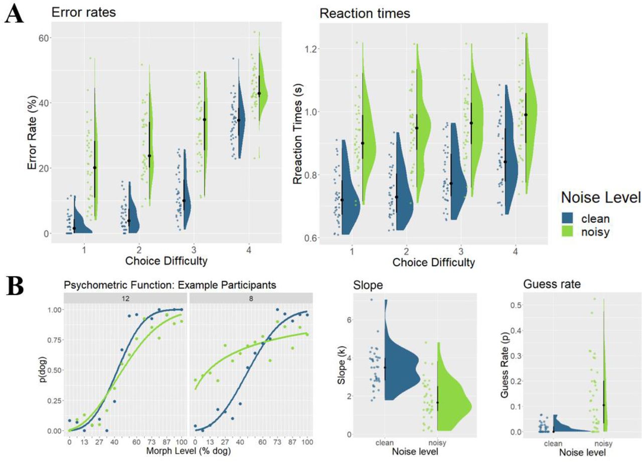
A. Error rates and reaction times. Plots show error rates (left) and reaction times (right) as a function of choice difficulty (1 = easy / far away from decision boundary, 4 = hard / close to decision boundary). Raincloud plots include boxplots centered around the median (black lines), probability density estimates (right half), and raw data (left half), jittered for illustration purposes. B. Psychometric functions. Example choice data from two participants (#12, #8, left). Each dot represents the probability of choosing ‘dog’ (p(dog)), as a function of morph level (expressed in % dog included in the morphed image). Lines represent fitted psychometric functions. The performance of one participant (#8) was heavily affected by noise level, while it was not for the other participant (#12). Estimated slope (k) and guess rate parameters are shown on the right, as a function of noise level (clean, noisy). blue = clean trials, green= noisy trials.
For reaction times, we found that participants responded within 850ms on average (SEM = 13ms, Figure 4A). Similar to error rates, we found very strong evidence for an effect of noise level, choice difficulty, BF10s > 150, with RTs on noisy trials and in high choice difficulty trials being longer. We also found strong evidence for an interaction effect, BF10 = 80.51, again indicating that the effect of noise level decreased with increasing choice difficulty. Only correct trials were used in RT analyses.
3.1.2 Psychometric functions
Next we assessed performance by fitting psychometric functions to the choice data of each participant (Figure 4B). We first tested whether the slope of the function differed between noise levels, and found very strong evidence for steeper slopes on clean trials, BF10 > 150 (mean kclean = 3.48, mean knoisy = 1.81). As expected, this demonstrated that categories are more easily distinguishable on clean, as compared to noisy trials. Next, we tested for a corresponding difference in guess rate, and found very strong evidence for higher guess rates on noisy trials, BF10 > 150 (mean guessclean = 0.01, mean guessnoisy = 0.13). This showed that adding noise leads to substantially more guessing, in addition to a weaker separation of both categories.
In an additional analysis, we then used the estimated threshold (i.e. the point at which choosing cat and dog was equally likely) to determine whether choices were biased towards either category. Morph level ranged from 1 to 16, with the decision boundary being between 8 (most strongly morphed cat) and 9 (most strongly morphed dog). For unbiased choices, thresholds should thus be between 8 and 9 on the morph level scale. To test this hypothesis, we first computed a Bayesian t-test (BayesFactor::ttestBF, Jeffreys prior, r = 0.707) using data from clean images only.
We then extracted the 95% credible interval from the posterior distribution (number of iterations = 100.000), and tested whether this interval includes any values between 8 and 9. If it did, this would indicate that thresholds are indistinguishable from the expected threshold. If it did not, this would indicate that thresholds differ from the expected threshold. For clean trials, the 95% credible interval (95% CI = [8.21, 8.73]) indicated that thresholds were indeed between 8 and 9, as expected. For noisy trials, thresholds were somewhat lower and had a higher variance (95% CI = [7.10, 8.61]), but were still overlapping with the range of expected values. Using different priors (r = 1, r = 1.41) did not change this result. Thus, we concluded that choices were unbiased on clean trials, and that adding noise to the stimuli did not introduce biases.
3.2 fMRI analyses
3.2.1 Zero-order correlations
We first tested whether either of the two theoretical models (clustered coding, equidistant coding) explains the data using zero-order Spearman correlations on clean trials (Figure 5, see Table 1 for an overview of all results). As expected, we found very strong evidence for equidistant coding in ventral visual cortex (r = 0.14, BF10 > 150), and strong evidence for clustered coding in the same region (r = 0.08, BF10 = 80.00). For the MD ROIs, we found evidence for equidistant coding in posterior dlPFC (8C, r = 0.05, BF10 = 4.89), and IPS (IP1, r = 0.06, BF10 = 7.49, IP2, r = 0.09, BF10 > 150). There was anecdotal evidence for a equidistant coding in the anterior dlPFC (p946v, r = 0.04, BF10 = 2.81) and the angular gyrus (PFm, r = 0.05, BF10 = 2.85). No MD ROI showed evidence for clustered coding (all BF10s < 0.58). Thus, we were able to detect stimulus information in visual, parietal, and lateral prefrontal brain regions in clean trials. In noisy trials, we found strong evidence for equidistant coding in the posterior IPS (IP1, r = 0.06, BF10 = 28.14) and moderate evidence for clustered coding in the same region (r = 0.05, BF10 = 8.25). The anterior IPS showed anecdotal evidence for equidistant coding in noisy trials (IP2, r = 0.06, BF10 = 2.85). We also found evidence for equidistant coding in dmPFC (8BM, r = 0.06, BF10 = 5.90). Please note that it remains difficult to attribute results to a specific coding model here, since both candidate models were positively correlated and zero-order correlations do not explicitly control for their covariance. These results demonstrate however that, in principle, we are able to detect both coding formats in both clean and noisy trials.

Raincloud plots (Allen et al., 2021) depict the canonical / zero-order correlation of both models (clustered = blue, equidistant = green) with the data RDM of each ROI. Raincloud plots include boxplots centered around the median (black lines), probability density estimates (right half), and raw data (left half), jittered for illustration purposes. Numbers at the bottom of the plots indicate Bayes factors of a t-test against zero. We only depict results from ROIs that showed evidence for an effect in at least one of the four conditions depicted.
Canonical / zero-order Spearman correlations (r) between the models and the data RDM, including the Bayes factor (BF10) of the corresponding t-test against zero, separately for clean and noisy trials. mPFC = medial prefrontal cortext (SCEF, 8BM), lPFC = lateral prefrontal cortex (8C, IFJp, p9-46v, a9-46v, i68), AI/FO = anterior insula / frontal operculum (AVI), VVC = ventral visual cortex
3.2.2 Hypothesis 1: Visual cortex uses an equidistant coding format
Next, we assessed stimulus coding in ventral visual cortex. We expected the equidistant coding model to explain a unique part of the data variance on clean trials, which we tested using partial correlations (Figure 6). Indeed, we found very strong evidence that the equidistant coding model explained a unique part of the variance on clean trials (r = 0.12, BF10 > 150). Interestingly, for noisy trials, we found moderate evidence against a unique contribution of equidistant coding (r = 0.02, BF10 = 0.33). Directly comparing both results using a paired t-test yielded moderate evidence for a difference (BF10 = 4.97), suggesting that the equidistant coding model better explained data on clean than on noisy trials. These results are largely in line with our predictions. Ventral visual cortex indeed encodes stimuli using an equidistant format on clean trials. We did not detect a unique contribution of equidistant coding on noisy trials however, likely reflecting the fact that stimulus input was strongly degraded.

Raincloud plots (Allen et al., 2021) depict the partial correlations of both models (clustered = blue, equidistant = green) with the data RDM of each ROI, controlling for the other model, respectively. Raincloud plots include boxplots centered around the median (black lines), probability density estimates (right half), and raw data (left half), jittered for illustration purposes. Numbers at the bottom of the plots indicate Bayes factors of a t-test against zero. We only depict results from ROIs that showed evidence for an effect in the manipulation check (Figure 5). For ventral visual cortex and IP2, we also depict brain behavior correlations. The x-axis shows the difference in equidistant coding between noisy and clean trials. The y-axis shows the difference in guessing, as estimated using psychometric functions, between noisy and clean trials. In IP2, the more equidistant coding collapsed in noisy trials, the more participants guessed. This was not the case in ventral visual cortex.
As a control, we repeated the analysis assessing evidence for clustered coding over and above equidistant coding. There was moderate evidence against the clustered coding model explaining a unique part of the data variance on clean trials (r = -0.03, BF10 = 0.09), and the same was true for noisy trials as well (r = 0.01 BF10 = 0.23). The paired t-test yielded moderate evidence for no difference between these values (BF10 = 0.29).
3.2.3 Hypothesis 2: Weak stimulus coding on clean trials in MD regions
For the partial correlation analyses in MD ROIs, we restricted the number of ROIs to those that showed an effect in either clean or noisy trials in the manipulation check reported above, since it can be difficult to interpret partial correlations in the absence of zero-order correlations. This includes parietal cortex (IP1, IP2, and to a lesser degree PFm), dlPFC (8C, and to a lesser degree p946v), and dmPFC (8BM). We expected to see either no evidence for stimulus coding on clean trials, or weak evidence for equidistant coding in these trials. We found evidence for a unique contribution of equidistant coding, after partialling out clustered coding, in parietal cortex (IP1, r= 0.07, BF10 = 3.44, IP2, r = 0.11, BF10 = 37.05, PFm, r = 0.07, BF10 = 12.12, Figure 6), and dlPFC (8C, r = 0.06, BF10 = 3.17, p946v, r = 0.05, BF10 = 2.57), but not in dmPFC (8BM, r =0.00, BF10 = 0.20). As a control analysis, we also tested for evidence for clustered coding after partialling out equidistant coding. For all FPC ROIs, we found evidence against clustered coding (all rs < 0.01, all BF10s < 0.27). The clustered coding model thus failed to explain unique variance on clean trials in all ROIs assessed here. Parietal cortex thus seemed to robustly represent equidistant stimulus information on clean trials, with effects in dlPFC being somewhat weaker. Overall, these findings were largely in line with our predictions, MD stimulus coding on clean trials was either absent, too weak to be detected reliably, or present only in an equidistant format.
3.2.4 Hypothesis 3: Stronger, clustered coding on noisy trials in MD regions
Lastly, we predicted that stimulus coding would be stronger on noisy trials in MD ROIs, and that the information would be represented in a clustered format. Although we expected this effect to be widespread in the MD network, in fact we only found anecdotal evidence for a unique contribution of the clustered format on noisy trials in IFJp (r = 0.05, BF10 = 2.38). For all other ROIs, we found evidence against a unique contribution of clustered coding (all rs < 0.04, all BF10s < 0.63, see Table 2 for full results). Paired t-tests revealed that only IFJp showed evidence for stronger clustered coding on noisy as compared to clean trials (BF10 = 9.50, all other BF10s < 1.05). Thus, of all MD ROIs, only IFJp shows an effect that was in the expected direction, but this finding remains difficulty to interpret since we found no strong evidence for a corresponding zero-order correlation with the clustered model in IFJp (Table 2).
Partial Spearman correlations (r) between the models and the data RDM, including the Bayes factor (BF10) of the corresponding t-test against zero, separately for clean and noisy trials. mPFC = medial prefrontal cortext (SCEF, 8BM), lPFC = lateral prefrontal cortex (8C, IFJp, p9-46v, a9-46v, i68), AI/FO = anterior insula / frontal operculum (AVI), VVC = ventral visual cortex
Unexpectedly, we found evidence for a unique contribution of equidistant coding on noisy trials in parietal cortex (IP2, r = 0.08, BF10 = 4.57), as we had seen in this region on clean trials above (IP2, r = 0.11, BF10 = 37.05). We also found evidence for equidistant coding in dmPFC for noisy trials (8BM, r = 0.06, BF10 = 6.30), which had evidence against equidistant coding on clean trials (8BM, r = 0.00, BF10 = 0.20). Thus the trend was for equidistant coding to go down, from clean to noisy trials, in IP2, and to go up in 8BM. However, paired t-tests revealed moderate evidence against differences across noise levels in IP2 (BF10 = 0.32) and anecdotal evidence against a difference in 8BM (BF10 = 0.80), indicating that these trends were not statistically reliable.
One possible explanation for the relative lack clustered stimulus coding in MD regions on noisy trials might be that the signal-to-noise-ratio on noisy trials was too low to reliably detect stimulus information. We believe this explanation to be unlikely though, as we were able to detect equidistant stimulus coding in parietal and medial prefrontal cortex on noisy trials. It has been shown previously that detecting information in prefrontal cortex is especially difficult (Bhandari et al., 2018), and the fact that we were able to detect stimulus information in prefrontal cortex on noisy trials shows that, in principle, experimental power is high enough to detect such information even in small regions where signals are often weak.
Another possible explanation might be that our analysis approach was biased towards detecting equidistant coding, since the equidistant model has an overall higher variance and complexity than the clustered model and might therefore be easier to detect in correlation analyses. To directly assess this possibility, we performed a number of simulation analyses. Using simulated data, we demonstrate that if anything, our analysis approach was biased towards clustered and against equidistant coding, making our results even more surprising (for full methods and results see Supplementary Analysis 1).
3.2.5 Brain-behavior relations
Overall, the analyses above demonstrated that the unique part of the variance explained by equidistant coding decreases in ventral visual cortex on noisy trials, and that unexpectedly, equidistant coding explains unique variance in anterior IPS (IP2) on both clean and noisy trials. We further found that dmPFC (8BM) showed evidence for equidistant coding on noisy trials. We thus explored these findings further, asking whether (equidistant) stimulus coding in these regions was related to behavioral performance.
For this purpose, we used the parameters of the psychometric function estimated separately for each participant, and computed Bayesian Pearson correlations (BayesFactor::correlationBF, Jeffreys prior, r = 0.33) with the Fisher-z transformed partial correlation between the equidistant coding model and the data RDM. We reasoned that weak stimulus signals would be related to increased guessing. Correlating equidistant coding (after partialling out clustered coding effects) with guess rate on clean trials yielded no evidence for a relation between these variables (ventral visual, r = -0.01, BF10 = 0.37, IP2, r = -0.03, BF10 = 0.42, 8BM, r = -0.23, BF10 = 1.46). Interestingly, on noisy trials we found a relationship between equidistant coding and guessing specifically in IP2 (r = -0.39, BF10 = 9.81), but not in ventral visual cortex (r = 0.13, BF10 = 0.22) or 8BM (r = 0.06, BF10 = 0.28). The direction of this relationship showed that weaker equidistant coding on noisy trials in IP2 was associated with more guessing (Figure 6). To test whether this correlation was specific to noisy trials, we extracted the posterior distribution of the correlation on noisy trials, and tested whether the correlation on clean trials fell within the 95% credible interval of that distribution. The 95% credible interval was CI = [-0.63,-0.09], and thus the correlation on clean trials (r = -0.03) fell outside of this interval. Thus, we have evidence for a difference between both correlations, showing that neural coding of task-related information in IP2 was specifically linked to behavior only on noisy, but not on clean trials.
Demonstrating that correlations differ between noise levels does not directly demonstrate that changes in coding are related to changes in behavior, however. For each participant, we thus computed the degree to which equidistant coding changed across noise levels (r(clean) – r (noisy)), and to which degree guessing changed across noise levels (guess(clean) – guess(noisy)). If a brain region was indeed involved in compensating for increased noise level by enhancing equidistant coding, we would expect that increases in stimulus coding from clean to noisy trials would be associated with less guessing on noisy trials. Indeed, we found evidence for this correlation in IP2 (r = -0.40, BF10 = 10.47, Figure 6) indicating that participants who had stronger equidistant coding of items on noisy compared to clean trials tended not to increase their guessing on noisy trials, whereas participants who failed to increase (or even decreased) their equidistant coding on noisy trials tended to guess more on those trials. There was no such relationship in the other regions showing equidistant coding on noisy trials: ventral visual cortex (r = 0.10, BF10 = 0.24), or 8BM (r = -0.01, BF10 = 0.37).
We then explored whether stimulus coding in IP2 was also related to the slope of the psychometric function, which would indicate a sharper category distinction for participants with stronger stimulus signals. We omitted 8BM here since we found evidence against stimulus coding in clean trials in this region. We found evidence against a relationship between slope and stimulus coding however, r = -.012, BF10s = 0.23. One potential explanation for this finding is that using partial correlations, we remove at least some of the variance related to categorical coding, making it unlikely to find a relation to sharper category distinctions in behavior. Repeating the same analysis using zero-order correlations yielded similar results however, r = -0.04, BF10 = 0.30, making this explanation unlikely.
4. Discussion
4.1 Summary
In this experiment, we investigated whether and how MD regions adapt their coding of task-related information under changing perceptual difficulty conditions. Participants performed a visual categorization task under two different difficulty conditions (clean vs noisy stimuli), and we tested both whether stimuli are represented across the MD network, and in which representational format they are encoded (equidistant or clustered) in each condition. Equidistant coding assumes that information about individual exemplars within a category is preserved, while clustered coding assumes that exemplars within a category are represented similarly, and only information about categories is preserved. We had three hypotheses. First, based on prior research, we expected visual cortex to represent stimuli in an equidistant format in easy trials (Eger et al., 2008; Freedman et al., 2003), and expected a drop in coding strength in perceptually difficult trials (Hypothesis 1). We found evidence for this hypothesis. Second, for MD regions, we expected to see either no or weak equidistant coding of stimulus information on easy trials (Hypothesis 2), reflecting the fact that MD regions are less strongly engaged in easy than in difficult trials (Woolgar, Hampshire, et al., 2011). Although we found little evidence for clustered coding of stimuli in most MD regions, both parietal cortex (IP1, IP2, PFm) and dlPFC (8C, p9-46v) showed evidence for equidistant coding in easy trials. Third, we expected a different pattern of results for perceptually difficult trials, hypothesizing that MD regions would compensate for the increased perceptual difficulty by strengthening stimulus coding and/or clustering these representations (Hypothesis 3). Clustered coding has been shown before in cognitive control related brain regions in non-human primates (Freedman et al., 2003), and based on recent theories (Badre et al., 2021; Botvinick & Cohen, 2014) we reasoned that changing stimulus coding to a more clustered format might be a key neural mechanism of how MD regions compensate for increased task difficulty. However, we found no evidence for this hypothesis. On the contrary, stimulus coding seemed weaker on perceptually difficult trials in most MD regions. Only two regions still encoded stimulus information on noisy trials (dorso-medial PFC, 8BM, anterior IPS, IP2), and did so using an equidistant format. Anterior IPS (aIPS) encoded stimuli equally well in clean and noisy trials, which was remarkable since the ventral visual cortex showed a marked drop in equidistant coding on noisy trials, and may reflect compensation for the weaker input. Additionally, we found that coding in aIPS was related to changes in behavior, with weaker stimulus coding in this region resulting in more guessing.
4.2 Clustered vs equidistant coding in MD
When performing a visual classification task, we need to represent incoming stimulus information, extract relevant stimulus features, and then extract category membership to enable a behavioral response. Prior work on non-human primates demonstrated that this is supported by ventral visual and prefrontal brain regions (Freedman et al., 2003). Ventral visual cortex maintains information about both categories and individual exemplars within these categories, both in humans and non-human primates (Eger et al., 2008; Kriegeskorte, Mur, Ruff, et al., 2008), and our results are largely in line with these findings. The equidistant model, containing information about both categories and individual exemplars, explained response patterns in ventral visual cortex. In contrast, high-level brain regions such as the fronto-parietal cortex are thought to be closer to behavior than to perceptual information. It has been shown that dlPFC and parietal cortex in non-human primates only represent behaviorally relevant stimulus categories, but carry little information about individual exemplars within these categories (Freedman et al., 2003; Freedman & Assad, 2006). For humans, category representations in dlPFC have been shown to be highly abstract, and independent of low-level stimulus features (Mok & Love, 2021), and this reflects the tuning of stimulus representations towards the task goal, i.e. successful classification. Irrelevant differences between exemplars within the same category are discarded and representations are optimized for object classification instead.
This change from more ‘perceptual’ to more ‘behavioral’ representations essentially reflects a dimensionality reduction in stimulus representations, as they move from visual to fronto-parietal brain regions. High-dimensional representations that carry information about the whole perceptual space are transformed into low-dimensional, binary representations that merely carry information about the task-relevant category membership. Recent theories suggest that high-dimensional representations are more easily separable, but are susceptible to noise (Badre et al., 2021; Fusi et al., 2016). Low-dimensional representations have lower separability, but are more robust to noise. For this reason, we hypothesized that low-dimensional clustered stimulus representations would be used in MD regions especially on perceptually difficult trials, where stimulus information is degraded. In perceptually simple trials, we expected to see either no or weaker stimulus coding in comparison.
Our results were only partly in line with these predictions. We observed equidistant stimulus coding on perceptually easy trials in parts of the MD network, namely the parietal cortex and dlPFC, but not the medial PFC and the anterior insula / frontal operculum. Yet, we found no strong evidence for low-dimensional clustered coding in perceptually difficult trials. We found anecdotal evidence for such an effect in the inferior frontal junction (IFJp), but evidence was weak and difficult to interpret since it was based on a partial correlation result in the absence of a corresponding zero-order correlation. Surprisingly, we did find evidence for equidistant coding in the aIPS and dmPFC however.
There are two notable aspects to this finding. First, we were unable to find stronger coding on difficult as compared to easy trials, which has been observed before in MD cortex for stimulus position (Woolgar, Hampshire, et al., 2011), stimulus shape (Woolgar, Williams, et al., 2015) and task rules (Woolgar, Afshar, et al., 2015). On the contrary, information coding in the MD system tended to decrease for noisy trials, except in aIPS in which coding was equally strong coding in both easy and hard trials. Second, we were unable to find evidence for a shift from equidistant to clustered coding as perceptual difficulty increased, which we had predicted on theoretical grounds (Badre et al., 2021), and following work in non-human primates (Freedman et al., 2003; Freedman & Assad, 2006). Instead, aIPS encoded stimuli in an equidistant format on both perceptually easy and hard trials. Given that such a representational format is likely to be more susceptible to noise, finding it on trials in which stimulus information was noisy and degraded was somewhat surprising.
One potential explanation for this might be the difficulty of the classification task overall. Error rates were well over 30% for stimuli close to the decision boundary, and it might be that stimulus and category signals were very weak as a result. Although we expected precisely this fact to drive clustered stimulus representations, we cannot rule out that these representations were too weak to detect in some cases, and our design might have lacked the statistical power to detect clustered coding in perceptually difficult trials. However, our simulations (Supplementary Analysis 1) demonstrated that, if anything, our analysis was more sensitive to finding clustered coding, and less sensitive to finding equidistant coding. Thus, having found evidence for equidistant coding indicates that we could have, in principle, also found evidence for clustered coding as well.
Another, more interesting explanation for this finding is that it might be driven by the type of experimental manipulation we used in this study. By definition, multiple demand regions are more strongly active in difficult, as compared to easy tasks in multiple domains (Assem et al., 2020; Duncan, 2010; Fedorenko et al., 2013). Recently, it has been suggested however that some types of difficulty manipulation might engage the MD regions more than others (Wen et al., 2018). Specifically, this paper suggested that difficulty manipulations that limit or degrade incoming stimulus information (e.g. shorter stimulus presentations, increased noise) might not recruit MD regions as much as manipulations that make stimulus processing harder (e.g. incongruent distractor stimuli, mental rotation, Han & Marois, 2013). This would make sense if MD regions recruit additional attentional resources to compensate for increased processing demands (Duncan et al., 2020), but are not involved in refining stimulus representations themselves. From this perspective, adding noise to degrade incoming information might be a difficulty increase that MD regions cannot compensate for, and are not strongly involved as a result. Obviously, this interpretation is speculative at the moment, and does not immediately account for all the existing literature (Woolgar, Williams, et al., 2015), but could account for the findings reported here. Future research using different, more processing-based difficulty manipulations will be needed to directly compare to these results.
4.3 Difficulty-invariant coding in anterior intraparietal sulcus
Of all the regions assessed in this study, the anterior intraparietal sulcus (aIPS) appeared to have a special role in compensating for increased perceptual difficulty. aIPS is involved in the processing of stimulus features (Grefkes et al., 2002), but also more broadly implied in regulating top-down attention (Humphreys & Lambon Ralph, 2015). Here, it was the only brain region that consistently encoded stimulus information across clean and noisy trials. This is in contrast to stimulus coding in ventral visual cortex, which we only found in clean, but not in noisy trials. Thus, aIPS represented stimulus information in perceptually difficult trials that was undetectable in perceptual brain regions, suggesting a role in maintaining performance under challenging conditions. This pattern of results was only found in aIPS. And although one might expect somewhat weaker or different results in PFC compared to parietal cortex (Bhandari et al., 2018), it would have been reasonable to predict similar patterns of results in the two areas.
Together with the prior research on feature-based attention mentioned above, one interpretation of our results is that aIPS maintains attention to relevant stimulus features under varying difficulties. This would also help explain why aIPS represents stimuli in an equidistant format. Since stimulus features differ between different exemplars within the same category, it would be sub-optimal to discard exemplar-level information and only encode category information instead. Maintaining exemplar-level information instead allows the aIPS to direct attention towards relevant features, in perceptually easy and hard trials.
Additionally, coding in aIPS was predictive of behavior. The more stimulus coding decreased from perceptually easy to difficult trials, the more guessing increased from perceptually easy to difficult trials. Although speculative, this might indicate that successful regulation of feature-based attention, mediated by aIPS, is related to more meaningful, evidence-based decisions. Clearly, more research will be needed to replicate this exploratory finding, yet it suggests that aIPS may be important for successfully classifying visual images that are difficult to perceive.
4.4 Conclusion
Although some results were unexpected, this research demonstrates the value of using model-based RSA to assess adaptive coding in MD regions. While past research focused on whether the strength of representations of visual stimuli (Woolgar, Hampshire, et al., 2011; Woolgar, Williams, et al., 2015) and rules (Etzel et al., 2016; Wisniewski, 2018; Woolgar, Afshar, et al., 2015) change with difficulty, we instead focused on the representational format of stimulus information. Our results suggest that information coding in the MD system does not always increase with perceptual difficulty, but that codes in at least one MD region (the aIPS) may be robust to noisy visual input. Despite our prediction that perceptual difficulty would result in a change in representational format, we instead found that equidistant coding, characteristic of coding in the visual system in easy trials, was in fact maintained in the aIPS on hard trials. Moreover, the maintenance of these veridical codes was predictive of individual behavior. Our data emphasize the value in examining not only whether task-relevant information is encoded under various cognitive conditions of interest, but also in what format.
Author contributions
DW developed the study concept and analysis pipeline, performed the research, analyzed the data, interpreted the data, wrote the article draft, revised the draft, and funded the research. CGG developed the study concept and analysis pipeline, interpreted the data, and revised the draft. SF developed the study concept, interpreted the data, and revised the draft. AW developed the study concept, interpreted the data, and revised the draft. MB developed the study concept, interpreted the data, and revised the draft.
Competing interests
The authors declare no competing interests.
Supplementary Analysis 1: Simulations
Although the two model RDMs both capture stimulus information, they differ significantly in how stimulus categories are encoded. The clustered coding model assumes binary coding of stimulus information, discarding all differences between exemplars and only encoding category differences. The equidistant coding model however assumes that information about different exemplars is preserved in the neural code, and thus contains information about both categories and exemplars.
One effect of these assumptions is that the clustered coding model has an overall lower complexity, with the equidistant model making subtler predictions about representational distances even within the same category. Together with the fact that the equidistant coding model contains exemplar + category information while the clustered coding model contains only category information, this might lead to an unfair competition between these models in the partial correlation analyses used here. The clustered model might be ‘nested’ within the equidistant model, in that it does not contain unique information that is not also contained in the equidistant model. If this were the case, we would expect the clustered model to always be outperformed by the equidistant coding model, which might explain the lack of clustered coding we found.
To test this possibility, we performed a simulation analysis. Specifically, we generated data from either the clustered or equidistant model, and then tested whether our analysis approach was suitable to recover which model generated the data. To do so, we first took the clustered model RDM (range of values = [0,1]), and added varying amounts of random Gaussian noise to each cell of the matrix (mean = 0, sd = [0.01 - 3.00]). This procedure was repeated 1000 times to generate 1000 simulated ‘participants’. These simulated RDMs were then used as input to the same analyses performed on the actual data in the main manuscript, including both the zero-order/canonical and partial correlation analyses. We expected correlations of the simulated RDMs and the clustered model to be higher than with the equidistant coding model, which would indicate successful model ‘recovery’.
Results (Figure S1 A.) indicated that the clustered model better explained the data regardless of noise level in the zero-order correlation analysis, although the equidistant model also explained simulated data to some degree. In the partial correlation analysis, it can be clearly seen that only the clustered model explained the data, while the equidistant model was effectively suppressed and unrelated to the data, irrespective of how noisy the data was assumed to be. We repeated the same analysis, only generating data from the equidistant coding model, and results showed the equidistant model explaining the simulated data better than the clustered model (Figure S1 B). Thus, using our analysis approach, we could recover which model was used to generate the simulated data well, regardless of how noisy data RDMs are assumed to be.
One might argue that these analyses incorrectly assumed that data RDMs are either 100% clustered or 100% equidistant. In reality, data RDMs likely reflect a mix of clustered and equidistant signals, which we did not account for in the above analyses. But what if both models contributed equally to the signal? In this case, both models should explain the data equally well, and this seems a more likely scenario than assuming data are either 100% clustered or 100% equidistant. To test this, we first generated data similarly to the previous two simulations, only now using a ‘mixed’ model in which both the equidistant and clustered models contribute equally. This mixed model was computed by taking the mean of both model matrices, i.e. in each cell of the matrix both models contributed to an equal degree. In addition to being more realistic, this analysis was also more sensitive to detect potential biases towards either model in our analysis approach, as in principle both models should be able to explain an equal part of unique variance in the data in the partial correlation analysis. If one model outperformed the other, our analysis would be biased towards detecting it in our data. Simulation results (Figure S1 C) suggest that the clustered model explains the data slightly better when noise is weak. For noisier data, both models explain the data equally well. Thus, if anything, our analysis approach is slightly biased towards detecting clustered coding (assuming little noise), making our findings of equidistant coding in parietal cortex and other MD regions even more striking.

A. Clustered data. Correlations between simulated data, generated from the clustered coding model, and the two different model RDMs (clustered, equidistant), for different amounts of noise on the data RDMs. B. Equidistant data. The same correlations are depicted, only for data generated from the equidistant model. C. Mixed data. The same correlations are depicted, only for data generated from a mixed model (50% equidistant coding, 50% clustered coding). Zero-order correlations are depicted on the left, partial correlations on the right. Shaded areas represent 90% confidence intervals. The black line represents the noise ceiling, estimated following (Nili et al., 2014), and indicates the maximum correlation that can be expected given a particular level of noise in the data.
Acknowledgments
We would like to thank David Freedman for kindly sharing the stimulus material used in this study. DW was supported by the European Union’s Horizon 2020 research and innovation programme under the Marie Skłodowska-Curie grant agreement no. 665501 and the Flemish Science Foundation (FWO, FWO.KAN.2019.0023.01). CGG was supported by the Spanish Ministry of Science and Innovation (IJC2019-040208-I). SF was supported by the Einstein Foundation Berlin. AW was supported by Medical Research Council (U.K) intramural funding SUAG/052/G101400. MB was supported by an Einstein Strategic Professorship of the Einstein Foundation Berlin, and a GOA of the Special Research Fund of Ghent University (BOF.GOA.2017.0002.03).
References
References


