

Abstract
Functional ultrasound imaging (fUS) is an emerging imaging technique that indirectly measures neural activity via changes in blood volume. To date it has not been used to image chronically during cognitive tasks in freely moving animals. Performing those experiments faces a number of exceptional challenges: performing large durable craniotomies with chronic implants, designing behavioural experiments matching the hemodynamic timescale, stabilizing the ultrasound probe during freely moving behavior, accurately assessing motion artifacts and validating that the animal can perform cognitive tasks at high performance while tethered. In this study, we provide validated solutions for those technical challenges. In addition, we present standardized step-by-step reproducible protocols, procedures and data processing pipelines that open up the opportunity to perform fUS in freely moving rodents performing complex cognitive tasks. Moreover, we present proof-of-concept analysis of brain dynamics during a decision making task. We obtain stable recordings from which we can robustly decode task variables from fUS data over multiple months. Moreover, we find that brain wide imaging through hemodynamic response is nonlinearly related to cognitive variables, such as task difficulty, as compared to sensory responses previously explored.
1 Main Text
1.1 Introduction
A central aim of systems neuroscience is to identify how brain dynamics give rise to behavior. Cognitive behaviors, such as evidence accumulation-based decision making and working memory, involve concerted neural activity distributed across multiple brain areas (Pinto et al., 2019; Steinmetz et al., 2019). While there has been much effort in identifying and assessing the contributions of individual brain areas to specific tasks, fully understanding the neural circuitry underlying these behaviors requires identifying all areas involved and the dynamical interactions between them. Moreover, the brain-wide activity patterns may not follow the well-studied anatomical boundaries (Kaplan and Zimmer, 2020). Therefore, methodologies must be developed that can image large areas of the brain during cognitive behaviors to simultaneously uncover large-scale neuronal interactions and guide further, targeted experimental recordings. Additionally, the computational models we use to interpret large-scale neural activity need to be expanded to identify brain-wide circuits that co-activate, regardless of anatomical constraints.
As the neuroscience community is gearing towards more naturalistic behaviors (Dennis et al., 2021; Krakauer et al., 2017; Egnor and Branson, 2016), there is a need to complement our technical toolkit with methods that can capture brain dynamics unfolding over extended temporal and spatial scales. Before transitioning to naturalistic behaviors, one first needs to standardize appropriate methods that can operate in such challenging experiments by developing these methods in more constrained versions of these general tasks. The well-known two forced alternative choice (2-AFC) decision-making tasks, e.g., evidence accumulation, can serve as a behavioral test paradigm to develop such methods. Freely moving unrestrained rats can be trained to perform it in an operant chamber. Despite its long history, there is still a lot to be discovered in neural mechanisms underlying evidence accumulation (Brunton, Botvinick, and Brody, 2013; Shadlen and Newsome, 2001; Brody and Hanks, 2016).
Understanding the full gamut of brain activity underlying evidence accumulation task requires employing recording technologies that provide access to large swaths of the brain. One such technology is functional ultrasound imaging (fUS). fUS is a recently developed technology that measures changes in cerebral blood volume. The first reports (Urban et al., 2015; Sieu et al., 2015) of using fUS in freely moving rats to image brain activity has established its feasibility, providing for the first time the ability to record hemodynamic changes in cortical and subcortical areas while the rat is moving. Nevertheless, in this freely moving configuration, fUS has been not been used in cognitive tasks, was not used chronically over many months and the studies did not provide an assessment of the magnitude of motion artifacts over extended timescales. In this study, we extend the applicability of fUS in freely moving rats to cognitive behaviors and to chronic imaging up to months. We also show here how such large-scale imaging can discover new areas previously unknown to be involved in evidence accumulation. Importantly, we developed a version of an evidence accumulation task where the trial duration prolongs internal decision processes such that large-scale imaging technologies capture activity across areas, matching the timescale of hemodynamic changes. In our extended version of the evidence accumulation task the animal has to accumulate evidence over 3-5 seconds over a variety of trial difficulties. Training rodents on such complex decision-making behaviors over an extended timescale is challenging but is circumvented by the use of a high throughput behavioral training facility.
Historically, electric potential recordings have been the most accessible method to record the large-scale activity of the brain (Penfield and Jasper, 1954; Dimitriadis, Fransen, and Maris, 2014; Xie et al., 2017). Electrocorticogram (ECoG) has the benefits of portability and high temporal sampling rates. However, even with new advances in high-resolution ECoG (Kaiju et al., 2017; Chiang et al., 2020), it is still constrained in its spatial resolution and penetrating depth. New advances in cortex-wide optical imaging can vastly increase the spatial resolution at the cost of decreased temporal resolution. Optical imaging is similarly constrained in its penetrating depth. Imaging deeper tissue has been achieved by either implantable electrodes or grin lenses to enable deeper optical imaging. However, both solutions are spatially constrained and require an a priori anatomical target, limiting its capacity to discover new brain areas associated with a task.
As an alternative, hemodynamic related imaging has been the dominant modality for wholebrain imaging due to its ability to penetrate deep into the brain. Such technologies, including Functional Magnetic Resonance Imaging (fMRI) and the more recent fUS, provide minimally invasive recordings, as opposed to electrophysiology, which requires physical insertion of probes into the tissue, and optical imaging, which requires that specialized proteins be physically introduced into neurons. This level of un-invasiveness is achieved by indirect measurement of neural activity through changes in the blood flow-related signals in the brain (Ma et al., 2016; Hillman, 2014). The high level of penetration makes hemodynamic imaging ideal for capturing whole-brain networks. The longer physiological time-scale of hemodynamic activity, however, makes hemodynamic imaging less straightforward for analyzing activity during many systems neuroscience behavioral tasks that are designed to probe neuronal-scale activity and thus evolve on the subsecond time-scale. Moreover, technological limitations of common hemodynamic imaging, e.g., the high magnetic field requirement for fMRI has hindered the use of hemodynamic imaging in freely moving animals.
As fUS is based on implants that are, in principle, portable, we turn to fUS to provide deepbrain access in freely-moving rats. fUS (Mace et al., 2013) is a power Doppler-based technique that measures differentials in blood volume over time. fUS signal is highly correlated to neural activity (Nunez-Elizalde et al., 2021). Moreover comparing fUS signals to calcium signals highlights that the ultrasound signal faithfully reflects the neural activity (Aubier et al., 2021; Boido et al., 2019). Additionally, the mechanisms involved in sensing blood flow also trade imaging resolution with the ability to record extremely large areas of the brain, up to 15 mm depth by 16 mm lateral in freely moving rats. Moreover, as opposed to optical recordings, such as wide-field imaging (Grinvald et al., 1986; Scott et al., 2018) fUS can image deep structures simultaneously with the cortex.
fUS stands to play a pivotal role in the future of neuroscience by helping build an integrative platform for probing neural mechanisms underlying cognitive behaviors. To date, it has been used to probe the brain-wide dynamics in a variety of behaviors such as optokinetic reflex (Macé et al., 2018), auditory cortex mapping (Bimbard et al., 2018), hippocampal involvement in movement (Sieu et al., 2015; Bergel et al., 2020), innate behaviors (Sans-Dublanc et al., 2021), saccades guided task (Dizeux et al., 2019), visual cortex mapping (Blaize et al., 2020) and memory-guided behavior (Norman et al., 2021). In all previous studies, the animals were either head fixed or freely moving with the experimenter holding the wires. Ultimately, one would like to have a totally freely moving configuration where the animal can move around unencumbered by the tethering, allowing the animal to behave as naturally as possible and perform learned cognitive tasks.
One necessary advance to fully leverage brain-wide data, such as fUS, is analysis models that can uncover meaningful properties of neural computation during cognitive tasks. This challenge stands in two parts: uncovering independent neural circuits from functional brain data and relating the data and circuit activity to the behavior. The first of these requires new tools that can discover decentralized patterns of activity independent of anatomical boundaries. Recent advances in demixing of neural imaging data leverage graph embeddings of the data to learn independent time-traces that efficiently represent the data (Charles et al., 2021). The second challenge comes from a fundamental difference between sensory and motor areas and brain-wide computation. In sensory and motor tasks that are designed to modulate specific circuits, simple thresholds (i.e., linear decoding) can be used for highly accurate event detection (Norman et al., 2021). Brain-wide cognitive tasks, however, are more complicated and potentially depend on nonlinear interactions between independent circuits. Appropriate analysis toolkits must take into account these non-linearities and the distributed nature of cognitive behaviors.
Using fUS robustly in freely moving rats maintains a number of challenges. The first and foremost of these is in maintaining stable recording over long periods of time and creating a pipeline that can correct motion artifacts, denoise the data, and extract meaningful components of brainwide hemodynamic activity. Moreover, we would like all the aforementioned to hold over a long time period to be able to record chronically as it takes time to train the rats to perform cognitive tasks. Chronic recordings will be critical in gathering a large number of behavioral trials to study brain dynamics opening up the possibility t study learning and to fit behavioral models to the imaging data. We present here a set of solutions that combine both advances in surgical methods to enhance stability in the probe insertion as well as a computational toolkit for fUS pre-processing and basic data analysis. We demonstrate our methodology on multiple recordings spanning two months in the same freely moving rat performing an evidence accumulation task. We demonstrate robust, stable recordings as well as the rich embedding of the task in the hemodynamic signal after our processing pipeline.
1.2 Results
1.2.1 fUS imaging
The imaging technique used in this study is the ultrafast ultrasound imaging developed in (Doppler, 1842; Macé et al., 2011; Montaldo et al., 2010; Urban et al., 2015) and used extensively in many applications (Tiran et al., 2017; Sieu et al., 2015; Demene et al., 2017; Takahashi et al., 2021). This method, based on power doppler (Montaldo et al., 2009; Rubin et al., 1995; Osmanski, Montaldo, and Tanter, 2015), relies on measured returns of a transmitted plane wave to determine the density of blood per voxel. The location of each voxel is computed by the time-to-return at an angle determined via beamforming. As the signal returns are noisy and have low dynamic range for blood moving parallel to the plane wave, multiple returns at different angles of plane wave transmission are used to generate each fUS video frame (Fig 1C).
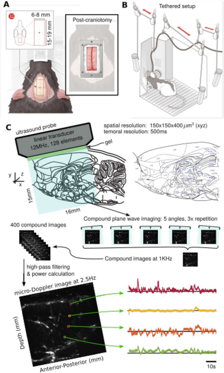
A: Left; Rat skull dorsal surface. The red rectangle represents the area in which the craniotomy is done. Right; Surface view of the headplate positioned on the rat skull dorsal surface after the craniotomy (see Methods and appendix for surgical details). B: Post-craniotomy rat in the operant training chamber tethered with the fUS probe inside the probe holder. The weight of the probe (15 g) is low enough to enable comfortable behavior and movement for the rats. The pulley tethering system allows the animal to move naturally, without any manual intervention. C: The fUS probe we use images a 15 mm×16 mm slice of the brain, including cortical and sub-cortical areas. The probe pulses at 12 MHz, and pulses are distributed across different probe angles to capture angle-agnostic activity, and repetitions to improve signal fidelity. The resulting compound image is produced at 1 KHz, every 400 images of which are filtered and integrated to produce a single μ-Doppler image at 2.5 Hz. The bottom panel depicts an example image (Left) an fUS activity traces over time for four example pixels (Right).
fUS imaging cannot be performed with an intact skull due to the attenuation of the ultrasonic waves by the skull bones. Therefore a craniotomy has to be performed as in Figure 1A. The final configuration of the experimental setup is the post-craniotomy rat freely moving inside a behavioural operant chamber and performing a cognitive task, while being imaged using fUS (Fig 1B). Examples images from the +1 mm medio-lateral saggital plan and examples of time traces showing fluctuations in the cerebral blood volume (CBV) are shown in (Fig 1C).
1.2.2 Behavior on the correct timescale
In order to understand the neural dynamics underlying cognitive behaviors using fUS, it is crucial to choose a cognitive behavior that matches the timescale of the hemodynamic signal measured by fUS. One of the behaviors we are interested in is evidence accumulation based decision making. Conventionally, systems neuroscientists have trained animals to accumulate evidence over relatively short timescales between 100 ms and 1.5 s. Both non-human primates and rodents can be trained to perform this task with high accuracy (Brunton, Botvinick, and Brody, 2013; Shadlen and Newsome, 2001). In its auditory version, the task consists of trials with variable duration during which a stimulus is played on the right and left side of the animal and at the end of the trial, the animal gets rewarded with water if it orients towards the side that have the largest number of auditory clicks. The short time-scale enables the performance of many trials and the ability to characterize the activity of single neurons via, e.g., electrophysiology or calcium imaging Scott et al., 2017; Hanks et al., 2015.
The hemodynamic signal measured by fUS evolve over much longer timescales than either electrophysiology or calcium signals (Nunez-Elizalde et al., 2021). It is thus crucial for fUS, as with fMRI, to be mindful of the design of the behavioral tasks. To match the timescale of fUS, we developed a modified version of the evidence accumulation task wherein the animal is trained to accumulate evidence over a more extended 3-5 seconds (Fig. 2A). Rats are able to perform the task with great accuracy and show behavioral characteristics similar to those observed in shorter timescale trials. The rats are also able to perform the task similarly whether they are tethered or not (Fig. 2C).

A: Example behavior of the previously used Poisson clicks task for rats (Brunton, Botvinick, and Brody, 2013). At each trial an LED lights to indicate the trial start. The rat then uses the center nose poke to initiate the trial, wherein an auditory Poisson click train is played on each of the left and right sides, simultaneously. In the version of the task used here, we extended the duration of the click trains, to play for 3-5 s until the end of click trains and the turning off of the center poke LED. The aforementioned signals to the rat that it should poke the left or right nose poke to indicate a selection, and is rewarded if it selected the side on which the greater total number of clicks were played. B: Frequency response of the total fUS signal averaged over an example area from a fUS imaged behavioral session. Previously used Poisson click trials tend to last approximately 500 ms (Brunton, Botvinick, and Brody, 2013), indicating that the rise/fall time of detectable physiological signatures is constrained to frequencies above 0.5 Hz (where 500 ms is 1/4 wavelength). While this sufficient for electrophysiology and calcium imaging time-scales, hemodynamic signals are much slower. The 3-5 s window in this experiment ensures that much slower physiological responses can be isolated (i.e., the red line of approximately 0.08 Hz). C: Psychometric curve of a tethered rat performing the task is comparable to a untethered rat
When considering the information content of the data, the additional time of the trial significantly lowers the minimum frequency content that can evolve during a single trial. We find that this includes much of the signal frequency content, for example as determined by the average frequency content over a significant portion of the mid-brain (see Fig. 2B for a general quantification and Sup. Fig. 1 for specific brain areas). Extended windows to capture slowly evolving hemodynamics mirrors work in fMRI, e.g., in data-adaptive windowing for correlation computations (Sakoğlu et al., 2010).
Apart from our “ultralong evidence accumulation” behavior, there are other cognitive behaviors that match the timescale of fUS imaging for example parametric working memory, spatial navigation tasks (Fassihi et al., 2014; Aronov and Tank, 2014). With the advent of automated behavioral training, our ability to train rodents on long timescale trials will increase facilitating the use of hemodynamic based imaging techniques and opening up the opportunity to understand neural dynamics over extended spatio-temporal scales.
An important methodological advent in our study is the development and use of a tethering system for the fUS probe that allows the animal to move freely and perform the behavior at the same accuracy and efficiency as without the tethers (Fig. 2C). Previous reports involving fUS in freely moving rodents, involved the experimenter holding the wire by hand. A tethering system with no experimenter interference is crucial for cognitive behaviors that involves self initiated trials. This will also prove crucial when probing brain wide dynamics underlying naturalistic behaviors such as foraging where the behavior of the animal is left to unfold naturally.
1.2.3 Functional ultrasound data curation
Hemodynamic fluctuations operate on the timescale of multiple seconds. The long timescales afford the opportunity for cheap and easy denoising in the form of wavelet denoising (Donoho, 1995). We recommend denoising only along the temporal dimension of the data, rather than image-based denoising of each frame. As wavelet denoising has a computational complexity of T log(T), the total computation is MNT log(T), where MN is the number of pixels in the image, and the MN operations can be parallelized over multiple cores. Image denoising would have a cost of MNT log(N) log(M), which is in general higher than MNT log(T). Moreover, the time-domain signal statistics should more closely match the underlying polynomial assumptions of wavelet denoising (Daubechies, 1992).
Paramount to scientific analysis of data is validating the integrity of the data. As imaging methods advance and are moved to new operating regimes, so too do the potential signal acquisition errors. In addition to typical noise condition, setups enabling freely moving behavior can exacerbate motion-based errors. It is thus necessary to 1) isolate such errors early in the pipeline and 2) devise strategies to either correct such errors or to propagate the uncertainty through to the ensuing scientific analyses. For fUS data, the motion-based artifacts come in two main forms: burst errors (Brunner et al., 2021) and lateral motion offsets.
Burst errors are the easiest to detect. Simple frame-wise norm computations (sum-of-squares of the pixels in each frame) can isolate individual frames that have abnormally large intensities (Fig. 3A). Any outlier detection method can then be applied on these norms, treating any frame with norm greater than a threshold as an outlier. As overall frame intensities do no change dramatically over the course of imaging, a single threshold is sufficient, rather than requiring a local threshold defined by the context of the immediately preceding and ensuing frames. In our case we use a histogram to determine the appropriate decision threshold (Fig 3B, see Methods Section 2.6). In particular we note that the distribution of frames has a fairly sharp fall-off.

A: Burst errors (top, middle frame), or sudden increases in frame-wide image intensity (A, Top, middle), are caused by sudden motion of the animal. Burst errors can be corrected using spline-based interpolation (A, bottom). B: Histograms of frame intensity can be used to easily identify burst frames from using a data-adaptive cutoff (see Methods Section 2.6).
Burst errors can also be corrected, as they tend to occur as single, isolated frames. Simple polynomial interpolation (Brunner et al., 2021) between frames yields smooth video segments (Fig. 3A). Moreover, advanced data analysis methods could simply excise the burst-error frames and robustly compute the necessary statistics/results while treating those time-points as “missing data” (Tlamelo et al., 2021; Pimentel-Alarcón et al., 2016).
Motion correction is more subtle than burst-error correction. We begin with the simplest model for motion in fUS: the rigid-motion model (Heeger and Jepson, 1992; Pnevmatikakis and Giovannucci, 2017). Under the rigid motion assumption, each frame is thought to be offset by a (potentially fractional) number of pixels in each direction. Rigid motion can most easily be assessed via the cross-correlation function of each frame with a reference image. The peak of the cross-correlation determines the shift that induces the maximal correlation with the reference image, and therefore the most likely frame offset. We allow for sub-pixel motion estimation by fitting the offset and scale of a Laplace function to the autocorrelation and using the inferred non-integer offset as the motion estimate (see Methods Section 2.7, Fig. 4A). We note that we did not notice rotational motion, only rigid motion of the probe with respect to the brain.

A: Rigid motion estimation corrects frame-by-frame image offsets via frame-wise autocorrelations (top panel). Frames with high estimated motion correlate with changes in the blood-flow signal, as we quantify with a new metric: the MEPS score. B: MEPS Quantifies the effect of rigid motion error on pixel statistics enabling video stability assessment and evaluating of motion correction. The MEPS computes for each pixel the distribution of intensities for frames tagged as low-motion and frames tagged as high-motion (see methods). Each motion category is then further subdivided into multiple groups, to enable within-versus across-group comparisons. The MEPS score quantifies the ratio of within-group versus across-group differences in these distributions. A score of ‘1’ means that the high-motion frames are indistinguishable from the low-motion frames in aggregate. C: (top) The MEPS value for a session with relatively high motion. The distribution of scores across pixels, both before motion correction (blue) and after motion correction (red). As a comparison, a shuffle test that randomly distributes data to the high- and low-motion tags is shown (yellow). The MEPS score is greatly reduced post rigid motion correction. (bottom) The spatial distribution of the MEPS score pre- and post-motion correction shows how clear anatomical features that create motion artifacts are greatly reduced.
The fUS signal tends to be relatively stable over short timescales and thus only residual motion over long time-scales must be assessed. In performing such analysis, we find that during blocks with large residual motion estimates, the statistics of single pixel time-traces can change significantly (Fig. 4B), indicating that rigid motion does exist, and can be identified via cross-correlations.
Motion correction is often difficult to assess quantitatively. While movies may look more aligned to a human observer, there may be small residual motion that can affect down-stream analysis. To assess motion’s impact on analysis, we assume that during repeated trials in a single session the statistics of single pixels are similar in distribution. In essence, the values at pixel i over time should not have vastly different histograms when conditioned on different sets of frames. We quantify this effect by measuring the change in pixel value histograms for each pixel between high and low motion frames (see Methods Section 2.7). To account for natural variability across the entire session, the high-motion frames and low-motion frames are in turn split into randomly selected subsets. Blocks of frames are selected together to retain the temporal correlation of the signal. The histograms are then compared using an earth-mover’s distance (Haker et al., 2004), with the inter-motion distances (high vs. low) given as a fraction of the average intra-motion distance (low vs. low and high vs. high). For this metric, values closer to one indicate more similar histograms and therefore a lesser effect of motion on data statistics. We denote this metric the Motion Effected Pixel Statistics (MEPS) score.
Our metric enables us to both test the stability of recordings, as well as the effect of postprocessing motion correction. For three of the four recordings spanning two months we found that that the distribution of the metric over all pixels was fairly close to a shuffle-test comparison. This similarity to the shuffle test indicates that the recordings are stable (Sup.Fig 3). Moreover comparing pre- and post-rigid motion correction for these sessions resulted in comparable histograms, indicating recording stability. For the remaining session with very high values, motion correction significantly reduced the metric, indicating much more stable videos post-correction (Fig. 4C).
1.2.4 Decoding of behavioral variables
Using fUS to characterize global brain activity requires a data processing pipeline that can relate the raw data to behavioral variables. Such a pipeline builds on the denoising and motion correction methods mentioned previously. With the registered data, we first provide basic tools to map pixels associated with different aspects of the evidence accumulation decision making task. The first is a comparison between conditions (e.g., activity within and outside of a trial; Fig. 5A-C) and the second is a correlation map that identifies pixels tuned to specific instantaneous events (e.g., reward times Fig. 5D,E).

A: To determine differences between global hemodynamic activity during different epochs, frames during those epochs (e.g., during a trial and between trials) were averaged separately. The difference between the two maps was then taken to produce the difference map comparing two conditions. B: The difference between the average data frame during a trial and between trials demonstrates areas with different hemodynamic activity (computed as in panel A). C: Similarly, the difference between the average data frame within a correct trial versus an incorrect trial demonstrates even more differences, especially in the cortical areas M2 and RSD. D: To determine event-triggered changes in activity, fUS activity was correlated with a synthetic trace representing a derivative of activity time-locked to the event. Here the event was the end of correct trials. A Gaussian shape with a width of 2 seconds (4 frames) was selected. The resulting estimate of the time derivative is shown in the top panel, with red indicating locations with increases in brain activity time-locked to end of correct trials, and green indicating decreases. E: Example event-triggered changes locked to the end (last frame) of correct trials, as computed via event-triggered correlation maps in panel D.

A: The general pipeline for fUS decoding is to first denoise and motion correct the data via the previously mentioned pre-processing steps. Signal extraction then identifies the basic temporal signals from the raw data. Finally decoding, in our case using support vector machines, is applied. B: Signal extraction is accomplished via GraFT (Charles et al., 2021) GraFT is a data-driven decomposition that seeks to describe each pixel’s time-trace in the movie as a sparse linear combination of a dictionary of basic temporal components in the data. GraFT uncovers these basic components via an unsupervised dictionary learning procedure that iteratively updates the time-traces and the spatial profiles (i.e., how much each time-trace is present in each pixel). Key to GraFT is that the pixel decompositions are correlated via a learned graph based on temporal correlations (Charles et al., 2021). C: GraFT uncovers spatial areas exhibiting independent activity. Three example areas (of the 45 learned areas) are shown, and the full complement provide a low-dimensional description of the data.
Comparing between conditions is a simple difference-of-averages (Fig. 5A); The average of all frames in condition two is subtracted from the average of all frames in condition one. The difference removes baseline activity levels constant over both conditions. For example, maps comparing activity within and outside of a trial demonstrate significantly decreased activity in V2 visual cortex (V2MM) (Fig. 5B). Similarly, error trials seem to induce more activity in area Motor Cortex (M2) and Retrosplenial Cortex (RSD) than correct trials (Fig. 5C).
Correlation maps depend on instantaneous events, rather than spans of time. We create correlation maps that average the frames surrounding each event to discover which pixels are most active in the vicinity of those events. To prioritize frames closest to the event, we weigh the frames in the average with an exponential-squared fall-off from the nearest event (Fig. 5D). Furthermore, to differentiate pixels active before and after the event, we weigh frames right before an event with negative values and frames right after with positive values (Fig. 5E). The correlation maps can further be used to compute the responses across brain areas by integrating the computed values over voxels corresponding to registered brain areas (see Methods Section 2.10, Supp.Fig. 6,7,8,9).
While informative, these maps ignore the high degree of temporal correlation between pixels, and do not seek explanatory mechanisms. Thus we expand the data processing pipeline with a signal extraction stage to permit efficient and accurate decoding (Fig. 7A). We leverage recent advances in time-trace extraction from neural imaging data which seeks to identify the independent temporal components underlying the full fUS video (Fig. 7B). This method, Graph-Filtered Timetrace (GraFT) analysis, iterates between updating the time-traces that best represent each pixels time-trace through a linear combination provided by the spatial weights, and then updating the spatial weights based on the new, updated time-traces (Charles et al., 2021). Importantly, GraFT uses a data-driven graph to abstract away spatial relationships within the fUS video to learn large-scale and non-localized activity profiles. The result is a decomposition Y ≈ ZTΦ where the pixelby-time matrix Y is described by the product of a component-by-time matrix Φ that has each row represent one independent time-trace in the data with the pixels-by-component matrix ZT of spatial weights describing which pixels are described by which independent time-traces in Φ.

A: Decoding in- and out-of trial imaging frames can be computed in the learned low-dimensional representation from Figure. 6. We find that classifying frames is much more accurate with a Gaussian Kernel SVM than with a Linear SVM, indicating complex nonlinear activity in fUS brain-wide dynamics. Moreover, the number of consecutive frames used in decoding increases accuracy slightly, indicating non-trivial temporal dynamics. B: Similarly, when decoding hard vs. easy trials (as determined by the difficulty parameter γ), we similarly see a large boost in performance using a nonlinear decoder. In fact the linear SVM performs worse in decoding hard vs. easy trials than it does in determining in vs. out of trial frames, while the nonlinear decoder performs better. C: Same Gaussian kernel SVM decoding as (A) for a second data set two months later shows comparable decoding of in- and out-of trial activity. D: Same Gaussian kernel SVM decoding as (B) for a second data set two months later shows comparable decoding of task difficulty.
The result of GraFT is a reduced description of the fUS video that identifies independently co-active regions (e.g., Fig. 7C, Sup.Fig. 11,12, Supp.Fig. 15). For example we identify RSD being highly co-active within itself and with parts of M2. Importantly, GraFT does not assume spatial cohesion, indicating that the connectedness of the identified co-active areas is truly a product of the data statistics and not an assumption built into the algorithm.
The reduced dimension of the GraFT decomposition enables us to efficiently decode behavioral variables by using the 30-60 time-traces instead of the >20K pixels as regressors. As an initial test we decoded whether a rat was within a trial or out of a trial.
We found that the GraFT decomposition, despite being a linear decomposition of the data, did not yield high decoding levels with a linear support-vector machine (SVM) classifier (Fig. 7A). The same data used in a nonlinear SVM—using a Gaussian radial basis function (RBF) kernel (see methods)—had very high decoding performance (Fig. 7A). We obtained similar results on more intricate cognitive variables, such as decoding whether the trial was difficult or easy, from only the fUS brain images (Fig. 7B) In general, we found that using an RBF SVM on GraFT decompositions of the fUS data was successful in decoding a number of behavioral cognitive variables (Supp. Fig. 16).
1.2.5 Stability over multiple sessions
A major aim of our study is to be able to record from the same rat performing a cognitive task over many months. We therefore asses the stability of our recordings over short and long timescale by comparing fUS data collected in the same rat during sessions spaced days and months apart. We first found that all data could be registered via rigid motion. The estimated movement of the probe between sessions was ≤ ∓0.5 mm in AP, and ≤ ∓1 mm in depth (Fig. 8A). The registration was further validated by comparing the average image (i.e., an ‘anatomical image’) between sessions. The correlation between the anatomical image between sessions was high both between days and across months (Fig. 8B). These shifts allow us to further compare behaviorally dependent measures, such as the changes in event-triggered brain activity, over many months (Fig. 8B, Supp. Fig. 18, 19,6,7,8,9).

A: Rigid motion estimation infers at most only a ±2 mm shift in either depth or the anterior-posterior direction over two months of chronic implantation and recording. Interestingly, AP motion is much more stable, with typical offsets between recording days at < 0.5 mm. B: Image stability can be assessed over multiple months by comparing the anatomical images computed via averaging over time. We note that the anatomy is stable over long time-frames, with very high correlations both between the anatomical images on subsequent days, as well as two months later. C: As the anatomical plane is stable over long time-frames, changes in hemodynamic activity during the decision making task can be detected over the course of chronic recording. The maps of differential brain activation at the start of a trial can be compared between sessions months apart to study
1.3 Discussion
In this paper, we have presented detailed experimental and algorithmic techniques that allow for practical chronic implementation of functional ultrasound (fUS) imaging of the brain in freely moving rodents. The criteria that we have set for the success of our technical protocols is to obtain chronic stable fUS data from rats’ brains, while the animals perform cognitive behaviors in a freely moving manner. Our solution was realized by: 1) devising a surgical protocol that allowed us to open a large craniotomy and stabilize the functional ultrasound probe facilitating brain imaging over an extended time period up to many months, 2) developing and validating a rodent behavior that matches the timescale of the hemodynamic changes measured by fUS, 3) developing motion artifact detection and correction algorithms that further stabilize the fUS images and ensure chronic same plane imaging, and 4) developing appropriate analytical methods to extract brain activity aligned with behavioral events.
To ensure complete clarity and reproducibility of our procedures, we have provided detailed protocols that include step-by-step schematic description of the surgical procedures, open source code for motion detection, correction and data analysis, along with a detailed description of the codes and an up-to-date repository for updated analysis methods. It complements already existing detailed protocols in the literature for fUS imaging in head fixed mice (Brunner et al., 2021).
Although it has been shown before that one can use the functional ultrasound technique in freely moving rodents (Urban et al., 2015; Sieu et al., 2015; Bergel et al., 2018; Bergel et al., 2020; Rabut et al., 2020), prior work was restricted to sensory stimulation or spontaneous movement and not done chronically over many months in the context of cognitive behaviors. Moreover, in previous studies the experimenter was holding the tether while the animal is moving. In our study, we have developed a tethering system that allows animals to move freely without intervention of the experimenter over extended periods of time. This has allowed us to extend the applicability of fUS to complex cognitive behaviors that freely moving rodents are trained to do such as decision making. As there has been an increased interest in freely moving behaviors in conjunction with other naturalistic behaviors such as foraging that includes movement as a crucial component of its execution, optimization and validation of global brain imaging techniques is crucial to obtain stable recording and devising analysis techniques to comprehend brain wide activity.
One primary concern with data from freely moving animals is the potential for severe motion artifacts. Our study took a two-pronged approach to solving this problem. First we introduced new surgical techniques to adhere and stabilize the probe. We further provided motion correction tools that are able to remove burst errors and align frames via rigid motion correction. To assess our motion artifact mitigation, we proposed a metric that quantifies the difference in functional activity during large and small estimated motion translations. This metric is a per-pixel metric, and the distribution of the metric over all pixels provides a measure of how activity is impacted by motion. For three of the four recordings spanning two months we found that the distribution of this metric over pixels was very close to a shuffle test, indicating minimal motion impact even without any motion correction. For the remaining recording, motion correction significantly reduced the metric values, indicating a reduction in potential motion artifacts.
Motion correction is often assessed via correlations of the images to a template frame. Such correlations often rely sharp features in each image for accurate assessment. In fUS, there are fewer internal features to correspond, as opposed to e.g., calcium imaging at a micron scale. Our metric instead relies on temporal statistics to assess correspondences over time. In general we envision this metric complementing spatially-based assessment. We note that we have implemented basic brain-wide rigid motion correction. While significantly reducing the overall motion, as measured by our metric, future work should explore more flexible deformation based correction, e.g., diffeo-morphic mappings (Ceritoglu et al., 2013) used in ex vivo brain alignment, or patch-based affine mappings (Hattori and Komiyama, 2021).
A well known effect of both motion and erroneous motion correction (especially with global, rigid motion) can induce spurious correlations (Fellner et al., 2016; Power et al., 2012) (Sup. Fig. 20). Spurious correlations can make completely unrelated pixels appear correlated: confounding many functional connectivity analyses as used in fMRI (Power et al., 2012). These correlations (derived in Methods Section 2.13 for completeness) depend on the difference-of-means as compared to the sample variance of each pixel. The total number of frames that are affected by motion play a critical factor and demonstrating the importance of stable imaging as we have implemented in our surgery.
Furthermore, the use of component-based analyses have been shown to reduce the effects of spurious correlations (Perlbarg et al., 2007). Our use of GraFT here assists in two ways. First, the graph constructed for GraFT to learn components over are a k-connected graph. Thus weaker correlations become thresholded to zero, removing those edges from the graph. Second, the components learned must have the same time-trace. Thus if the signal with the high/low alternation due to motion or motion over-correction does not match aside from the change in baseline, a component will not be learned.
The benefits of GraFT against spurious motion has a number of limitations. For one, if the difference of means between mixed pixels is large compared to the variance, a step-function like sequence might be learned, however we have noted no such learned component. A second danger is if a large component with very well defined boundaries undergoes motion. In this case, a large number of pixels at the edges on either side of the component would all have a shared time course that is only on (or off) during shifted (or not shifted) frames. This artifact would be picked up by the dictionary learning in GraFT as a unique component with the on/off signature. None of the components we learned displayed this behavior, indicating that for the fUS data analyzed, these effects were well controlled by the mixture of stable recording, pre-processing, and component identification with GraFT.
While the potential for imaging plane offsets (D-V) exists, we do not notice significant deviation as based on longitudinal consistency computed via session-wise average-image correlations Fig. ??C, Supp. Fig. 8B). Additional assessment of D-V stability can be obtained by emerging volumetric fUS recordings (Brunner et al., 2020). These recordings will enable full 3D alignment of the brain between sessions.
Importantly, the tools presented in this work enable chronic recording over multiple months of the same brain areas. While there is the concern of the plane of imaging shifting, both anatomical images (averages over entire videos) and decoding results indicate that the same areas are being imaged two months later. While anatomical and behavioral measures can be consistent, we note that the brain activity itself might change as the animal performs the task. Thus we do expect changes in brain activity, as we note in the event-triggered average and maps estimated over multiple trials. fUS thus can provide a new window with which to study changes in neural processing over long time-scales.
Our analysis tools represent a complete pipeline for fUS that includes all processing steps up to and including decoding analyses. Rather than relying on averaging brain areas from an anatomical atlas, we include in this pipeline a recent unsupervised component detector, GraFT, that identifies groups of independently activated pixels. GraFT, which does not make explicit assumptions on components based on brain areas, was able to find both activity isolated within individual brain areas as well as activity crossing known anatomical boundaries. These components enabled the efficient decoding of behavioral variables. For decoding we opted for a straight-forward supportvector machine decoder. Interestingly, we found that a linear SVM decoder did not achieve sufficient accuracy, while a nonlinear kernel-SVM decoder was able to decode even trial difficulty directly from brain activity. Moreover, using multiple consecutive frames improved decoding performance. This finding raises important question of how brain dynamics encode task variables over time instead of in single snapshots. Further work should thus aim to continue analyzing the relationship between static and temporal brain activity on a global scale during cognitive behaviors.
We expect that just as for other imaging modalities, these tools will expand to include, for example, non-rigid motion correction. We therefore release all our code as an object-oriented library, complete with visualization tools, and the pre-processing and analysis tools used in this work. This toolbox can expand and adapt with the needs of the community, and we hope that as fUS becomes more widespread that other groups will contribute to this code-base.
In the majority of neurophysiological methods, the experimenters have some pre-defined ideas about which brain area to record from and then proceed to implant an electrode or an imaging device or lens to measure from this area. fUS give us the opportunity to record and screen many brain areas simultaneously, thus speeding up the process to find new brain areas involved in behavior. The ability to identify new regions involved in tasks is especially critical in complex behaviors wherein we lack a full understanding of the underlying brain-wide networks involved.
While other modalities, such as positron emission tomography (PET) and Magnetoencephalography (MEG), are being explored for studying brain activity in freely moving subjects, these modalities have other drawbacks. PET relies on radioactive indicators, which creates additional complications and hazards. MEG, like Functional Near-Infrared Spectroscopy (fNIRS), has been applied in humans, however 1) do not scale down to smaller brains and 2) require heavily wired systems that severely restrict motion during imaging.
Large scale electrophysiology, e.g., using neuropixels, has been a transformative technology by enabling the recording of single neurons across multiple brain areas simultaneously. It has recently been combined with fUS in order to derive the transfer function characterizing the hemodynamic signal as a function of the neural signal (Nunez-Elizalde et al., 2021). During behavior, fUS can give us unprecedented insights into global brain dynamics (mesoscale mechanisms) while neuropixels can give us detailed insights into the inner workings of multiple brain areas (microcscopic mechanisms).
The two techniques are thus complementary in providing distinct information about neural mechanisms and brain wide dynamics underlying behavior. Bridging local neural mechanisms and brain wide dynamics is one of the longstanding challenges in systems neuroscience of behavior.
fUS is a mesoscale imaging method that provides access to the whole brain depth in 2D sheets while widefield imaging give us access to the whole dorsal brain surface. These methods are also complementary as they gave us access to different spatial information as well as different signals of activity: one is calcium signal and the other is hemodynamic signal.
One of the crucial aspects of using fUS, as has been noted with fMRI studies, is the time-scale of the behavior. Not every behavior operates on the same time-scale, and appropriate choices in the targets of study must be aligned with the type of brain recordings being used. We have chosen here to extend one such behavior, the evidence accumulation task, to match the timescale of fUS. Luckily, many other important behaviors are, or can be extended to, the multi-second time-scale. Our setup is thus easily applicable to other cognitive behaviors, e.g., parametric working memory and foraging behaviors. The advent of high throughout training techniques and the implementation of large scale lab based naturalistic behaviors will enable future researchers to adopt new tasks and to push the boundary of possible rodent behaviors.
Systems neuroscience is fast approaching the point where local microscopic activity and global brain dynamics must be understood together in complex tasks. fUS offers a vital complementary technique to other imaging modalities that can be implemented in freely moving animals. The combination of global activity imaged with fUS and local recordings targeted to new brain areas discovered via global analyses offers a critical path forward. The capability to scan the brain and identify new regions will only improve as fUS technology improves. Volumetric fUS (Brunner et al., 2020; Rabut et al., 2019), for example will enable near full-brain imaging, and new signal processing for ultrasound (Bar-Zion et al., 2021) have the potential to vastly improve the speed and signal quality of fUS data reconstruction from the ultrasound returns. fUS can also be combined with optogenetics (Sans-Dublanc et al., 2021) so one can study the extent of the perturbations happening as it is increasingly acknowledged that even targeted brain perturbation has global effects (Lee et al., 2010). Given the aforementioned, fUS will complement already existing methods and refine our understanding of how the concerted dynamics of neural activity give rise to behavior.
Conflicts of Interest
The authors declare no conflict of interest.
Author Contributions
AEH and DT: designed and performed the surgeries, designed and built freely moving behavior arena, and performed animal training and data collection. TBM performed the animal behavior analysis. YZ performed the registration of the fUSi data to the rat brain atlas. RS and ASC coded the data processing pipeline, including motion correction, denoising, and demixing. AEH, DT, RS and ASC all performed data analysis. RS and ASC performed all correlation and decoding analyses. ASC and CDB supervised the project. All authors contributed to the writing of the paper.
Data availability
Data used in this study is available at https://osf.io/8ecrf/.
Code availability
The data processing pipeline is coded in MATLAB and available at https://github.com/adamshch/fUSstream.
2 Methods
2.1 Rat Behavioural Training
2.1.1 Training overview
Animal use procedures were approved by the Princeton University Institutional Animal Care and Use Committee and carried out in accordance with National Institute of Health standards. All animal subjects were male Long-Evans rats. Rats were pair-housed and kept on a reverse 12-hour light dark cycle; training occurred in the rats’ dark cycle. Rats were placed on a water restriction schedule to motivate them to work for water reward.
fUS can be performed on behaviors with timescales that matches the timescale of the hemodynamic changes measured which is on the scale of 3 s Nunez-Elizalde et al., 2021. Therefore, it is important to train animals on behaviors matching this long timescale or stretch the temporal dimension by elongating the trials of already established behaviors. There are many behaviors that can be studied for example parametric working memory which already employs long delay periods between two stimuli thus suitable fUS. For this paper, we have extended the evidence accumulation task in (Brunton, Botvinick, and Brody, 2013) to longer trials up to 5 s. In the following, we will delineate the training pipeline that we have established to train rats, in a high throughput manner, on this task that we named “Ultralong evidence accumulation”.
The training proceeds as follows: Approximately 75% of naive rats progress successfully through this automated training pipeline and perform the full task after 4-6 months of daily training. Rats were trained in daily sessions of approximately 90 minutes and perform 100-300 trials per session. We trained rats on extended version of the Poisson Clicks task (Brunton, Botvinick, and Brody, 2013). Rats went through several stages of an automated training protocol. The behavior is done in an operant behavioral chamber with three nose pokes. It is crucial to mention that the final configuration used in this behavior is the right or left port deliver the water rewards and the central nose poke has an LED that turns on and off depending on whether the animal is poking in it or not.
2.1.2 Training Stage 1
In training stage 1, naive rats were first shaped on a classical conditioning paradigm, where they associate water delivery from the left or right nose port with sound played out of the left or right speakers, respectively. After rats reliably poked in the side port, they were switched to a basic instrumental paradigm; a localized sound predicted the location of the reward, and rats had to poke in the appropriate side port within a shortening window of time in order to receive the water. Trials had inter-trial intervals of 1-2 minutes. For the first couple of days, water was delivered only on one side per session (i.e., day 1: all Left; day 2: all Right; etc.). On subsequent days, Left and Right trials were interleaved randomly. This initial stage in the training lasted for a minimum of one week, but with some rats it can be as long as two weeks.
2.1.3 Training Stage 2
In training Stage 2, we aimed at enforcing the center “fixation period” called “grow nose in center”. At first, the rat needed to break the center port Infrared (IR) beam for 200 ms before withdrawing and making a side response. Over time, this minimum required time grew slowly, so that the rat was required to hold its nose in the center port for longer periods of time before allowed to withdraw. The minimum required fixation time grew by 0.1 ms at every successfully complete center poke fixation trial. The clicks were played through the whole fixation period. The offset of the clicks coincided with the offset of the center light, both of which cued the rat that it was allowed to make its side response. Rats are then trained to center fixate for 3-5 s. Premature exit from the center port was indicated with a loud sound, and the rat was required to re-initiate the center fixation. Rats learned center fixation after 3-8 weeks, achieving violation (premature exit from center port) rates of no more than 25% ( violation meant the rat’s nose breaking the fixation for a period longer than 500 ms, the violation time interval was varied among rats with the majority of rats had a violation period around 500 ms and some went down to 100 ms). Unless indicated otherwise, these violation trials were ignored in all subsequent behavioral analyses.
2.1.4 Training Stage 3
In training stage 3, we have Poisson clicks trains played from both right and left ports. Each “click” was a sum of pure tones (at 2, 4, 6, 8, and 16 kHz) convolved with a cosine envelope 3 ms in width. The sum of the expected click rates on left and right (rL and rR, respectively) was set at a constant rL + rR = 40 (for rats) clicks per second. The ratio  was varied to generate Poisson click trains on each trial, where greater |γ| corresponded to easier trials, and smaller |γ| corresponded to harder trials. In this stage we use a γ = 4 which means the easiest trials.
2.1.5 Training Stage 4 to 6
In training stage 4, we add a second type of difficulties meaning we introduce trials more difficult than the trials from stage 3. During the stage, the stimulus being played is a mix of γ = 3 and γ = 4 interleaved trials.
In training stage 5, we add more difficult trials so we have then γ of 1-2-3-4 intermixed.
In training stage 6, we train the rats on the same task that as in stage 5 but beginning to shorten the trial from 5 s to 3 s slowly (with an increment of 100 ms at each trial). The reason to do is that we want the rats to be exposed to trials with variable duration. At the end of this stage the rat is performing the task at variable trials duration (between 3-5 s) and γ (1-2-3-4).
2.1.6 Final Training Stage
In the final stage, each trial began with an LED turning on in the center nose port indicating to the rats to poke there to initiate a trial. Rats were required to keep their nose in the center port (nose fixation) until the light turned off as a “go” signal. During center fixation, auditory cues were played on both sides with a total rate of 40 Hz. The duration of the stimulus period ranged from 3-5 s. After the go signal, rats were rewarded for entering the side port corresponding to the side that have the highest number of clicks. A correct choice was rewarded with 24 μl of water; while an incorrect choice resulted in a punishment noise (spectral noise of 1 kHz for a 0.7 s duration). The rats were put on a controlled water schedule where they receive at least 3% of their weight every day. Rats trained each day in a training session on average 90 minutes in duration. Training sessions were included for analysis if the overall accuracy rate exceeded 70%, the center-fixation violation rate was below 25%, and the rat performed more than 50 trials. In order to prevent the rats from developing biases towards particular side ports an anti-biasing algorithm detected biases and probabilistically generated trials with the correct answer on the non-favored side. The rats that satisfied those final training criteria were the ones that were used for the fUS experiments.
2.1.7 Psychometric
The performance of each rat (pooled across multiple sessions) was fit with a four-parameter logistic function:
 where x is the click difference on each trial (number of right clicks minus number of left clicks), and P(right) is the fraction of trials when the animal chose right. The parameter α is the x value (click difference) at the inflection point of the sigmoid, quantifying the animal’s bias; β quantifies the sensitivity of the animal’s choice to the stimulus; γ0 is the minimum P(right); and γ0+γ1 is the maximum P(right). The lapse rate is (1-γ1)/2. The number of trials completed excludes trials when the animal prematurely broke fixation.
2.2 Surgical Procedures
Animal use procedures were approved by the Princeton University Institutional Animal Care and Use Committee and carried out in accordance with National Institute of Health standards. All animal subjects for surgery were male Long-Evans rats that have successfully gone through the behavioral training pipeline.
2.2.1 Craniotomy and headplate implantation
The surgical procedure is optimized in order to perform a craniotomy that goes up to 8 mm ML x 19 mm AP cranial window on the rat skull and be able to keep it for many months in order to be able to perform chronic recordings. A detailed appendix at the end of the manuscript with the step by step surgical procedure can be found along with illustrations that walk through every surgical step.
In brief, the animal is brought to the surgery room, then placed in the induction chamber with 4% isoflurane. Administer dexamethasone 1 mg/kg IM to reduce brain swelling and buprenorphine 0.01-0.05 mg/kg IP for pain management. Put the animal back to the induction chamber (with 4% isoflurane) until the animal achieves the appropriate depth of anesthesia. The rat hair, covering his head, is shaved using a trimmer. It is important to remove all the hair on the head skin that will be the site of incision afterwards. Put the animal head in the ear bar. Clean copiously the shaved head with alternating betadine and alcohol. From now on, the surgical procedure becomes a sterile procedure. Inject 0.15 ml of a mixture of lidocaine and norepinephrine (2% lidocaine with norepinephrine 20 μg/mL mixture) under the head skin where the incision is planned. The skull overlying the brain region of interest is exposed by making an incision (~10-20 mm, rostral/caudal orientation) along the top of the head, through skin and muscle using a surgical scalpel feather blade. Tissue will be reflected back until the skull is exposed and held in place with tissue clips. The surface skull is thoroughly cleaned and scrubbed using a double ended Volkman bone curette and sterile saline. The cleaning and scrubbing continue until the surface of the skull is totally clean and devoid of signs of bleeding, blood vessels or clotting. Bregma is marked with a sterile pen then a rectangle is drawn using a sterile waterproof ruler. The center of mass of the rectangle is Bregma and it is 19 mm AP x 8 mm ML. Using the surgical scalpel blades, diagonal lines are engraved on the surface of the skull. Metabond (C&B Metabond Quick Adhesive Cement System) is then put all over the surface of the skull (except the area onto which the rectangle is drawn) It is highly advisable to put low toxicity silicone adhesive KWIK-SIL in the region marked by the pen using gas sterilized KWIK-SIL mixing tips to avoid that any metabond covers this area. Using a custom designed positioning device, the sterile headplate is positioned over the drawn rectangle on the surface of the skull. The headplate is pushed down pressing on the skin and Metabond is put copiously t ensure the adhesion of the headplate to the skull surface. The headplate is then slowly unscrewed from the positioning system and the positioning system is then slowly raised leaving the headplate firmly adhered to the skull. The craniotomy can then be performed. Slowly use the piezosurgery drilling (using a micro-saw insert) to remove the skull demarcated by the rectangle drawn by the sterile pen beforehand. The piece of skull cut is then removed very slowly with continuous flushing with sterile saline. The sterile headcover is then screwed to the headplate then a layer of KWIK-SIL is added on the sides of the headplate. The rat is left to wake up in the cage with a heat pad under the cage. Afterwards, the animal takes 10-14 days to recover during which they are observed for any signs of pain or inflammation.
2.2.2 Chronic probe holder insertion
After the recovery period from the surgery, the following steps are performed to insert the mock probe and streamline the fUS imaging so that we do not need to anaesthetize the rat every time we are performing an imaging session. After the recovery from the surgery, the rat is ready for experiments. In order to perform the fUS imaging, there should be a direct access to the open cranial window (that we opened via craniotomy during the surgery). First the rat is anaesthetized. Throughout the whole coming procedure, sterile procedures are to be strictly followed in order to prevent infection of the exposed brain surface. The rat is then put in ear bars centered. The headcover is unscrewed and removed. The brain surface is flushed with sterile saline, then a piece of Polymethelyene Pentene film (PMP), cut to a size that fits the craniotomy, is glued onto the surface of the brain by carefully applying small drops of VETBOND around the sides. It is crucial to make sure that the PMP is tightly glued to the surface of the brain. This step is very crucial to ensure the total minimization of the brain motion during fUS in a freely moving setting. Afterwards the probeholder is screwed onto the headplate. Note that in this case the headcover is not screwed back. Ideally when you look through the probe holder, one can see the brain surface onto which the PMP is glued. We add a mock probe (a 3d printed analogue of the fUS probe) for further protection while the rat is in his cage.
We are able to achieve many months sterility and persistence of the craniotomy due to our multi-layered approach to preserve its integrity: first by employing fully sterile surgical procedures, by sealing it with a sterile transparent polymer and by having a mock probe that gives an extra layer of protection from debris and contaminants. The ability to obtain a reproducible imaging plane across session over many months was obtained due to accurate alignment of the headplate to the skull using our custom designed positioning system, the alignment of the probe holder to the headplate on which it is tightly screwed and the size of the inner surface of the probe holder that prevents vibrations of the fUS probe. In some cases, the inner surface of the probe can be made tighter by putting a clip around it after the fUS probe is inserted inside the probe holder.
2.3 Functional Ultrasound Imaging procedure
When the rat is not doing the task or being trained in its behavioral box, there is a “mock” 3D printed probe that is basically inserted in the probe holder in order for the animal to have the same weight over their head all the time (as explained in the previous section “Chronic probe holder insertion”). The aforementioned configuration gives us the advantage of not having to anesthetize the animal before every behavioral session which preserve the animal welfare and do not alter the animal’s behavioural performance.
Before performing fUS imaging in a trained rat, the rat needs to be acclimated to the new behavioural box in which the imaging will occur and to the weight on its head. In order to do this, incremental weighs are put over the mock probe (every session it is increased 2 grams up to 10 grams) while the animal is training in the new behavioural box where the imaging is going to take place. As soon as the rat reach a performance comparable to its behavioural performance before the surgery, we are ready to perform fUS imaging.
At the time of the experiment, the mock probe is removed. Then sterile de-bubbled ultrasonic gel (Sterile Aquasonic 100 Ultrasound Gel) is put on the actual probe. The real ultrasound probe is then inserted into the probe holder and fixed in place tightly. Before the probe is inserted, the functional ultrasound system is turned on. In order to synchronize the functional ultrasound imaging sequence and the behavior that the animal is performing, we employed a custom designed system composed of an arduino that receives a TTL signal from the ultrasound imaging machine and the behavioural control box and send it to an Open-Ephys recording box. We then use the Open-Ephys software to synchronize those signals. We have validated the synchronization to make sure that both the imaging sequence and the behavioral events are aligned.
We used the same imaging procedure and sequence we used in (Takahashi et al., 2021). The hemodynamic change measured by fUS strongly correlates with the cerebral blood volume (CBV) change of the arterioles and capillaries. It compares more closely to CBV-fMRI signal than BOLDfMRI (Macé et al., 2018). CBV signals show a shorter onset time and time-to-peak than BOLD signals (Macé et al., 2011). fUS signals correlate linearly with neural activity for various physiological regimes (Nunez-Elizalde et al., 2021). We used a custom ultrasound linear probe with a minimal footprint (20 mm by 8 mm) and light enough (15 g) for the animal to carry. The probe comprises 128 elements of 125 μm pitch working at a central frequency of 12 MHz, allowing a wide area coverage up to 20 mm depth and 16 mm width. The probe was connected to an ultrasound scanner (Vantage 128, Verasonics) controlled by an HPC workstation equipped with 4 GPUs (AUTC, fUSI-2, Estonia). The functional ultrasound image formation sequence was adapted from (Urban et al., 2015). The main parameters of the sequence to obtain a single functional ultrasound imaging image were: 200 compound images acquired at 500 Hz, each compound image obtained with 9 plane waves (−6° to 6° at 1.5° steps). With these parameters, the fUS had a temporal resolution of 2 Hz and a spatial resolution (point spread function) of 125 μm width, 130 μm depth, and 200 μm to 800 μm thickness depending on the depth (200 μm at 12 mm depth). We acquired fUS signal from the rat brain at the +1 mm lateral sagittal plane in this study.
2.4 Brain clearing and registration
2.4.1 Perfusion
After the endpoint of each rat, we perfused the animal with ~100-150 ml (or until clear) 1xPBS mixed with 10 U/ml heparin (cold). It was then perfused with ~200 ml 4% PFA in 1xPBS. Then the descending artery was clamped, and the body was tilted by 30° towards the head. The animal was next perfused with 50 ml fluorescence-tagged albumin hydrogel (recipe below). The animal’s head was immediately buried in ice for 30 min. The brain was extracted and further submerged in 4% PFA at 4° C overnight. The brain was then processed using iDISCO clearing protocol (Renier et al., 2014).
Hydrogel recipe: Make 50 ml 2% (w/v) gelatin (G6144 Sigma-Aldrich) in PBS, warm up to 60° C and filter once. Add 5 mg AF647-albumin (A34785 Invitrogen), mix well. Store in 40° C water-bath till use.
2.4.2 Light-sheet microscopy
The brain was cut along the midline into two hemispheres (Sup. Fig. 4). A brain hemisphere was immobilized with super glue in a custom cradle with the medial side facing up. This yielded the best quality towards the midline. The cradle was placed in the chamber filled with DBE of a lightsheet microscope (LaVision Biotech). We used the 488 nm channel for autofluorescence imaging and the 647 nm for vasculature imaging. The sample was scanned with a 1.3x objective, which yielded a 5 um x 5 um pixel size and with a z-step of 5 um. Two light sheets were adopted, and dynamical horizontal focusing was applied. We set a low NA and low dynamical focusing for the autofluorescence channel and a high NA high dynamical focusing for the vasculature channel. Each sample was covered by two tiles with overlap. Preprocessed images combining the dynamical foci were saved.
2.4.3 Registration
We registered fUS images to a standard brain atlas via the alignment of brain vasculature. The registration procedure took two steps: one registered the autofluorescence channel of light-sheet images (taken in the same coordinate reference system as the brain vasculature) to a standard brain atlas (Step 1), and one registered a reference fUS image to a plane of vasculature light-sheet image from the same subject (Step 2). We detail the steps as follows.
Step 1: light-sheet to the rat brain atlas The light-sheet image stacks were first down-sampled to 25 μm isotropic (or a voxel size matching the atlas). The autofluorescence channel of each brain hemisphere was then registered to the corresponding hemisphere of the brain atlas2 (e.g., a high-resolution MRI template) by sequentially applying rigid, affine, and B-spline transformation using Elastix3 (parameter files in folder ‘registrationParameters_LightSheetToAtlas’). The transformations estimated in this step were applied to the vasculature channel. The two hemispheres were then assembled, thereby registering the brain vasculature to the atlas.
Step 2: fUS to light-sheet To localize the fUS position in the brain, we created a 2D vascular atlas by taking the max-intensity projection over 300 μm thickness along the midline of the registered vasculature volume.
We chose a reference session for each subject, calculated the mean intensity at the logarithmic scale, and converted it to an unsigned 8-bit image. The non-brain region above the sagittal sinus was masked out to avoid false signals. This fUS image served as a reference for other sessions to align with and for aligning to the subject-specific vascular atlas.
The fUS image of the same subject was aligned with this vasculature reference using a landmarkbased 2D registration procedure (ImageJ plugin bUnwarpJ4). The matching locations were manually identified by the shape of the big vessels present in both images. To avoid overfitting, we imposed small weights on the divergence and curl of the warping. The generated transformation file can be used to warp any fUS results to the atlas.
2.5 Timing of trials
Assume that a trial runs for time T and that the fUS signal is collected at sampling rate fs. For a particular frequency in the signal to have a fraction 1/L of the wavelength within a trial. Thus the slowest frequency observable by this criterion fmin must satisfy
 where Tfs/2 is the number of effective time-points in the trial given the Nyquist frequency. For L = 4 and fs/2 = 1 Hz, this reduces to fmin = 1/(4T), which, for the trial lengths of T = 0.5, 3, and 5 s correspond to fmin = 0.5, 0.083, and 0.05 s.
2.6 Burst error analysis
Burst errors are defined as sudden, large increases in movie intensity over the entire field-of-view. Such events can be caused, for example, by sudden movements of the animal. Consequently, these events are simple to detect by analyzing the total intensity of the frames, as measured by the ℓ2 norm  for each frame X. We dynamically select a cut-off for determining a burst frame by estimating the inflection point in the histogram of frame-norms loosely based off of Otsu’s method (Otsu, 1979).
2.7 Motion Correction
To ascertain the accuracy of the motion correction algorithm, we estimated the residual motion shift using a sub-pixel motion estimation algorithm based on fitting a Laplace function to the autocorrelation Cij = 〈Xref, X * δ(x – τi,y – τj)〉, where Xref is the z-scored reference image X is the z-scored image with the offset we wish to compute. The Laplace function is parameterized as
 where and {ρ,μx, μy, σx, σy} is the parameter set for the 2D Laplace function, including the scale, x-shift, y-shift, x-spread and y-spread respectively. We optimize over this parameter space more robustly by operating in the log-data domain, i.e.,

 which makes the optimization more numerically stable, gradients are easier to compute and solving for log(ρ) directly removes one of the positivity constraints from the optimization. We further reduce computational time by restricting the correlation range to only shifts of |τi|, |τj| < 25 pixels and by initializing the optimization to the max value of the cross-correlation function {i, j} = argmax(Cij).
This computation relies on a global reference. If few frames are shifted, than the median image of the movie serves as a reasonable estimate. In some cases this is not possible, and instead other references, such as the median image of a batch of frames at start or end of the video. We also provide the option to estimate the motion residual over blocks of frames, sacrificing temporal resolution of the estimate for a less sensitivity to activity. In the case of fUS, the temporal resolution sacrifice is minimal due to the initial round of motion correction from the built-in processing steps.
Optimization for motion correction was performed using constrained interior-point optimization via MATLAB’s built-in fmincon.m function, constraining the Laplace parameters to be positive (λx, λy > 0), and the offset values to be within the pre-defined limits (–μmax ≤ μx, μy ≤ μmax).
Motion correction assessment
Assessing motion correction for functional data can be nontrivial, as the individual pixels themselves may change over time along with the shifts in the full image. To assess motion, we leverage the fact that multiple trials repeat in the data, which implies that the per-pixel statistics should be relatively stationary. This observation means that if we divide the data into low- and high-motion frames, the distribution of pixel values (e.g., as a histogram) should be similar. We measure similarity in this case using the Earth Mover’s Distance (EMD) (Ling and Okada, 2007), a metric historically used to measure the similarity between probability distributions.
Regardless of the assumed stationarity, the data may still have local variability in different epochs. We thus would ideally want to compare the measured distribution deviation relative to a baseline. For this reason we further divide the low-motion frames and high-motion frames into multiple segments and measure an ANOVA-style ratio of the variability between segments in different classes to the variability within each class. Mathematically we divide the values of each pixel at location i,j into groups Glow,k and Ghigh,k’ for k = 1,…,K and k’ = 1,…,K’, i.e., K blocks of low-motion frames and K’ frames of high-motion frames. The groups G aim to include contiguous blocks in order to capture local statistics. We also define the distances dEMD(G1,G2) denotes the EMD between the normalized histograms of groups G1 and G2. The metric we use to determine motion impact on the data is then

A high value for this ratio indicates that the high motion frames follow much different statistics and therefore motion will likely impact the results for any inference using that pixel. As a comparison, we shuffled the data blocks into random groupings and compute the shuffled score for each pixel. The resulting baseline distribution was concentrated in the range [0.5, 2]. Stable data had similar statistics, while data from recordings with larger jumps often resulted in values up to three times greater. We find that motion correction largely reduces these values, however for data with very large jumps the correction does not always result in a perfect baseline when compared to the shuffle test.
This metric provides one useful measurement of motion impact on a pixel-by-pixel bases. Thus it permits assessing local motion effects. Global motion effects can be measured using a second observation: significant motion adds nonlinear variability to the data, which broadens the eigen-spectrum of the data. Specifically we can look at the data’s principal component singular values and compare the curves with and without motion correction.
2.8 Time-trace denoising
To denoise time-traces, we apply standard wavelet-based denoising methods available through MATLAB. Wavelet denoising depends on a number of parameters, including the wavelet class and level at which to denoise (i.e., the time-scale of the finest-resolution details kept). We find that for functional ultrasound data using the ‘sym4’ wavelets at level 6 resulted in adequate denoising.
2.9 Differential map computation
Differential maps compare activated areas under two separate conditions, e.g., in and out of trials or activity during correct or incorrect trials. Assume each frame i can belong to either condition Γ1, Γ2 or neither  The maps were computed in two stages. First the frames Yi corresponding to conditions 1 i ∈ Γ1 and 2 i ∈ Γ2 were separated and averaged separately to obtain an average map for each condition. Second the difference between these two maps were computed. Together the difference map is

2.10 Correlation map computation
Correlation maps measure which image pixels tend to be more or less active during specific events, such as the start of a trial or the delivery of reward. To compute these maps, the weighted average of frames proceeding and succeeding each of the L events at frame τl is computed, using weights  . The average of the weighted average over all events then forms the correlation map.

This computation is equivalent to computing the temporal cross-correlation of a kernel  with a spike train defined by the event times, and then computing the inner product of the resulting vector and each pixel. To differentiate activity directly before and directly after an event from constant activity, we use a kernel that is negative before the event and positive after. In particular we use a Gaussian kernel wk = exp(–k2/4) multiplied by a shifted Heaviside function that is +1 for k ≥ 0 and −1 for k < 0.
We relate the computed correlation to known brain areas by integrating the before (negative) and after (positive) values in the correlation map over the extent of each brain area (Supp. Fig. 6, 7, 8, 9). Mathematically we compute the sums

 where Γk is the set of pixels in the kth brain area (as per the registration procedure), and I(·) represents the indicator function that is 1 if the condition is true and 0 if false. The negative sign in the second computation is simply to reverse the encoding of “before” in Ycorr as negative values. Finally we normalize all the computed values by the maximum per session Smax – max(maxijk(S+), maxijk(S-)).
As different brain areas can have vastly different sizes (i.e., number of voxels covered), for visualization purposes we find it convenient to transform each value in S+ and S- as S(i, j, k) ← S(i, j, k)/(0.01 + S(i, j, k)). The resulting two values provides a summary statistic for each brain area’s correlation to that event. Note that the differential nature of the correlation maps indicates that areas exhibiting activity both before and after the event must exhibit that activity in separate sets of voxels.
2.11 GraFT analysis
To isolate canonical time-traces from fUS data, Graph Filtered Time-trace GraFT (Charles et al., 2021) analysis was applied to the motion-corrected and denoised video matrix Y. Y is a T × P matrix where T is the number of frames in the time-series and P is the number of pixels. The GraFT decomposition factorizes Y into two matrices Y ≈ ΦZ: a T × M matrix Φ consisting of M distinct time-traces and a M × P matrix Z consisting of M spatial profiles indicating how strongly each time-traces is present in a pixel.
Practically, GraFT proceeds in three steps, where the first initializes the learning and the second two are iterated until convergence.
First a graph is constructed where each node represents one pixel and the connectivity (represented by the graph adjacency matrix W) is based on the correlation of the pixel time-traces. Specifically we use diffusion maps (Coifman and Lafon, 2006) for this step.
Second we use a randomly initialized matrix Φ to identify the spatial maps Z using a graph-filtered reweighted ℓ1 (GF-RWL1) procedure (Charles et al., 2021). GF-RWL1 represents a variational inference over Z where a second set of variables γ correlate the values of Z along the graph. Mathematically we iterate over the following two computations until convergence (practically 2-3 computations suffice):
 where α and β are model parameters and [WZ]ij represents the {i.j}th element of the graph values prjected once through the graph adjacency matrix W.
Third the time-traces are updated given the new spatial maps as
where η1, η2, and η3 are optimization trade-off parameters and is the previous estimate of Φ. This optimization is composed of four terms: the first enforcing data fidelity, i.e., that the decomposition should match the data, the second penalizing unused time-traces to automatically prune extra components, the third to constrain the time-traces away from being too correlated, and finally the fourth induces a slowness to the learning over iterations that stabilizes the full time-trace learning procedure.


The initial number of components is pre-set as M. For fUS data we set M = 30, 45, 60 and found minor improvements on decoding and no significant change in variance explained.
2.12 Decoding of behavioral variables
Decoding of behavioral events is performed after pre-processing and the video decomposition using GraFT. As an example we describe here the procedure for decoding in- and out-of trial frames, however the same procedure was used for all decoding, replacing frames in both categories with appropriately partitioned data. To create target labels zi, we label the in-trial frames as zi =1 and out-trial frames as zi = −1. Since the variation of the signal always reflects more information than a static snapshot, we use a moving window of the last N – 1 frames to decode the frame class (e.g., in/out of trial). Additionally, in order to reduce the impact of noise and computational complexity, the decoding is performed on the reduced dimensionality provided by the GraFT timetraces (see previous methods section). We demonstrate this process with linear decoding as an example. Defining the target as a linear combination of the last N frames Yi, i = 1,…, N we have
 where we use the fact that each data image Yi can be defined as a linear combination of the spatial maps Z with weights
  , as per the GraFT decomposition. The dimensionality of the initial decoder d can be reduced from NP to NM. More generally, the data vectors [Φi, Φi-1,…, Φi-N+1]T can be classified as per their labels zi using other methods. In particular we applied both a Linear SVM and a Gaussian Kernel SVM in the decoding.
Two main parameters influence the decoding procedure are the number of past frames used in the decoding N, and the number of GraFT components M. We compared the decoding results of different N and M. N we swept from N =1 (i.e., using only the current frame) to N = 20. In some cases, for example in decoding correct and incorrect trials, N > 10 exceeded the trial length, so a maximum of N = 5 was used. When decoding the trial difficulty, since the interval between two trials is always 7 frames in our data, a maximum of N = 7 was used to guarantee a good generalization ability of the decoder.
The second parameter M that influences decoder performance actually a parameter of the decomposition. The number of GraFT components M modifies the decoding performance based on the overall information and potential complexity of the reduced space. In our experiments, M was set to M ∈ {30, 45, 60}. We find that when N is small, larger M leads to a little higher precision, however this difference decrease as N becomes larger.
In general, we find that the non-linear SVM always performs better than the linear SVM. When applying a Gaussian Kernel SVM, there are two hyperparameters connected with its performance. One is the scale of the Gaussian kernel, and another is the box constraint, which controls the maximum penalty imposed on margin-violating observations. Using the function fitcsvm in MATLAB, and setting the input argument ‘OptimizeHyperparameters’ as ‘auto’, we automatically find the optimal hyperparameters via five-fold cross-validation.
2.13 Spurious correlations due to motion
One factor to consider when quantifying the effect of motion is the possibility of spurious correlations across an image, as seen in fMRI (Power et al., 2012). To illustrate the problem, consider four pixels p1(t),p2(t),p3(t),p4(t), where p1(t) and p1(t) are neighboring and p3(t) and p4(t) are neighboring. Furthermore, assume for the moment that all pixel time-traces are independent, but with different mean values, i.e.,  . As all pixels are independent, ρ(pi, pj) = 0 for all pairs of pixels. We specify Γ ⊂ [1,…, T] as a set K < T times wherein shifts due to motion (or unstable motion correction) effectively mix neighboring pixels. In this case we can now specify
 and similarly

Note that the set Γ specifies the same times for both z12(t) and z34(t) as the motion is global. We can now compute the correlation between the motion-influenced pixels z12(t) and z34(t).

First note that the sample average
 and similarly for z34(t). The sample co variance is then

We can immediately see that in a trivial case of μ2 = μ4 = 0 and μ1 = μ3 = b, we have a non-zero covariance  . Similarly for μ1 = μ4 = 0 and μ2 = μ3 = b, we have a non-zero covariance
  . Depending on the sample size T, these values may be small—depending on the exact value of the non-zero pixel’s amplitude b—but significant.
To compute the full correlation, we also need the denominator of ρz, which depends on the sample vairances of z12(t) and z34(t).
 and similarly for z34(t). Note that the variance is essentially the weighted average of the variances of p1(t) and p2(t), with an additional factor depending on the difference-of-means.
The full correlation can now be written, however for previty we assume the following: μ1 = μ3, μ2 = μ4, and σ1 = σ3 = σ2 = σ4 = σ.

This expression emphasizes a critical point: as the variances of the independent signals shrink with respect to the difference of means, motion can induce a correlation that grows with respect to the fraction of motion-affected frames.
2.14 fUS code-base
Reproducible results are a cornerstone of scientific progress. Moreover, practical and available resources are critical to enhancing the capabilities of labs seeking to implement and use new technologies. We thus created an object-oriented code-base in MATLAB that contains all the methods discussed here and serves as a foundation for future advances for fUS methods. The code is written to be easily used, expandable, and capable of analyzing both single and multiple recordings, i.e., from chronic implantation as described in this work.
3 Supplementary Figures

Additional examples of fUS frequency content as compared to the observable signal given long (3-5 s) and short (500 ms) trials. Signals are shown for a variety of brain areas, as registered to a standard atlas.

Schematic figure of motion estimation using Laplacian fits to the crosscorrelation function. Low spatial resolution (left) or high noise levels (right) can create uncertainty in sub-pixel motion estimation when looking for the maximum value in a spatial autocorrelation function (displayed as bar plots in each plot to capture the pixelated nature of the computed function). We fit a Laplace function (red dashed lines) to the autocorrelation function to capture the ideal peaky behavior of image correlations. The estimated offset of this function then becomes the sub-pixel motion estimate
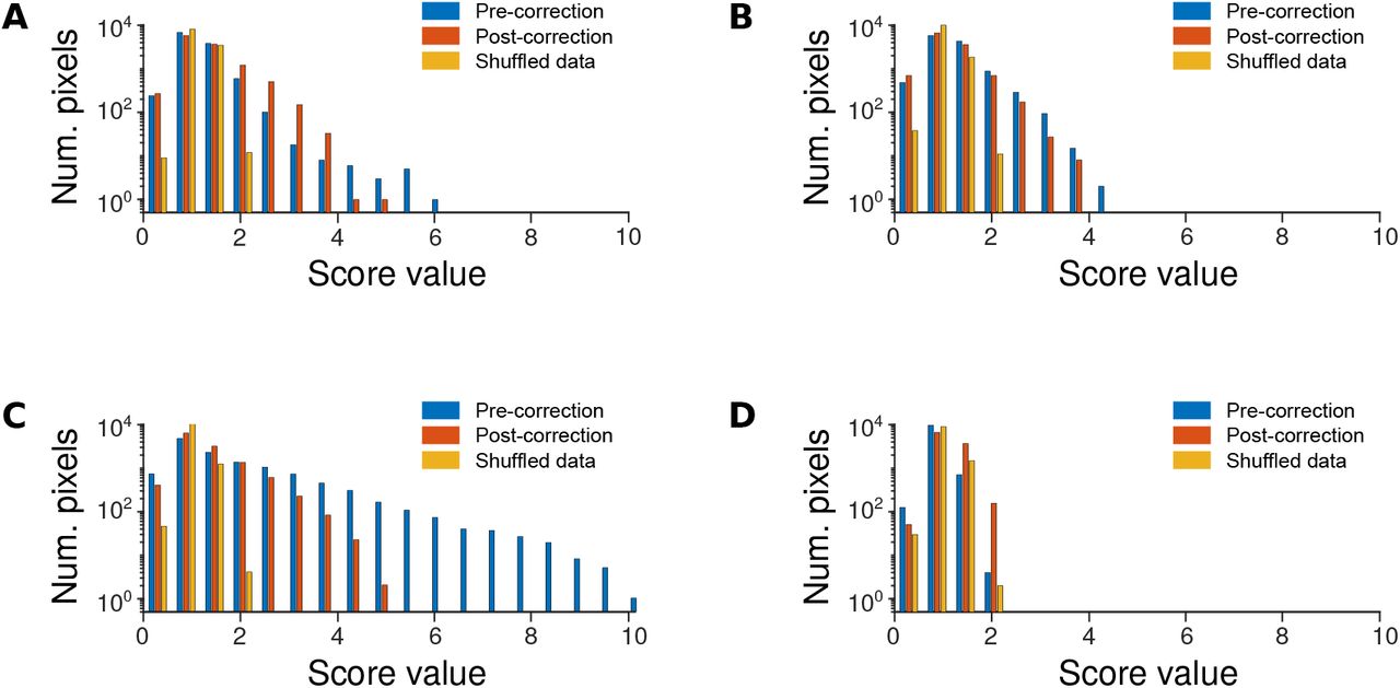
Motion metrics for four different fUS recording session spanning two months. Each plot displays the metric values as a histogram over pixels for the raw data (blue), the motion corrected data (red) and the shuffle test (yellow). Well corrected data tended to stay below values of 3, while data with larger jumps could reach values at twice that level. The shuffled data tended to stay below a value of 2, indicating that there are additional correlations in the data that might affect this metric, however overall it enables an “at-a-glance” assessment of motion contamination: if the uncorrected distribution is much broader than the post-corrected distribution, motion correction is likely required.

fUS images registration: first step is rat brain perfusion followed by iDISCO clearing then light sheet imaging of the cleared brain vasculature. The fUS image is registered to the vasculature image then both fUS and vasculature images are registered to a common standardized rat brain atlas
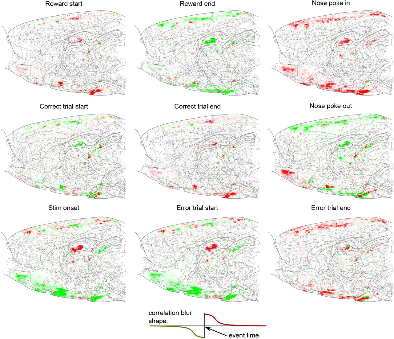
Differential correlation images computed for different trial events. Each image displays the correlation image computed by averaging frames with respect to the correlation shape below, where green indicates more activity right before the event, and red indicates more activity right after the event.

Integrated activity in the correlation maps such as shown in Supplementary Figures 5, 18, 19. Activity before and after is integrated over the physical area corresponding to registered atlas components. Areas with activity both before and after indicate separate areas within the same brain area that are active before or after the event, as constant activity is removed by the correlation computation. Activity is shown on a normalized scale, shrunk by x/(0.01 + x) to normalize for the differences in brain area sizes.

Same as Supplementary Figure 6 for the second session.

Same as Supplementary Figure 6 for the third session.

Same as Supplementary Figure 6 for the fourth session.
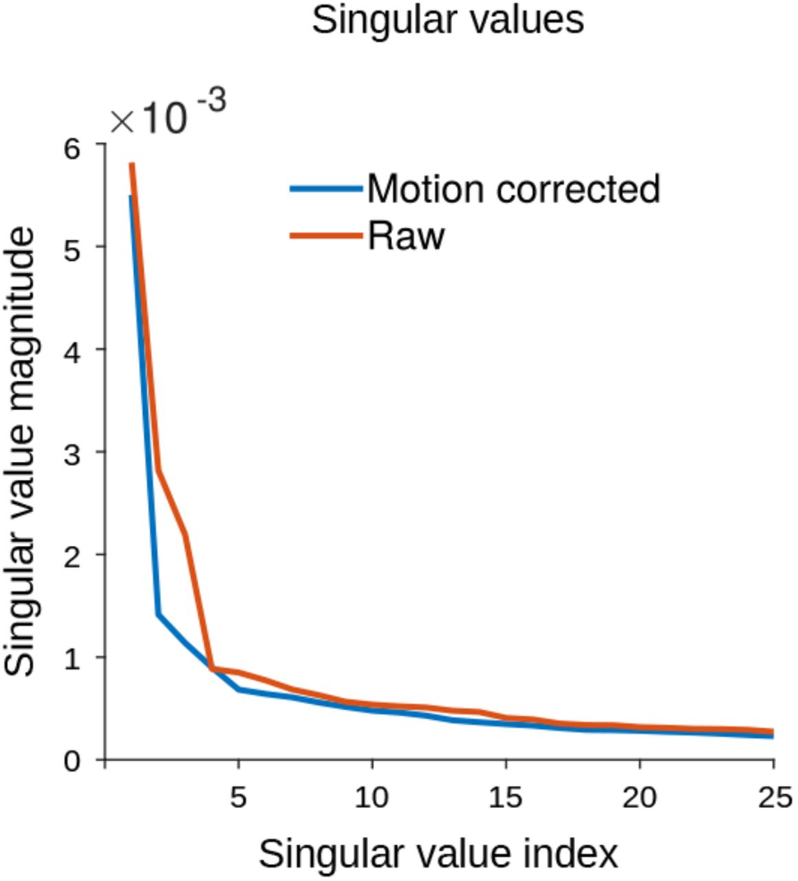
The singular value spectrum of the data is reduced post-motion correction. This is an expected result, as translational motion is known to artificially inflate video dimensionality.
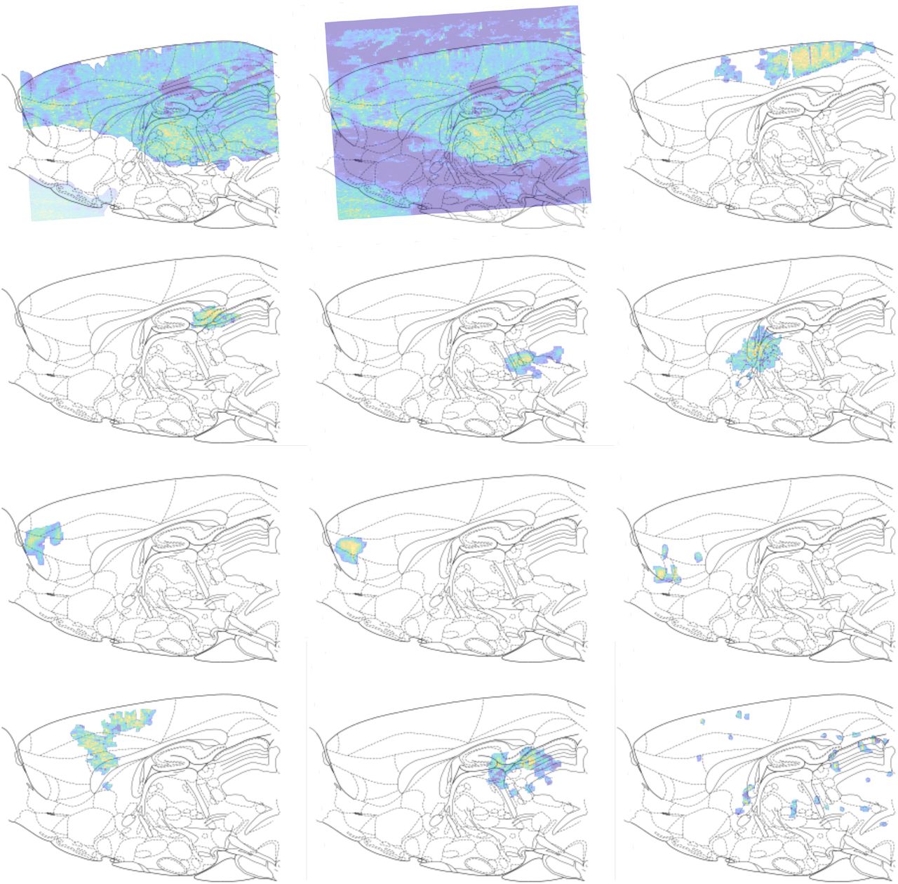
Spatial profiles (independently active areas) extracted using completely unsupervised learning on the motion-corrected and denoised fUS data. We note that the first two profiles capture image-wide background levels of activity, while the remaining profiles begin to capture more localized activity pattern. GraFT, in particular, extracts both activity that seems to be well localized within single brain areas, as well as many activity patterns that appear to recruit across brain areas.

(continued from Supp. Fig. 11). Spatial profiles (independently active areas) extracted using completely unsupervised learning on the motion-corrected and denoised fUS data.
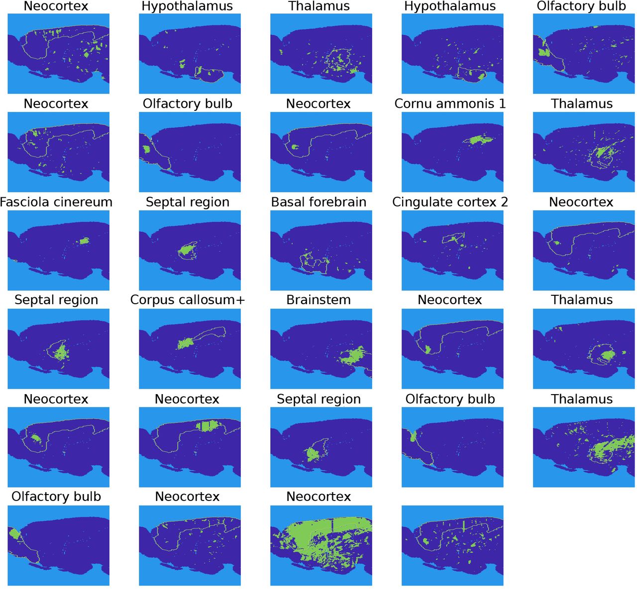
Comparisons of spatial profile overlaps (independently active areas) extracted using completely unsupervised learning compared to the brain region with the highest pixel overlap. Titles designate the name of the most overlapping region, outlined in the figure.

Quantification of overlaps between spatial profiles identified via unsupervised learning and anatomically registered brain regions. Color designates percent of pixel overlap between spatial profiles (components in GraFT) and each brain region.

Time traces identified in fUS data using GraFT.
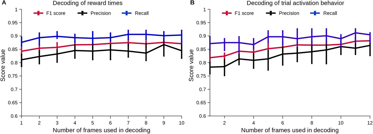
Decoding of additional behavioral variables from decomposed fUS data.

Decoding of in/out of trial frames using different numbers of components in the GraFT decomposition. Frame rate is 2 Hz.
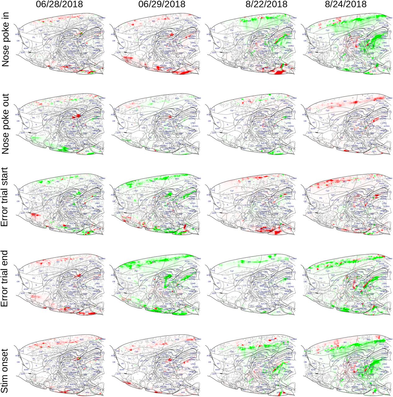
Correlation maps for various behavioral events over four sessions spanning two months. Correlations are computed as in Supplementary Figure 5. Rats were fully trained and had, overall, stable behavior by the time of the first session shown here.

Correlation maps for various behavioral events over four sessions spanning two months (continued from Supp. Fig. 18).

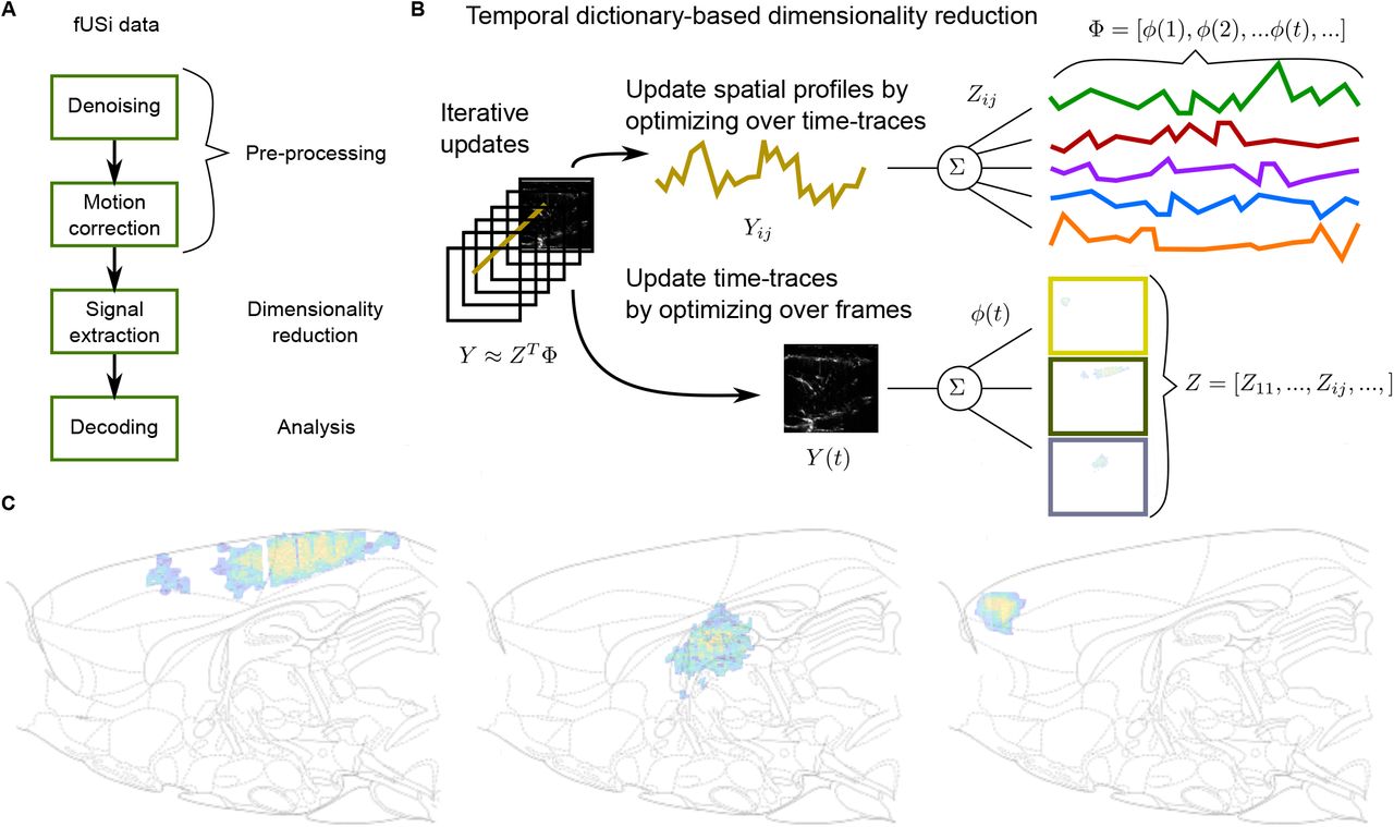
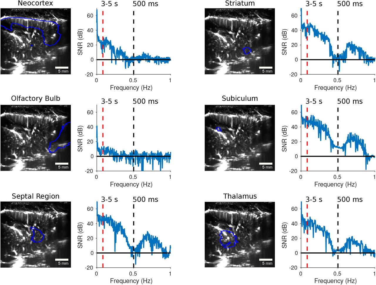
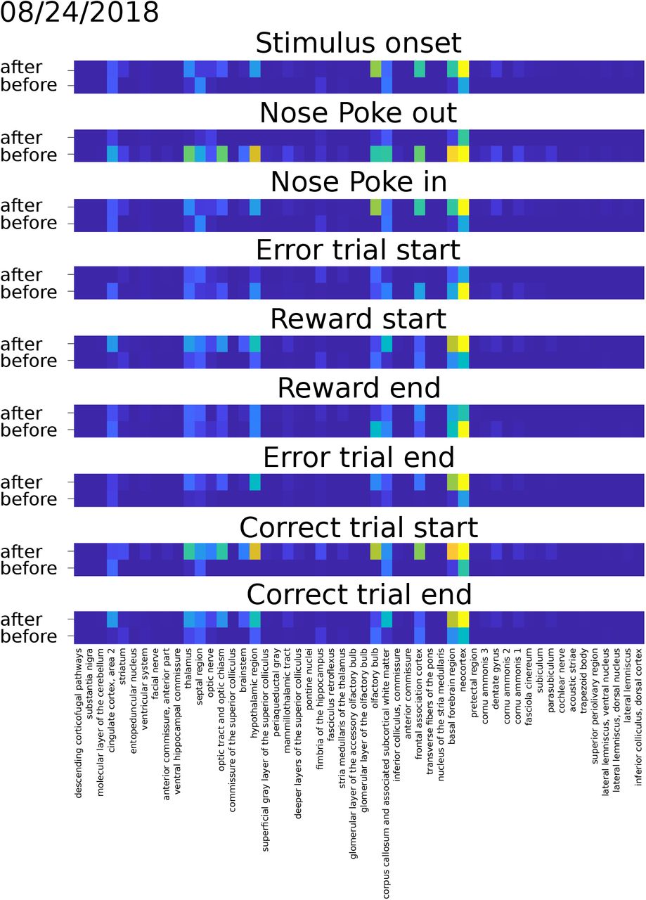
Spurious correlations. A: when two vectors z12 and z34 contains elements from different vectors, interleaved due to motion (or over-correction of motion), differences in amplitudes can create spurious correlation. B: Spurious correlations can be positive (left) due to colinear alignment, they can be negative (middle) due to anti-linear alignment, and they can even influence otherwise correlated vectors (right).
Acknowledgements
The authors would like to thank Alan Urban, Gabriel Montaldo, Emilie Macé for advice concerning functional ultrasound imaging, Diogo Guerra for the surgical procedures illustrations, Emily Jane Dennis for help with the registration and the rat brain atlas, Princeton University Physics Department Workshop, Charles Kopec, David Tank, Brody lab animal training technicians. AEH acknowledges support by NIH grant 1R21MH121889-01.
References
- [1].↵
- [2].↵
- [3].↵
- [4].↵
- [5].↵
- [6].↵
- [7].↵
- [8].↵
- [9].↵
- [10].↵
- [11].↵
- [12].↵
- [13].↵
- [14].↵
- [15].↵
- [16].↵
- [17].↵
- [18].↵
- [19].↵
- [20].↵
- [21].↵
- [22].↵
- [23].↵
- [24].↵
- [25].↵
- [26].↵
- [27].↵
- [28].↵
- [29].↵
- [30].↵
- [31].↵
- [32].↵
- [33].↵
- [34].↵
- [35].↵
- [36].↵
- [37].↵
- [38].↵
- [39].↵
- [40].↵
- [41].↵
- [42].↵
- [43].↵
- [44].↵
- [45].↵
- [46].↵
- [47].↵
- [48].↵
- [49].↵
- [50].↵
- [51].↵
- [52].↵
- [53].↵
- [54].↵
- [55].↵
- [56].↵
- [57].↵
- [58].↵
- [59].↵
- [60].↵
- [61].↵
- [62].↵
- [63].↵
- [64].↵
- [65].↵
- [66].↵
- [67].↵
- [68].↵
- [69].↵


