Estimation of the firing behaviour of a complete motoneuron pool by combining EMG signal decomposition and realistic motoneuron modelling

Abstract

Our understanding of the firing behaviour of motoneuron (MN) pools during human voluntary muscle contractions is currently limited to electrophysiological findings from animal experiments extrapolated to humans, mathematical models of MN pools not validated for human data, and experimental results obtained from EMG decomposition. These approaches are limited in accuracy or provide information on only small partitions of the MN population. Here, we propose a method based on the combination of high-density EMG (HDEMG) data and realistic modelling for predicting the behaviour of entire pools of motoneurons in humans. The method builds on a physiologically realistic model of a MN pool which predicts, from the experimental spike trains of a smaller number of individual MNs identified from decomposed HDEMG signals, the unknown recruitment and firing activity of the remaining unidentified MNs in the complete MN pool. The MN pool model is described as a cohort of leaky fire- and-integrate (LIF) models of MNs scaled by a physiologically realistic distribution of MN electrophysiological properties and driven by a spinal synaptic input, both derived from decomposed HDEMG data. The MN spike trains and effective neural drive to muscle, predicted with this method, have been successfully validated experimentally. Representative applications of the method are also presented for the prediction of activity-dependant changes in MN intrinsic properties and in MN-driven neuromuscular modelling. The proposed approach provides a validated tool for neuroscientists, experimentalists, and modelers to infer the firing activity of MNs that cannot be observed experimentally, investigate the neurophysiology of human MN pools, support future experimental investigations, and advance neuromuscular modelling for investigating the neural strategies controlling human voluntary contractions.

Author Summary Our experimental understanding of the firing behaviour of motoneuron (MN) pools during human voluntary muscle contractions is currently limited to the observation of small samples of active MNs obtained from EMG decomposition. EMG decomposition therefore provides an important but incomplete description of the role of individual MNs in the firing activity of the complete MN pool, which limits our understanding of the neural strategies of the whole MN pool and of how the firing activity of each MN contributes to the neural drive to muscle. Here, we combine decomposed high-density EMG (HDEMG) data and a physiologically realistic model of MN population to predict the unknown recruitment and firing activity of the remaining unidentified MNs in the complete MN pool. In brief, an experimental estimation of the synaptic current is input to a cohort of MN models, which are calibrated using the available decomposed HDEMG data, and predict the MN spike trains fired by the entire MN population. This novel approach is experimentally validated and applied to muscle force prediction from neuromuscular modelling, and to investigate neurophysiological properties of the human MN population during voluntary contractions.

INTRODUCTION

During voluntary muscle contractions, pools of spinal alpha-motoneurons (MNs) convert the synaptic input they receive into a neural command that drives the contractile activity of the innervated muscle fibres, determining limb motion. Identifying the recruitment and firing dynamics of MNs is fundamental for understanding the neural strategies controlling human voluntary motion, with applications in sport sciences (Felici & Del Vecchio, 2020; Watanabe, K. et al., 2021; Maeda et al., 2021), and neurological and musculoskeletal rehabilitation (Jordanić et al., 2016; Fang et al., 2020; Pilkar et al., 2020; Kisiel-Sajewicz et al., 2020; Nishikawa et al., 2021). Determining the MN-specific contributions to the MN population activity also allows more realistic control of neuromuscular models (Callahan et al., 2013; Potvin & Fuglevand, 2017; Kim & Kim, 2018; Carriou et al., 2019), investigation of muscle neuromechanics (Waasdorp et al., 2021; Martinez-Valdes et al., 2021), prediction of limb motion from MN-specific behaviour (Chen et al., 2020), or improvement in human-machine interfacing and neuroprosthetics (Farina et al., 2017; Farina et al., 2021).

Our understanding of MN pool firing behaviour during human voluntary tasks is however currently limited. While the MN membrane afterhyperpolarization and axonal conduction velocity can be inferred from indirect specialized techniques (Freund et al., 1975; Dengler et al., 1988), most of the other electro-chemical MN membrane properties and mechanisms that define the MN recruitment and discharge behaviour cannot be directly observed in humans in vivo. Analysis of commonly adopted bipolar surface EMG recordings, which often lump the motor unit (MU) trains of action potentials into a single signal assimilated as the neural drive to muscle, cannot advance our understanding of the MN pool activity at the level of single MNs. Our experimental knowledge on the remaining MN membrane properties in mammals is therefore obtained from in vitro and in situ experiments on animals (Heckman & Enoka, 2012). The scalability of these mechanisms to humans is debated (Manuel et al., 2019) due to a systematic inter-species variance in the MN electrophysiological properties in mammals (Highlander et al., 2020). Decomposition of high-density EMG (HDEMG) or intramuscular EMG (iEMG) signals (Holobar & Farina, 2014; Negro, Muceli et al., 2016) allows the in vivo decoding in human muscles of the firing activity of individual active motoneurons during voluntary contractions and provide a direct window on the internal dynamics of MN pools. Specifically, the non-invasive EMG approach to MN decoding has recently advanced our physiological understanding of the neurophysiology of human MU pools and of the interplay between the central nervous system and the muscle contractile machinery (Del Vecchio et al., 2019; Oliveira & Negro, 2021)

Yet, the activity of all the MNs constituting the complete innervating MN population of a muscle cannot be identified with this technique. High-yield decomposition typically detects at most 30-40 MNs (Del Vecchio et al., 2020), while MU pools typically contain hundreds of MUs in muscles of the hindlimb (Heckman & Enoka, 2012). The small sample of recorded MNs is besides not representative of the continuous distribution of the MN electrophysiological properties in the complete MN pool with a bias towards the identification of mainly high-threshold MUs. The samples of spike trains obtained from signal decomposition therefore provide a limited description of the role of individual MNs in the firing activity of the complete MN pool.

To allow the investigation and description of specific neurophysiological mechanisms of the complete MN population, some studies have developed mathematical frameworks and computational models of pools of individual MNs. These MN pool models have provided relevant insights for interpreting experimental data (Fuglevand et al., 1993; Dideriksen et al., 2010), investigating the MN pool properties and neuromechanics (Cisi & Kohn, 2008; Negro & Farina, 2011; Farina et al., 2014), neuromuscular mechanisms (Watanabe, R. N. et al., 2013; Potvin & Fuglevand, 2017), and the interplay between muscle machinery and spinal inputs (Dideriksen et al., 2011). However, none of these MN pool models have been tested with experimental input data, instead either receiving artificial gaussian noise (Negro & Farina, 2011), sinusoidal (Farina et al., 2014) or ramp (Fuglevand et al., 1993) inputs, inputs from interneurons (Cisi & Kohn, 2008) or feedback systems (Dideriksen et al., 2010). These MN pool models have therefore never been tested in real conditions of voluntary muscle contraction. The forward predictions of MN spike trains or neural drive to muscle obtained in these studies were consequently not or indirectly validated against experimental recordings.

The MN-specific recruitment and firing dynamics of these MN pool models are usually described with comprehensive or phenomenological models of MNs. The biophysical approaches (Cisi & Kohn, 2008; Negro & Farina, 2011; Watanabe, R. N. et al., 2013; Farina et al., 2014), which rely on a population of compartmental Hodgkin-Huxley-type MN models provide a comprehensive description of the microscopic MN-specific membrane mechanisms of the MN pool and can capture complex nonlinear MN dynamics (Röhrle et al., 2019). However, these models are computationally expensive and remain generic, involving numerous electrophysiological channel-related parameters for which adequate values are difficult to obtain in mammalian experiments (Bondarenko et al., 2004; Fohlmeister, 2009) and must be indirectly calibrated or extrapolated from animal measurements in human models (Smit et al., 2008). On the other hand, phenomenological models of MNs (Dideriksen et al., 2010; Raikova et al., 2018; Carriou et al., 2019) provide a simpler description of the MN pool dynamics and rely on a few parameters that can be calibrated or inferred in mammals including humans. They are inspired from the Fuglevand’s formalism (Fuglevand et al., 1993), where the output MN firing frequency is the gaussian-randomized linear response to the synaptic drive with a MN-specific gain. However, these phenomenological models cannot account for the MN-specific nonlinear mechanisms that dominate the MN pool behaviour (Röhrle et al., 2019). MN leaky integrate-and-fire (LIF) models are an acceptable trade-off between Hodgkin-Huxley-type and Fuglevand-type MN models with intermediate computational cost and complexity, and accurate descriptions of the MN macroscopic discharge behaviour (Teeter et al., 2018). LIF models, the parameters of which are defined by MN membrane electrophysiological properties for which mathematical relationships are available (Caillet et al., 2021), moreover provide a convenient framework for a physiologically-realistic description of the MN pool. While repeatedly used for the modelling and the investigation of individual MN neural dynamics (Izhikevich, 2004; Dong et al., 2011; Negro, Yavuz et al., 2016), MN LIF models are however not commonly used for the description of MN pools.

To the authors’ knowledge there is no systematic method to record the firing activity of all the MNs in a MN pool, or to estimate from a sample of experimental MN spike trains obtained from signal decomposition the firing behaviour of MNs that are not recorded in the MN pool. There is no mathematical model of a MN pool that (1) was tested with experimental neural inputs and investigated the neuromechanics of voluntary human muscle contraction, (2) involves a cohort of MN models that relies on MN-specific profiles of inter-related MN electrophysiological properties, (3) is described by a physiologically-realistic distribution of MN properties that is species-specific and consistent with available experimental data. This limits our understanding of the neural strategies of the whole MN pool and of how the firing activity of each MN contributes to the neural drive to muscle.

In this study, a novel four-step approach is designed to predict, from the neural information of N_r MN spike trains obtained from HDEMG signal decomposition, the recruitment and firing dynamics of the N – N_r MNs that were not identified experimentally in the investigated pool of N MNs. The model of the MN pool was built upon a cohort of N LIF models of MNs. The LIF parameters are derived from the available HDEMG data, are MN-specific, and account for the inter-relations existing between mammalian MN properties (Caillet et al., 2021). The distribution of N MN input resistances hence obtained defines the recruitment dynamics of the MN pool. The MN pool model is driven by a common synaptic current, which is estimated from the available experimental data as the filtered cumulative summation of the N_r identified spike trains. The MN-specific LIF models transform this synaptic current into accurate discharge patterns for the N_r MNs experimentally identified and predict the MN firing dynamics of the N – N_r unidentified MNs. The blind predictions of the spike trains of the N_r identified MNs and the effective neural drive to the muscle, computed from the firing activity of the complete pool of N virtual MNs, are both successfully validated against available experimental data.

Neuroscientists can benefit from this proposed approach for inferring the neural activity of MNs that cannot be observed experimentally and for investigating the neurophysiology of MN populations. Moreover, this approach can be used by modelers to design and control realistic neuromuscular models, useful for investigating the neural strategies in muscle voluntary contractions and predicting muscle quantities that cannot be obtained experimentally. In this study, we provide an example for this application by using the simulated discharge patterns of the complete MN pool as inputs to Hill-type models of muscle units to predict muscle force.

METHODS

Overall approach

The spike trains elicited by the entire pool of N MNs were inferred from a sample of N_r experimentally identified spike trains with a 4-step approach displayed in Figure 1. The N_r experimentally-identified MNs were allocated to the entire MN pool according to their recorded force recruitment thresholds (step 1). The common synaptic current I(t) to the MN pool was estimated from the experimental spike trains of the N_r MNs (step 2). A cohort of N_r leaky- and-fire (LIF) models of MNs, the electrophysiological parameters of which were mathematically determined by the unique MN size parameter S_i, transformed the input I(t) to simulate the experimental spike trains after calibration of the S_i parameter (step 3). The distribution of the N MN sizes S(j) in the entire MN pool, which was extrapolated by regression from the N_r calibrated S_i quantities, scaled the electrophysiological parameters of a cohort of N LIF models. The N calibrated LIF models predicted from I(t) the spike trains of action potentials elicited by the entire pool of N virtual MNs.

Figure 1:

Four-step workflow predicting the spike trains of the entire pool of N MNs (right figure) from the experimental sample of N_r MN spike trains (left figure). Step (1): according to their experimental force thresholds , each MN, ranked from i = 1 to i = N_r following increasing recruitment thresholds, was assigned the location in the complete pool of MNs (i → N_i mapping). Step (2): the common synaptic current l(t) to the MN spool was derived from the N_r spike trains . Step (3): using I(t) as input, the size parameter S_i of a cohort of N_r leaky-and-fire (LIF) MN models was calibrated by minimizing the error between predicted and experimental filtered spike trains. From the calibrated S_i and the MN i → N_i mapping, the distribution of MN sizes S_j in the entire pool of virtual MNs was obtained by regression. Step (4): the S_j distribution scaled a cohort of N LIF models which predicted the MN-specific spike trains of the entire pool of MNs (right). The approach was validated by comparing experimental and predicted spike trains (Validation 1) and by comparing normalized experimental force trace (Left figure, green trace) with normalized effective neural drive (Validation 2). In both figures, the MN spike trains are ordered from bottom to top in the order of increasing force recruitment thresholds.

The following assumptions were made. (1) The MU pool is idealized as a collection of N independent MUs that receive a common synaptic input and possibly MU-specific independent noise. (2) In a pool of N MUs, N MNs innervate N muscle units (mUs). (3) In our notation, the pool of N MUs is ranked from j = 1 to j = N, with increasing recruitment threshold. For the N MNs to be recruited in increasing MN and mU size and recruitment thresholds according to Henneman’s size principle (Henneman, 1957; Henneman et al., 1965a; Henneman et al., 1965b; Henneman et al., 1974; Henneman, 1981; Henneman, 1985; Heckman & Enoka, 2012; Caillet et al., 2021), the distribution of morphometric, threshold and force properties in the MN pool follows where S is the MN surface area, I^th the MN current threshold for recruitment, IR the MU innervation ratio defining the MU size, F^th is the MU force recruitment threshold, and is the MU maximum isometric force. (4) The MN-specific electrophysiological properties are mathematically defined by the MN size S (a et al. 2021). This extends the Henneman’s size principle to:

Where C is the MN membrane capacitance, R the MN input resistance and τ the MN membrane time constant.

Experimental data

The four sets of experimental data used in this study, named as reported in the first column of Table 1, provide the time-histories of recorded MN spike trains and whole muscle force trace F(t) (left panel in Figure 1), and were obtained from the studies (Hug, Avrillon et al., 2021; Hug, Del Vecchio et al., 2021) and (Del Vecchio et al., 2019; Del Vecchio et al., 2020), as open-source supplementary material and personal communication, respectively. In these studies, the HDEMG signals were recorded with a sampling rate f_s = 2048Hz from the Tibialis Anterior (TA) and Gastrocnemius Medialis (GM) human muscles during trapezoidal isometric contractions. As displayed in Figure 2, the trapezoidal force trajectories are described in this study by the t_tr0→5 times reported in Table 1, as a zero force in [t_tr0; t_tr1], a ramp of linearly increasing force in [t_tr1; t_tr2], a plateau of constant force in [t_tr2; t_tr3], a ramp of linearly decreasing force in [t_tr3; t_tr4], and a zero force in [t_tr4; t_tr5].

Figure 2:

Definition of times t_tri. that describe the trapezoidal shape of the muscle isometric contraction.

Table 1:

The four experimental datasets processed in this study. N_r spike trains are identified per dataset during trapezoidal contractions of the Tibialis Anterior (TA) or Gastrocnemius Medialis (GM) muscles. The trapezoidal force trace is described by times t_tri. in seconds up to a dataset-specific level of maximum voluntary contraction (%MVC).

The HDEMG signals were decomposed with blind-source separation techniques and N_r MN spike trains were identified. In this study, the experimental N_r MNs were ranked from i = 1 to i = N_r in the order of increasing recorded force recruitment thresholds , i.e. ∀i ∈ [1;N_r], . The sample time of the k^th firing event of the i^th identified MN is noted as , and the binary spike train of the i^th identified MN was mathematically defined as:

The train of instantaneous discharge frequency IDF_i(t) of the i^th identified MN was computed between firing times and as:

The IDFs were moving-average filtered by convolution with a Hanning window of length 400ms (De Luca, C. J. et al., 1982), yielding the continuous filtered instantaneous discharge frequencies (FIDFs) for all N_r identified MNs.

Approximation of the TA and GM MU pool size

The typical number N of MUs was estimated for the TA muscle from cadaveric studies (Feinstein et al., 1955), statistical methods (Trojaborg et al., 2002), decomposed-enhanced spike-triggered-averaging (DESTA) approaches (Van Cutsem, M. et al., 1997; McNeil et al., 2005; Boe et al., 2009; Power et al., 2010; Hourigan et al., 2015; Piasecki et al., 2016), and adapted multiple point stimulation methods (Xiong et al., 2008) in 20-80-year-old human subjects. Because of method-specific limitations (Gooch et al., 2014), results across methods varied substantially, with estimates for N of, respectively, 445, 194, 190, 188 and 300 MUs for the TA muscle. DESTA methods systematically underestimate the innervation ratio due to the limited muscle volume covered by the surface electrodes. Cadaveric approaches rely on samples of small size and arbitrarily distinguish alpha from gamma MNs. Twitch torque measurements are an indirect method for estimating N. Accounting for these limitations, we estimated N_TA = 400 MUs in a typical adult TA muscle. Assuming 200,000 fibres in the TA muscle (Henriksson-Larsén et al., 1983; Henriksson-Larsén, 1985), N_TA = 400 yields a mean of 500 fibres per TA MU, consistently with previous findings (Henriksson-Larsén, 1985). In two cadaveric studies (Feinstein et al., 1955; Christensen, 1959), the estimate for the GM was N_GM = 550 MUs, which is consistent with N_TA = 400 as the GM muscle volume is typically larger than TA’s (Handsfield et al., 2014).

Step (1): MN mapping

In the first step of the approach overviewed in Figure 1, the N_r experimentally identified MNs were allocated to the entire pool of N MNs according to their recorded force recruitment thresholds . Three studies measured in the human TA muscle in vivo the force recruitment thresholds F^th of MUs, given as a percentage of the maximum voluntary contraction (%MVC) force, for 528 (Van Cutsem, M. et al., 1997), 256 (Van Cutsem, Michaёl et al., 1998), and 302 (Feiereisen et al., 1997) MUs. Other studies investigated TA MU pools but reported small population sizes (Desmedt & Godaux, 1977) and/or did not report the recruitment thresholds (Andreassen & Arendt-Nielsen, 1987; Vander Linden et al., 1991; Connelly et al., 1999).

We digitized the scatter plot in Figure 3 in Van Cutsem et al. (1997) using the online tool WebPlotDigitizer (Ankit, 2020). The normalized MU population was partitioned into 10%-ranges of the values of F^th (in %MVC), as reported in Van Cutsem et al. (1998) and Feiereisen et al. (1997). The distributions obtained from these three studies were averaged. The normalized frequency distribution by 10%MVC-ranges of the F^th quantities hence obtained was mapped to a pool of N MUs, providing a step function relating each j^th MU in the MU population to its 10%-range in F^th. This step function was least-squares fitted by a linear-exponential trendline , providing a continuous frequency distribution of TA MU recruitment thresholds in a MU pool that reproduces the available literature data. Simpler trendlines, such as (Fuglevand et al., 1993), returned fits of lower r² values. According to the three studies and to Heckman & Enoka (2012), a Δ_F =120-fold range in F^th was set for the TA muscle, yielding F^th(N) = 90%MVC = Δ_F. F^th(1), with F^th(1) = 0.75%MVC. Finally, the equation was solved for the variable N_i for all N_r identified MUs for which the experimental threshold was recorded. The N_r identified MUs were thus assigned the locations of the complete pool of N MUs ranked in order of increasing F^th:

Figure 3:

MN-driven neuromuscular model. The N in-parallel Hill-type models take as inputs the N spike trains predicted in steps (1-4) and output the predicted whole muscle force trace . The MU-specific active states are obtained from the excitation-contraction coupling dynamics described as in (Hatze, 1980) and (Zot & Hasbun, 2016). The MU normalized forces are computed by the MU contractile elements (CE_j) at MU optimal length and are scaled with values of MU maximum isometric forces to yield the MU force traces f_j(t). The predicted whole muscle force is taken as .

When considering a 100-ms electromechanical delay between MN recruitment time and onset of muscle unit force, the mapping did not substantially change. It was therefore simplified that a MN and its innervated muscle unit were recruited at the same time, and the mapping derived for muscle units was extrapolated to MNs.

Considering that typically less than 30 MUs (5% of the GM MU pool) can be currently identified by HDEMG decomposition in GM muscles (Del Vecchio et al., 2020), and that the few papers identifying GM MUs with intramuscular electrodes either did not report the MU F^th (Garnett et al., 1979; Vieira et al., 2012; Kallio et al., 2013) or identified less than 24 MUs up to 100% MVC (Ballantyne et al., 1993; Héroux et al., 2014), a GM-specific F^th(j) distribution could not be obtained from the literature for the GM muscle. The F^th(j) distribution obtained for the TA muscle was therefore used for the simulations performed with the GM muscle, which is acceptable as an initial approximation based on visual comparison to the scattered data provided in these studies.

Step (2): Common synaptic input current I(t)

In the second step of the approach in Figure 1, the common synaptic current input to the MN pool was estimated. The cumulative spike train (CST) was obtained as the temporal binary summation of the N_r experimental spike trains .

The effective neural drive (eND) to the muscle was estimated by low-pass filtering the CST in the bandwidth [0; 10]Hz relevant for force generation (Negro, Yavuz et al., 2016). As the pool of MNs filters the MN-specific independent synaptic noise received by the individual MNs and linearly transmits the common synaptic input (CSI) to the MN pool (Farina et al., 2014; Farina & Negro, 2015), the CSI was equalled to the eND in arbitrary units:

The common synaptic control (CSC) signal was obtained by low pass filtering the CSI in [0; 4]Hz.

This approach, which estimates the CSI from the N_r experimental spike trains is only valid if the sample of N_r MNs is ‘large enough’ and ‘representative enough’ of the complete MN pool for the linearity properties of the population of N_r MNs to apply (Farina & Negro, 2015). To assess if this approximation holds with the N_r MNs obtained experimentally, the following two validations were performed. (1) The coherence , averaged in [1; 10]Hz, was calculated between two cumulative spike trains and computed from two complementary random subsets of MNs. This was repeated 20 times for random permutations of complementary subsets of MNs, and the values were average yielding . The coherence coher_Nr between the complete experimental sample of N_r MNs and a virtual sample of N_r non-identified MNs was finally estimated by reporting the pair similarly to Figure 2A in Negro et al. (2016). (2) The time-histories of the normalized force and common synaptic control , which should superimpose if the linearity properties apply (see Figure 6 in Farina & Negro (2015)), were compared with calculation of the normalized root-mean-square error (nRMSE) and coefficient of determination r². If coher_Nr > 0.7, r² > 0.7 and nRMSE < 30%, it was assumed that the sample of N_r MNs was large and representative enough of the MN pool for the linearity properties to apply, and the eND was confidently assimilated as the CSI to the MN pool in arbitrary units. It must be noted that if coher_Nr < 1, the linearity properties do not fully apply for the sample of N_r MNs, and the CSI computed from the N_r MNs is expected to relate to the true CSI with a coherence close but less than coher_Nr.

The CSI hence obtained reflects the synaptic excitatory influx, while the common synaptic current I(t) is the dendritic membrane current arising from this synaptic influx. While the larger the MN, the higher its affinity to CSI (Heckman & Enoka, 2012), it was simplified here that CSI and I(t) are linearly related with a constant gain G across the MN pool. It must however be noted that the CSI, which was computed from a subset of the MN pool, does not capture the firing activity of the MNs that are recruited before the smallest identified MN, which is recruited at time . It non-physiologically yields . Accounting for this experimental limitation, I(t) was defined to remain null until the first identified MN starts firing at , and to non-continuously reach at :

To identify G, the rheobase currents of the first and last identified MNs and were estimated from a typical distribution of rheobase in a MN pool , obtained as for the distribution of F^th, from normalized experimental data from populations of hindlimb alpha-MNs in adult rats and cats in vivo (Kernell, 1966; Fleshman et al., 1981; Kernell & Monster, 1981; Gustafsson & Pinter, 1984; Zengel et al., 1985; Foehring et al., 1987; Bakels & Kernell, 1993; Gardiner, 1993; Krawitz et al., 2001). A Δ_I= 9.1-fold range in MN rheobase in [3.9; 35.5]nA was taken (Manuel et al., 2019; Caillet et al., 2021), while a larger Δ_I is also consistent with the literature (Caillet et al., 2021, Table 4) and larger values of I^th can be expected for humans (Manuel et al., 2019).

Step (3): LIF model – parameter tuning and distribution of electrophysiological properties in the MN pool

In the third step of the approach in Figure 1, LIF MN models are calibrated to mimic the discharge behaviour of the N_r experimentally identified MNs.

MN LIF model: description

A variant of the LIF MN model was chosen in this study for its relative mathematical simplicity and low computational cost and its adequacy in mimicking the firing behaviour of MNs (Teeter et al., 2018). LIF models describe the discharge behaviour of a MN of rheobase I^th and input resistance R as a capacitor charging with a time constant τ and instantaneously discharging at time ft when the membrane voltage V_m meets the voltage threshold V_th, after which V_m is reset and maintained to the membrane resting potential V_rest for a time duration called ‘inert period’ IP in this study. For simplicity without loss of generalisation, the relative voltage threshold was defined as ΔV_th = V_th – V_rest > 0, and V_rest was set to 0.

The model is described by the following set of equations:

The differential equation was solved with a time step dt ≤ 0.001s as:

This model includes 5 electrophysiological parameters: R, C, τ, ΔV_th and IP. The parameters R and C were mathematically related to the MN surface area S as and C = C_m · S after an extensive meta-analysis of published experimental data on hindlimb alpha-MNs in adult cats in vivo (Caillet et al., 2021), that supports the equality τ = RC and the validity of Ohm’s law in MNs as , setting the constant value ΔV_th = 27mV in this study. The model was thus reduced to the MN size parameter S and to the IP parameter. The IP parameter is a phenomenological quantity that accounts for the MN absolute refractory period, the MN relative refractory period and reflects other phenomena not yet understood that define the inter-spike time intervals.

MN LIF model: the IP parameter

LIF models can predict non-physiologically large values of MN firing frequency (FF) because of a linear FF-I gain at large but physiological current input I(t). In this study, the IP parameter constrains the FF to realistic ranges of values. Considering a constant supra-threshold current I ≫ I^th input to a LIF MN, the steady-state firing frequency FF predicted by the LIF model is:

As I and C_m typically vary over a 10-fold and 2.4-fold range respectively (Caillet et al., 2021), the FF predicted by the LIF is dominantly determined by the value of IP as the input current increasingly overcomes the MN current threshold: .

In the previous phenomenological models of MNs (Fuglevand et al., 1993; Callahan et al., 2013; Carriou et al., 2019), a maximum firing rate FF^max was defined and a non-derivable transition from FF(I) to constant FF^max was set for increasing values of I(t). Here, IP was integrated to the dynamics of the LIF model and was derived from experimental data to be MN-specific in the following manner. For each of the N_r identified MNs, the time-course of the MN instantaneous discharge frequencies (IDFs) was first fit with a trendline (IDF_trend) to neglect any unexplained random noise in the analysis. The mean M of the trendline values during the plateau of force [t_r2; t_r3] was then obtained. If ∃t ∈ [t_r2; t_r2 – 1], IDF_trend(t) > 0.9M, i.e. if the MN reached during the ramp of I(t) in [t_r1; t_r2 – 1] an IDF larger than 90% of the IDF reached one second before the plateau of force, the MN was identified to ‘saturate’. Its IP parameter was set to , which constrains the MN maximum firing frequency for high input currents to . A power trendline IP(j) = a · j^b was finally fitted to the pairs (N_i; IP_Ni) of saturating MNs and the IP_Ni. values of the non-saturating MNs were predicted from this trendline. To account for the residual variation in FF observed to remain at high I(t) due to random electrophysiological mechanisms, the IP parameter was randomized at each firing time, taking the value IP + o, where o was randomly obtained from a normal gaussian distribution of standard deviation.

MN LIF model: MN size parameter calibration

The remaining unknown parameter - the MN size S - defines the recruitment and firing dynamics of the LIF model. The size S_i of the i^th identified MN was calibrated by minimizing over the time range [t_tr0; t_tr3] (Table 1) the cost function J(S_i) computed as the root-mean-square difference between experimental and LIF-predicted filtered instantaneous discharge frequencies:

To assess how well the calibrated LIF models can replicate the available experimental data, the normalized RMS error (nRMSE) (%) and coefficient of determination r² between and , and the error in seconds between experimental and predicted recruitment times were computed for the N_r MNs. Finally, a power trendline was fitted to the pairs (N_i; S_Ni), and the continuous distribution of MN sizes in the entire pool of N MNs was obtained. Δ_s = 2.4 was taken in Caillet et al. (2021). The S(j) distribution defines the continuous distribution of the MN-specific electrophysiological properties across the MN pool (Caillet et al., 2021, Table 6).

MN LIF model: parameter identification during the derecruitment phase

The time-range [t_r3; t_r5] over which the MNs are being derecruited was not considered in the previous calibration. A linear trendline was fitted to the association of experimental MN recruitment and recruitment rheobase of the N_r recruited MNs. was obtained, consistently with the literature, and suggests that MNs are derecruited at lower rheobase values than at recruitment. This was modelled by increasing the MN input resistance at derecruitment over the [t_r3; t_r5] time range as .

Step (4): Simulating the MN pool firing behaviour

The firing behaviour of the complete MN pool, i.e. the MN-specific spike trains sp_j(t) of the N virtual MNs constituting the MN pool, was predicted with a cohort of N LIF models receiving the common synaptic current I(t) as input. The inert period IP_j and MN size S_j parameters scaling each LIF model were obtained from the distributions IP(j) and S(j) previously derived at Step (3).

Validation

Validation 1

We assessed whether the N_r experimental spike trains were accurately predicted by this 4-step approach (Figure 1). Steps (2) and (3) (Figure 1) were iteratively repeated with samples of N_r – 1 spike trains, where one of the experimentally recorded MNs was not considered. At each i^th iteration of the validation, the i^th identified spike train was not used in the derivation of the synaptic current I(t) (step 2) and in the reconstruction of the MN size and IP distributions S(j) and IP(j) in the MN pool (step 3). As in Step (4), the of the i^th MN was finally predicted with a LIF model, which was scaled with the parameters S(N_i) and IP(N_i) predicted from the S(j) and IP(j) distributions. For validation, was compared to the experimental with calculation of , r² and nRMSE values. This validation was iteratively performed for all the N_r identified MN spike trains.

Validation 2

We assessed whether the N MN spike trains , predicted in Step 4 for the entire MN pool from the N_r identified trains , accurately predicted the effective neural drive (eND_N) to the muscle. The eND_N was computed as the [0; 4]Hz low-pass filtered cumulative spike train of the N predicted spike trains, . As suggested for isometric contractions (Farina & Negro, 2015), the normalized eND_N was compared for validation against the normalized experimental force trace with calculation of the nRMSE and r² metrics. was also compared with nRMSE and r² to the normalized effective neural drive eND_Nr computed directly from the N_r experimentally identified MN spike trains. The added value of the presented workflow (Steps 1 to 4) in predicting the neural drive to muscle was finally assessed by comparing the (nRMSE, r²) pairs obtained for the eND_Nr and eND_N traces.

Applications

Sensitivity analysis - Specific capacitance C_m

The capacitance parameter C in the LIF model is related to the MN size S as C = C_m · S (Caillet et al., 2021). The specific capacitance C_m, which dominantly affects the firing rate properties of the LIF model during the ramp of increasing I(t) over [t_tr1; t_tr2], is accepted to be constant across a MN pool (Gentet et al., 2000; Caillet et al., 2021) with a reference value C_m = 0.9μF · cm². However, C_m cannot be directly measured in experiments and a wide range [0.8; 10.8] μF · cm² of C_m values is found in the literature. The workflow (Figure 1) was used to identify the value of C_m that most accurately described the electrophysiological properties of the investigated MN pool. We iteratively performed step (3) over [t_tr0; t_tr3] and calibrated the MN size parameters S_i of the N_r MNs for 0.1μF · cm² increments to the value of C_m in [0.5; 3] μF · cm². For each incremental step in the value of C_m, the nRMSE and r² values, that were obtained after MN size calibration between experimental and predicted FIDFs for the N_r MNs, were averaged, providing one pair per C_m value. The value of C_m returning the lowest was assumed to best represent the electrophysiological properties of the MN pool and was retained for deriving the S(j) distribution and for scaling the N LIF models in step (4).

Insights on the MN behaviour at derecruitment

As discussed by Heckman & Enoka (2012), the derecruitment phase over the time-range [t_r3; t_r5] is associated with the activation of several complex and sometimes not understood phenomena, which lead the FF-I gain to decrease and the MNs to be derecruited at lower IDFs than at recruitment. We therefore investigated whether the proposed approach could account for these adaptations. Using N_r S_i-IP_i-calibrated LIF models from Step (3), the traces were iteratively simulated over the time-range [t_r2; t_r5] for 0.1μF · cm² incremental changes in the value of the membrane specific capacitance C_m. The results were compared to the traces with nRMSE and r² values. As before, the value of C_m returning the lowest was retained and was renamed . If , the approach would capture a variation in MN membrane electrophysiological mechanisms between recruitment and derecruitment phases. In such case, the individual spike trains were predicted with C_m over the [t_r0; t_r3[time range and over the [t_r3; t_r5] time range.

MN-driven muscle model

The N MN-specific spike trains predicted in step (4) were input to a phenomenological muscle model to predict the whole muscle force trace in a forward simulation of muscle voluntary isometric contraction. As displayed in Figure 3, the muscle model was built as N in-parallel Hill-type models which were driven by the simulated spike trains and replicated the excitation-contraction coupling dynamics and the contraction dynamics of the N MUs constituting the whole muscle. The MU excitation-contraction coupling dynamics were modelled after Hatze’s equations (Hatze, 1977; Hatze, 1980) and a model of sarcomere dynamics (Zot & Hasbun, 2016). In brief, the binary spike train defined for each j^th MU the trains of nerve and muscle fibre action potentials that drove the transients of calcium ion Ca²⁺ concentration in the MU sarcoplasm and the sarcomere dynamics, yielding the time-history of the MU active state a_j(t). The MU contraction dynamics were reduced to a normalized force-length relationship that scaled nonlinearly with the MU active state (Lloyd & Besier, 2003) and transformed a_j(t) into a normalized MU force trace . The experiments being performed at constant ankle joint (100°, 90° being ankle perpendicular to tibia) and muscle-tendon length, it was simplified, lacking additional experimental insights, that tendon and fascicle length both remained constant during the whole contractile event at optimal MU length . The dynamics of the passive muscle tissues and of the tendon and the fascicle force-velocity relationships were therefore neglected. Finally, the MU-specific forces f_j(t) were derived with a typical muscle-specific distribution across the MU pool of the MU isometric tetanic forces (Andreassen & Arendt-Nielsen, 1987; Van Cutsem, M. et al., 1997; Van Cutsem, Michaёl et al., 1998). The whole muscle force was obtained as the linear summation of the MU forces .

To validate , the experimental muscle force F^exp(t) was first approximated from the experimental force trace F(t), which was recorded at the foot with a force transducer (Del Vecchio et al., 2019). The transducer-ankle joint and ankle joint-tibialis anterior moment arms L₁ and L₂ were estimated using OpenSim (Seth et al., 2018) and a generic lower limb model (Rajagopal et al., 2016). Using the model muscle maximum isometric forces, it was then inferred the ratio q of transducer force F(t) that was taken at MVC by the non-TA muscles spanning the ankle joint in MVC conditions. The experimental muscle force was estimated as and was compared with calculation of normalized maximum error (nME), nRMSE and r² values against the muscle force predicted by the MN-driven muscle model from the N neural inputs.

The whole muscle force was also predicted using the N_r experimental spike trains as inputs to the same muscle model of N_r in-parallel Hill-type models (Figure 3). In this case, each normalized MU force trace was scaled with the same distribution, however assuming the N_r MNs to be evenly spread in the MN pool. was similarly compared to with calculation of nME, nRMSE and r² values. To assess the added value of the step (1-4) approach in the modelling of MN-driven muscle models, the (nME, nRMSE, r²) values obtained for the predicted and were compared.

RESULTS

Experimental data

As reported in Table 1, the experimental datasets DTA₃₅ and HTA₃₅ respectively identified 32 and 21 spike trains from the trapezoidal isometric TA muscle contraction up to 35%MVC, HTA₅₀ identified 14 up to 50%MVC, and HGM₃₀ identified 27 from the GM muscle up to 30%MVC. The N_r = 32 MN spike trains, identified in this dataset across the complete TA pool of N = 400 MNs, are represented in Figure 4A in the order of increasing force recruitment thresholds . The N_r MNs were globally derecruited at relatively lower force thresholds (Figure 4B) and generally discharged at a relatively lower firing rate (Figure 4C) at derecruitment than at recruitment.

Figure 4:

Experimental data obtained from HDEMG signal decomposition in the dataset DTA₃₅. (A) Time-histories of the transducer force trace in %MVC (green curve) and of the N_r = 32 MN spike trains identified from HDEMG decomposition and ranked from bottom to top in the order of increasing force recruitment thresholds F^th. (B) Association between force recruitment and derecruitment threshold, fitted by a linear trendline y = 0.9 · x (r² = 0.85). (C) Time-histories of the instantaneous discharge frequencies (IDFs, blue trace) and of the moving-average filtered IDFs (FIDFs, red curve) of the lowest-threshold identified (1^st) MN.

Step (1): MN mapping

The N_r = 32 MNs identified in the dataset DTA₃₅ were allocated to the entire pool of N = 400 MNs according to their recruitment thresholds (%MVC). The typical TA-specific frequency distribution of the MN force recruitment thresholds F^th, which was obtained from the literature and reported in the bar plot in Figure 5A, was approximated (Figure 5B) by the continuous relationship . With this distribution, 231 TA MNs, i.e. 58% of the MN pool is recruited below 20%MVC, which is consistent with previous conclusions (Heckman & Enoka, 2012).

Figure 5:

Distribution of force recruitment thresholds F^th in the human Tibialis Anterior (TA) muscle and mapping of the N_r identified MNs to the complete MN pool. (A) Typical partition obtained from the literature of the TA MN pool in 10% increments in normalized f F^th. (B) Equivalent F^th stepwise distribution (black dots) in a TA pool of N = 400 MNs, approximated by the continuous relationship F^th(j) (red curve). The mapping (blue crosses) of the N_r = 32 MNs identified in the dataset DTA₃₅ was obtained from the recorded (Figure 4B). (C) N_r = 32 MNs (red dots) of unknown properties (Left) are mapped (Right) to the complete MN pool from the F^th(j) distribution, represented by the blue dots of increasing sizes. The MNs represented here are numbered from left to right and bottom to top from j = 1 to 400.

From the F^th(j) distribution, the N_r identified MNs were mapped to the complete MN pool (blue crosses in Figure 5B) according to their recorded force recruitment thresholds (ordinates in Figure 4B). As shown in Figure 5C, the N_r MNs identified experimentally were not homogeneously spread in the entire MN pool ranked in the order of increasing force recruitment thresholds, as two MNs fell in the first quarter of the MN pool, 5 in the second quarter, 18 in the third quarter and 5 in the fourth quarter. Such observation was similarly made in the three other experimental datasets, where no MN was identified in the first quarter and in the first half of the MN pool in the datasets HGM₃₀ and HTA₅₀ respectively (second column of Table 2). In all four datasets, mostly high-thresholds MNs were identified experimentally.

Table 2:

Intermediary results obtained for the datasets DTA₃₅, HTA₃₅, HTA₅₀ and HGM₃₀ from the three first steps of the approach. For each dataset are reported (1) the locations in the complete pool of N MNs of the lowest- (N₁) and highest-threshold (N_Nr) MNs identified experimentally, (2) the coher_Nr value between the experimental and virtual cumulative spike trains (CST), and the coefficients defining the distributions in the complete MN pool of (3) the inert period (IP) parameter and of (4) the MN size (S). For the TA and GM muscles, N = 400 and N = 550 respectively.

Step (2): Common synaptic current I(t)

To approximate the synaptic current I(t) to the MN pool, the Cumulative Spike Train (CST) and the effective neural drive (eND) to the MN pool were obtained in Figure 6 from the N_r MN spike trains identified experimentally. After 20 random permutations of complementary populations of MNs, an average coherence of was obtained between CSTs of the DTA₃₅ dataset. From Figure 2 in Negro et al. (2016), a coherence of is therefore expected between the CST in Figure 6A and a typical CST obtained with another virtual group of N_r = 32 MNs, and by extension with the true CST obtained with the complete MN pool. The normalized eND and force trace (black and green curves respectively in Figure 6B) compared with r² = 0.92 and nRMSE = 20.0%. With this approach, we obtained coher_Nr > 0.7, r² > 0.7 and nRMSE < 30% for all four datasets, with the exception of HGM₃₀ for which coher_Nr < 0.7 (third column of Table 2). For the TA datasets, the sample N_r = 32 MNs was therefore concluded to be sufficiently representative of the complete MN pool for its linearity property to apply, and the eND (red curve in Figure 6B for the dataset DTA₃₅) in the bandwidth [0,10]Hz was confidently identified to be the common synaptic input (CSI) to the MN pool. From Figure 2 in Negro et al. (2016), the computed CSI in Figure 6B (red curve) accounts for 60% of the variance of the true synaptic input, which is linearly transmitted by the MN pool, while the remaining variance is the MN-specific synaptic noise, which is assumed to be filtered by the MN pool and is neglected in the computation of the eND in this workflow.

Figure 6:

Neural drive to the muscle derived from the N_r identified MN spike trains in the dataset DTA₃₅. (A) Cumulative spike train (CST) computed by temporal binary summation of the N_r identified MN spike trains. (B) Effective neural drive – Upon applicability of the linearity properties of subsets of the MN pool, the effective neural drive is assimilated as the synaptic input to the MN pool. The normalized common synaptic input (red), control (black) and noise (blue) are obtained from low-pass filtering the CST in the bandwidths relevant for muscle force generation. The normalized experimental force trace (green curve) is displayed for visual purposes.

To scale the normalized CSI (red curve in Figure 6B) to typical physiological values of synaptic current, the typical distribution of the MN membrane rheobase I^th(j) in a cat MN pool was obtained (Figure 7A) from the literature (Fleshman et al., 1981; Kernell & Monster, 1981; Gustafsson & Pinter, 1984; Zengel et al., 1985; Foehring et al., 1986; Munson et al., 1986; Foehring et al., 1987; Kernell & Zwaagstra, 1989) as: . From the normalized CSI and the I^th(j) distribution, the time-history of the common synaptic current I(t) was obtained (Figure 7B):

Figure 7:

(A) Typical distribution of MN current recruitment threshold I^th (N_i) in a cat MN pool according to the literature. (B) Common synaptic current I(t) to the MN pool, taken as a non-continuous linear transformation of the common synaptic input (red curve in Figure 6B) for the dataset DTA₃₅.

Step (3): LIF model – MN size calibration and distribution

Because of the modelling choices made for our MN LIF model, the MN inert period (IP) and the MN size S parameters entirely define the LIF-predictions of the MN firing behaviour. The IP_i parameters of the N_r MNs in the dataset DTA₃₅ (Figure 8) were obtained from the maximum firing frequency of the 20 MNs identified to ‘saturate’, from which the distribution of IP values in the entire pool of N MNs was obtained: IP(j)[s] = 0.04 · j^0.05. With this approach, the maximum firing rate assigned to the first recruited and unidentified MN is . The IP distributions obtained with this approach for the three other datasets are reported in the fourth column of Table 2 and yielded physiological approximations of the maximum firing rate for the unidentified lowest -threshold MN for all datasets, with the exception of the dataset HTA₅₀, which lacks the information of too large a fraction of the MN pool for accurate extrapolations to be performed.

Figure 8:

MN Inert Periods (IPs) in ms obtained from the experimental measurements of IDFs in dataset DTA₃₅. The twenty lowest-threshold MNs are observed to ‘saturate’ as described in the Methods and their IP (black crosses) is calculated as the inverse of the maximum of the trendline fitting the time-histories of their instantaneous firing frequency. The IPs of the 12 highest-threshold MNs (red dots) are obtained by trendline extrapolation.

The size parameter S_i of the N_r LIF models was calibrated so that the LIF-predicted filtered discharge frequencies of the N_r MNs replicated the experimental , displayed in Figure 9A and B (blue curves). As shown in Figure 9C, the recruitment time ft¹ of two thirds of the N_r identified MNs was predicted with an error less than 250ms. The calibrated LIF models were also able to accurately mimic the firing behaviour of the 27 lowest-threshold MNs as experimental and LIF-predicted FIDF traces compared with r² > 0.8 and nRMSE < 15% (Figure 9D and E). The scaled LIF models reproduced the firing behaviour of the five highest-threshold MNs (Ni > 300) with moderate accuracy, with Δft¹, nRMSE values up to −1.5s, 18.2% and as low as r² = 0.61. The global results in Figure 9 confirm that the two-parameters calibrated LIF models can accurately reproduce the firing and recruitment behaviour of the N_r experimental MNs. It must be noted that the Δft¹ and r² metrics were not included in the calibration procedure and the (Δft¹, r²) values reported in Figure 9 were therefore blindly predicted.

Figure 9:

Calibration of the MN size S_i parameter. (A and B) Time-histories of the experimental (black) versus LIF-predicted (blue) filtered instantaneous discharge frequencies (FIDFs) of the 1^st (A) and 11^th (B) MNs identified in the DTA₃₅ dataset after parameter calibration. (C) Absolute error Δft¹ in seconds in predicting the MN recruitment time with the calibrated LIF models. The accuracy of LIF-predicted FIDFs is assessed for each MN with calculation of the nRMSE (D) and r² (E) values. The dashed lines represent the Δft¹ ∈ [–250; 250]ms, nRMSE ∈ [0;15]%MVC and r² ∈ [0.8,1.0] intervals of interest respectively.

The cloud of N_r pairs {N_i; S_Ni.} of data points (black crosses in Figure 10A), obtained from MN mapping (Figure 5B and C) and size calibration for the dataset DTA₃₅, were least-squares fitted (red curve in Figure 10A, r² = 0.96) by the power relationship, with Δ_s = 2.4:

Figure 10:

Reconstruction of the firing behaviour and recruitment dynamics of the complete MN pool. (A) The N_r calibrated MN sizes (black crosses) are lest-squares fitted by the power trendline , which reconstructs the distributions of MN sizes in the complete MN pool. (B) The S(j) distribution determines the MN-specific R and C parameters of a cohort of N LIF models, which takes as input the common synaptic current l(t) and predicts (C) the spike trains of the N virtual MNs constituting the complete MN pool.

As reported in the last column of Table 2, the minimum MN size (in m²) obtained by extrapolation of this trendline was in the range [1.14, 1.30] · 10^-1mm² for the datasets DTA₃₅, HTA₃₅ and HGM₃₀, which is consistent with typical cat data (Caillet et al., 2021), and the distribution of the MN sizes followed a more-than-linear and less-than-quadratic spline in these datasets. The dataset HTA₅₀ returned different results with a less-than-linear distribution of MN size and a low value for the MN size of the lowest-threshold MN in the MN pool.

Step (4): Simulating the MN pool firing behaviour

As displayed in Figure 10B for the dataset DTA₃₅, the S(j) distribution determined the MN-specific electrophysiological parameters (input resistance R and membrane capacitance C) of a cohort of N = 400 LIF models, which predicted from I(t) the spike trains of the entire pool of N MNs (Figure 10C).

Validation

The four-step approach summarized in Figure 1 is detailed in Figure 11 and was validated in two ways.

Figure 11:

Detailed description of the 4-step workflow applied to the DTA₃₅ dataset. The firing activity of a fraction of the MN pool is obtained from decomposed HDEMG signals. These N_r = 32 experimental spike trains provide an estimate of the effective neural drive to muscle and explain most of the MN pool behaviour (coherence = 0.8). From a mapping of the N_r identified MNs to the complete MN pool (Step (1)), literature knowledge on the typical distibution of I^th in a mammalian MN pool, and using the linearity properties of the population of N_r MNs, the common synaptic current I(t) is estimated (Step (2)). I(t) is input to N_r LIF models of MN to derive, after a one-parameter calibration step minimizing the error between experimental and LIF-predicted FIDFs, the distribution of MN sizes across the complete MN pool (Step (3)). The distribution of MN sizes, which entirely describes the distribution of MN-specific electrophysiological parameters across the MN pool, scales a cohort of N = 400 LIF models which transforms I(t) into the simulated spike trains of the N MNs of the MN pool (Step (4)). The effective neural drive to muscle is estimated from the N simulated spike trains.

Validation 1

The simulated spike trains were validated for the N_r MNs by comparing experimental and LIF-predicted FIDFs, where the experimental information of the investigated MN was removed from the experimental dataset and not used in the derivation of the IP(j) and S(j) distributions of the synaptic current I(t). For the N_r MNs of each dataset, Figure 12 reports the absolute error Δft¹ in predicting the MN recruitment time (1^st row) and the comparison between experimental and LIF-predicted filtered instantaneous discharge frequencies (FIDFs) with calculation of nRMSE (%) (2^nd row) and r² (3^rd row) values. In all datasets, the recruitment time of more than 60% of the N_r identified MNs was predicted with an absolute error less than Δft¹ = 250ms. In all datasets, the LIF-predicted and experimental FIDFs of more than 80% of the N_r MNs compared with nRMSE < 20% and r² > 0.8, while 70% of the N_r MN experimental and predicted FIDFs compared with r² > 0.8 in the dataset HGM₃₀. These results confirm that the four-step approach summarized in Figure 1 is valid for all four datasets for blindly predicting the recruitment time and the firing behaviour of the N_r MNs recorded experimentally. The identified MNs that are representative of a large fraction of the complete MN pool, i.e. which are the only identified MN in the range of the entire MN pool, such as the 1^st MN in the dataset DTA₃₅ (Figure 5C), are some of the MNs returning the highest Δft¹ and nRMSE and lowest r² values. As observed in Figure 12, ignoring the spike trains of those ‘representative’ MNs in the derivation of I(t), IP(j) and S(j) in steps (2) and (3) therefore affects the quality of the predictions more than ignoring the information of MNs that are representative of a small fraction of the MN population. In all datasets, nRMSE > 20% and r² < 0.8 was mainly obtained for the last-recruited MNs (4^th quarter of each plot in Figure 12) that exhibit recruitment thresholds close to the value of the synaptic current I(t) during the plateau of constant force in the time range [t_tr2; t_tr3]. In all datasets, the predictions obtained for all other MNs that have intermediate recruitment thresholds and are the most identified MNs in the datasets, were similar and the best among the pool of N_r MNs.

Figure 12:

Validation of the MN recruitment and firing behaviour predicted with the 4-step approach (Figure 1) for the N_r MNs experimentally identified in the four datasets DTA₃₅, HTA₃₅, HTA₅₀ and HGM₃₀ described in Table 1. For the validation of each i^th predicted MN spike train, the experimental information of the i^th identified MN was omitted when deriving the current input I(t) and the IP(j) and S(j) distributions (steps 2 and 3), from which the IP₁ and S_i parameters are obtained without bias for the i^th MN. The spike train of the i^th MN is then predicted with an IP_i, S_i-scaled LIF model receiving I(t) as input. The absolute error in predicting the experimental recruitment time (s) is reported for each of the N_r MNs in the first row of the figure. Experimental and filtered instantaneous discharge frequencies and , computed from and are compared with calculation of nRMSE (%) and r² in the second and third rows of the figure. The dashed lines represent the Δft¹ ∈ [–250;250]ms, nRMSE ∈ [0;15]%MFC and r² ∈ [0.8,1.0] intervals of interest respectively.

Validation 2

The effective neural drive predicted by the 4-step approach summarized in Figure 1 was validated by comparing for isometric contractions, the normalized eND_N (orange traces in Figure 13) computed from the N predicted spike trains to the normalized force trace (green trace in Figure 13). The eND_N was accurately predicted for the datasets DTA₃₅ and HTA₃₅, with r² = 0.97 and nRMSE < 8% (Table 3). The results obtained from the dataset HGM₃₀ returned r² = 0.91 and nRMSE = 12.5% (Table 3), accurately predicting the eND_N for the positive ramp and first half of the plateau of force and then underestimating the true neural drive (HGM₃₀, Figure 13). The eND_N predicted for the dataset HTA₅₀ returned results of lower accuracy (r² = 0.87 and nRMSE = 16.0%) compared to the three other datasets. A null eND was predicted for one third of the simulation where a muscle force up to 20%MVC is generated, and the eND was overestimated for the rest of the (de)recruitment phase (HTA₅₀, orange trace, Figure 12). As detailed in the discussion, the latter is explained by an inadequate IP(j) distribution (Table 2), due to a lack of experimental information in the dataset HTA₅₀, which returns non-physiological maximum firing rates for the low-thresholds MNs. Two data points (16; 0.032) and (118; 0.037), obtained from the experimental data in the dataset DTA₃₅ with a scaling factor of applied to the IP values, were appended to the list of N_r data points (N_i; IP_Ni.) to describe the maximum firing behaviour of the first half of the MN pool for which no MN was identified for the dataset HTA₅₀ (Table 2). A new IP(j) distribution was obtained, returning an improved estimation of the eND_N (HTA₅₀, purple trace, Figure 12) with respectively lower and higher nRMSE and r² metrics (Table 3). With three times lower nRMSE and higher r² values for all four datasets (Table 3), the eND_N predicted from the 4-step approach (orange dotted traces in Figure 13) was a more accurate representation of the real effective neural drive than the eND_Nr (blue dotted traces in Figure 13) computed from the N_r experimental spike trains, especially in the phases of MN (de)recruitment where the real effective neural drive was underestimated by eND_Nr. The predicted eND_N also produced less noise than the eND_Nr trace during the plateau of force. With r² > 0.85 and nRMSE < 20%, this four-step approach is valid for accurately reconstructing the eND to a muscle produced by a collection of N simulated MN spike trains, which were predicted from a sample of N_r experimental spike trains.

Figure 13:

For the 4 datasets, validation against the normalized force trace (green trace) of the normalized effective neural drive to muscle (eND_N) produced by the complete MN pool (orange trace) and computed from the N MN spike trains predicted with the 4-step approach. For comparison, the eND_Nr directly computed from the N_r identified MNs is also reported (blue dashed trace). For the dataset HTA₅₀, an additional prediction was performed (purple trace), where the IP(j) distribution obtained from step (3) was updated to return physiological maximum firing rates for all N MNs.

Table 3:

For all four datasets, the r² and nRMSE values obtained for the comparison of the time-histories of the normalized experimental force trace against the effective neural drive (1) eND_Nr and (2) eND_N computed from the spike trains of (1) the N_r identified MNs and (2) the N virtual MNs. The results for HTA₅₀ (1) were obtained with the standard approach, while those for HTA₅₀ (2) were obtained with a revisited IP(j) distribution (see text).

Applications

Assessing the value of the specific capacitance C_m

After the parameter S_i was calibrated in step (3), the 2-parameters LIF models most accurately replicated the firing behaviour of the N_r identified MNs for a specific value of the MN membrane capacitance C_m. Figure 14 reports for the dataset DTA₃₅ the average among the N_r MNs of the nRMSE and r² values obtained between experimental and LIF-predicted FIDFs for incremental values of C_m. As for the three other datasets, a parabolic behaviour was obtained for and a global minimum was found for C_m = 1.2, 1.3, 0.9 and 1.3μF · cm² for the DTA₃₅, HTA₃₅, HTA₅₀ and HGM₃₀ datasets respectively. These values are consistent with most findings from the literature and were retained for the final simulations, for which the results are reported in Figure 12 and Figure 13.

Figure 14:

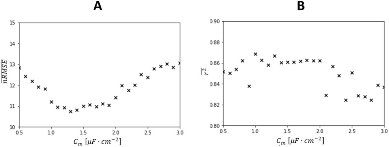
Sensitivity analysis on parameter C_m for the dataset DTA₃₅ over [t_r0; t_r3]. The MN size calibration of the N_r MNs was repeated for 0.1μF · cm² increments in the value of C_m. For each increment, the nRMSE and r² values obtained for the N_r calibrated MNs were averaged. The best pair was obtained for C_m = 1.2μF · cm² for the DTA₃₅ dataset.

Specific capacitance at derecruitment

Figure 15 reports for the dataset DTA₃₅ the sensitivity of the LIF-predicted FIDF^sim(t) time-histories to the value of the MN specific capacitance over the time-range [t_r2; t_r5] during which the MUs are being derecruited. In this analysis, the LIF models were scaled with the S_i parameter calibrated in Step (3) and with the C_m parameter value obtained from the sensitivity analysis in Figure 14. In all four datasets, was again parabolic and a global minimum was found for and 2.2μF · cm² for the datasets DTA₃₅, HTA₃₅, HTA₅₀ and HGM₃₀, respectively. In all four datasets, the MN specific capacitance increased during the derecruitment phase as with k ∈ [1.3; 1.7]. These values for the parameter were retained for the final simulations (Figure 12 and Figure 13) over the [t_r3; t_r5] time range.

Figure 15:

Sensitivity analysis on parameter for dataset DTA₃₅ over [t_r2; t_r5]. The LIF-simulations were repeated for the N_r MNs for 0.1μF · cm² increments in the value of C_m. For each increment, the nRMSE and r² values obtained between predicted and experimental FIDFs were averaged. The best pair was obtained for C_m = 1.8μF · cm² for the DTA₃₅ dataset.

MN-driven muscle model

Figure 16 reports for the datasets DTA₃₅ and HTA₃₅, for which the eND_N was the most accurately predicted among the four datasets (Figure 13, Table 3), the time evolutions of the whole muscle force F(t) recorded experimentally (green curve) and the whole muscle forces predicted with the MN-driven muscle model described in Figure 3 using N_r experimental (F_Nr(t), blue curves) and N simulated (F_N(t), red curves) spike trains as inputs. The muscle force trace F_N(t) obtained from the N simulated spike trains derived in steps (1-4) compared with the experimental force F(t) with r² = 0.91 and nRMSE = 15% for the dataset DTA₃₅ and r² = 0.91 and nRMSE = 16% for the dataset HTA₃₅. These results validate the approach provided in this study for predicting the whole muscle force as a collection of MU force contributions from the MN-specific contributions to the effective neural drive. For the dataset DTA₃₅, a high noise in F_N(t) was however predicted during the plateau of force, while the true muscle force was underestimated during the phases of MN (de)recruitment in both cases. The muscle force trace F_N(t) obtained from the N MN spike trains returned more accurate predictions than F_Nr(t) (r² = 0.84 and nRMSE = 27% for the dataset DTA₃₅ and r² = 0.70 and nRMSE = 36% for the dataset DTA₃₅), in which case the reconstruction of the MN pool in steps (1-4) was disregarded and the N_r experimental spike trains were directly used as inputs to the muscle model in Figure 3.

Figure 16:

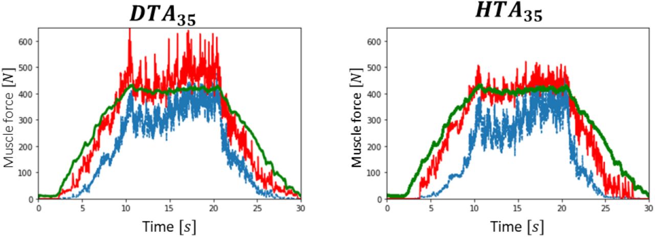
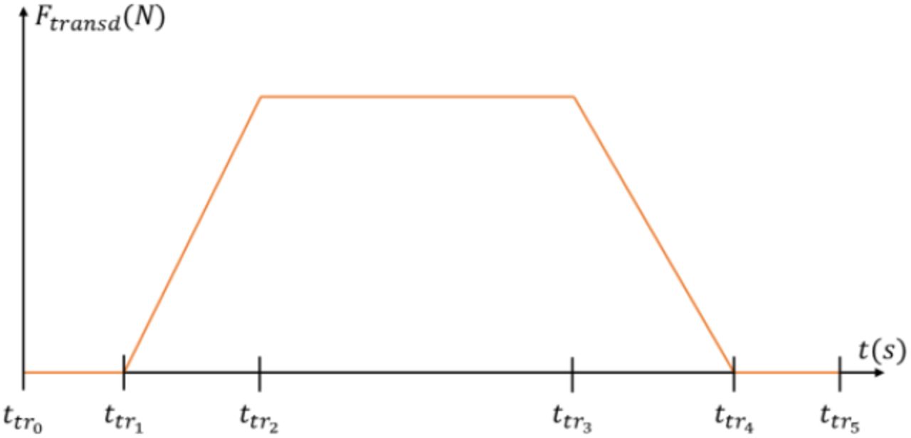
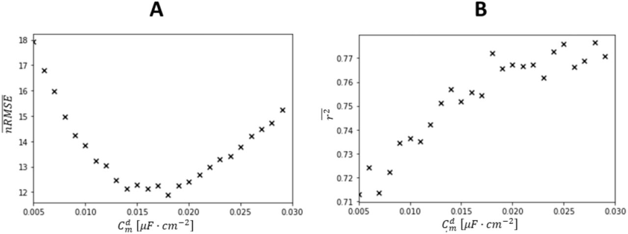
Prediction of the experimental force trace F(t) (green curve) with the MN-driven muscle model described in Figure 3. F_N(t) (blue curve) was predicted with the N_r experimental spike trains input to the muscle model. F_N(t) (red trace) was obtained from the cohort of N experimental spike trains simulated by the four-step approach.

DISCUSSION

This study reports a novel four-step approach, summarized in Figure 1 and displayed in detail in Figure 11, to reconstruct the recruitment and firing behaviour of a complete human pool of N MNs from a sample of N_r experimental spike trains obtained from the decomposition of HDEMG or intramuscular recordings during voluntary contractions. This approach can help neuroscientists, experimentalists, and modelers to investigate MN pool neuromechanics, better understand experimental datasets, and control more detailed neuromuscular models to advance our understanding of the neural strategies taken by the human central nervous system to control voluntary muscle contractions.

The three first steps of our approach identify from a sample of N_r experimental spike trains a distribution of the MN electrophysiological properties across the MN pool. The N_r MN spike trains are used to approximate the common synaptic drive I(t) to the complete MN pool (Figure 7). I(t) is input to a cohort of N_r LIF models. The LIF firing behaviour is entirely described by the MN Inert Period parameter IP_i, derived from the experimental data (Figure 8), and by the MN size S_i parameter to which all the MN electrophysiological properties are related, according to the relations provided by Caillet et al. (2021). After calibration of the S_i parameter, the N_r LIF models accurately mimic the filtered discharge behaviour and accurately predict the recruitment dynamics of the N_r experimental MNs (Figure 9). The N_r MNs are allocated into the complete MN pool (Figure 5B and C) according to their recorded force recruitment thresholds (Figure 4B) and a typical species- and muscle-specific F^th(j) distribution (Figure 5). From the previous findings, the continuous distribution of MN sizes S(j) (Figure 10A) is derived for the complete pool of N MNs. S(j) defines the electrophysiological properties (Caillet et al., 2021) of the MNs constituting the complete MN pool. The neural behaviour of the complete pool of N MNs is predicted in the 4^th step with a cohort of N S_j-IP_j-scaled LIF models and the application of the common synaptic drive I(t) (Figure 10).

Validation of the approach

The approach was successfully validated both for individual MNs and for the complete pool of N MNs. By blindly scaling the LIF models in steps (1-3) with permutations of N_r – 1 input experimental spike trains, the filtered discharge behaviour and the recruitment dynamics of the N_r individual MNs were accurately predicted for the four investigated datasets (Figure 12). The effective neural drive (eND_N) to muscle elicited by the complete pool of N MNs was also accurately predicted by the 4-step approach for the HTA₃₅, DTA₃₅ and HGM₃₀ datasets (Figure 13, Table 3). The latter result suggests that the recruitment dynamics and the normalized distribution of firing rates across the firing MN pool were accurately predicted for the non-identified population of N – N_r MNs.

The intermediary predictions output by the MN pool model are besides consistent with other findings from the literature and suggest that the four-step approach realistically describes the true MN pool neurophysiology and dynamics. For example, while the MN size parameter calibration (Figure 9) only relies on the minimization of the root-mean square difference between experimental and predicted FIDFs, the normalized time-history of the FIDFs (high r² in Figure 12) and the MN recruitment times (low Δft¹ values in Figure 12) of the N_r MNs are both accurately mimicked (Figure 9) and blindly predicted (Figure 12) for all four datasets. The S(j) distribution obtained from the LIF calibrations in step (3) is besides consistent with the mathematical relationship existing between rheobase and MN size (Caillet et al., 2021), which was not used in the current approach. The distribution in rheobase (Figure 7A) and of MN size (Figure 10A) yield . Considering that , this relation respectively yields for the smallest and largest MNs and , which are consistent with the relationship I_th = 3.8 · 10⁸ · S^2.5 that was obtained from an extensive literature meta-analysis by Caillet et al. (2021). The range of MN surface areas [0.15; 0.36]mm² and input resistances [0.5; 4.1]MΩ obtained from the S(j) distribution falls into the classic range of MN properties for cats (Manuel et al., 2019; Caillet et al., 2021), which is consistent with the distribution of rheobase values used in Step (2) that was obtained from cat data. The distribution of MN input resistance in the MN pool, obtained from the calibrated sizes S(j), defines the individual MN rheobase thresholds and predicts that 85% of the human TA MU pool is recruited at 35%MVC (Figure 10C), which is consistent with previous findings in the literature (Van Cutsem, M. et al., 1997; Heckman & Enoka, 2012).

Added value of the approach

The workflow provides a method to support future experimental investigations and better understand datasets of N_r experimental spike trains obtained from signal decomposition. HDEMG decomposition techniques commonly identify samples of few tens of MNs (Del Vecchio et al., 2020) at most, i.e. typically less than 10% of the MU pool. The signal decomposition process can be refined and more MNs can be identified by iteratively running this workflow and using the N – N_r simulated spike trains of the non-identified MNs as a model for identifying more MNs from the recorded signals. The method identifies credible MN-specific electrophysiological and morphometric properties, including MN membrane surface area, input resistance, capacitance, rheobase and time constant, for the dataset of N_r experimental MNs and for the N – N_r MNs that cannot be recorded. The method also provides two-parameter scaled LIF models described in step (3) to accurately replicate the recruitment and firing behaviour of the N_r identified MNs (Figure 9). This method shows in Figure 5, Figure 10A and Table 2, that the N_r-sized samples of MNs currently identified from HDEMG decomposition are not representative of the complete MN pool, as demonstrated by the [0.65; 0.80] coher_Nr values in Table 2, and provides the eND_N computed from the N simulated MN spike trains of the complete MN population to tackle this limitation. EMG decomposition shows a bias towards identifying large high-threshold MUs because of their larger electric signal amplitude detected by the HDEMG electrodes. Consequently, the CST_Nr computed from the N_r identified MNs is not an accurate representation of the true eND (Figure 13, Table 3). During the force ramps in [t₁; t₂] and [t₃; t₄] (Figure 2), where the eND_Nr can reach 70% nME, the eND_N is accurately estimated because it includes the firing activity of the complete fraction of the smaller MNs that were underrepresented in the experimental dataset. The eND_N besides includes the complete population of high-threshold MNs, which reduces noise (orange vs blue trace in Figure 13) during the plateau of force in [t₂; t₃]. The eND_N also filters the local non-physiological variations displayed by the eND_Nr such as the decrease in eND_Nr in [10; 15]s in DTA₃₅ and HTA₃₅ (top plots in Figure 13), the sudden rise and drop in eND_Nr at t = 10s and t = 23s in HTA₅₀ (bottom left plot in Figure 13) or the steeply decreasing eND_Nr from t = 28s in HGM₃₀ (bottom right plot in Figure 13). Understanding these limitations has important implications in neuromuscular modelling when the CST_Nr is input to a muscle model as a unique neural control (Sartori 2017, Kapelner 2020, Thompson 2018).

As it relies on a physiologically realistic description of the MN neurophysiology, this validated method is a tool for testing neurophysiological hypotheses and investigating some mechanisms and properties of the complete MN pool that cannot be directly observed experimentally in conditions of human voluntary contractions. The sensitivity analysis in Figure 14 reveals that the membrane specific capacitance C_m, which cannot be measured in humans, equals to 1.2 μF · m⁻² in human hindlimb muscles, which is consistent with previous findings in mammals (Gentet et al., 2000). According to the sensitivity analysis in Figure 15, the mechanisms that lead the MNs to discharge at relatively lower firing rates at derecruitment than at recruitment (Figure 4C) can be explained by an increase of the MN membrane specific capacitance by a factor in [1.3; 1.7] when MNs are derecruited. As the S, C, R, τ parameters of the LIF models cannot be directly measured in humans (Manuel et al., 2019), and considering that the normalized mathematical relationships relating the MN electrophysiological parameters can be extrapolated to humans (Caillet et al., 2021), the four-step approach is an adequate framework to test hypotheses on the scalability of these MN electrophysiological properties between mammals and humans and to estimate typical human-specific ranges of absolute values for these properties.

This four-step approach advances the state-of-the-art in MN pool modelling. As discussed in the introduction, using a sample of N_r experimental MN spike trains permits for the first time in human MN pool modelling to (1) estimate the true time-course of the common synaptic input to the MN pool, which cannot be measured experimentally, (2) evaluate with a one-parameter calibration, available HDEMG data and knowledge from the literature, the MN-specific electrophysiological properties of all the MNs in the MN pool and a realistic distribution of these properties across the pool, which could, to date, only be obtained in specialized experimental and MN pool modelling studies in animals (Raikova et al., 2018), and (3) validate the forward predictions of MN spike trains and effective neural drive to muscle to human experimental data. The pool of LIF models, the maximum firing frequency of which is obtained from the available experimental data, intrinsically accounts for the onion skin theory (De Luca, Carlo J. & Hostage, 2010) (Figure 8). It better replicates the MN membrane dynamics of the MN pool than Fuglevand-type phenomenological models (Fuglevand et al., 1993; Carriou et al., 2019), where the MN-specific firing rates are predicted as a linear function of the synaptic input I(t). Moreover, LIF models credibly replicate most of the MN membrane dynamics (Teeter et al., 2018) and allow accurate predictions of the MN pool behaviour (Figure 12, Figure 13), while they provide a simpler modelling approach and a more convenient framework for MN electrophysiological parameter assignment than comprehensive Hodgkin-Huxley-type MN models (Huxley & Niedergerke, 1954; Huxley, 1957; Cisi & Kohn, 2008; Negro & Farina, 2011). As it relies on a physiologically realistic description of the MN pool architecture, the four-step approach is robust to systematic differences in the input experimental datasets. For example, it accurately predicted the individual MN firing behaviour of the N_r MNs for all four datasets (Figure 12) despite the latter being obtained at different levels of muscle contractions, on different subjects and muscles and in different experimental approaches. The approach accurately predicted the eND_N of both DTA₃₅ and HTA₃₅ datasets from N_r = 32 and 21 identified MNs respectively (Table 3), suggesting that the method is not sensitive to the number N_r of identified MNs, providing that the N_r identified MNs and their properties are homogeneously spread in the MN pool, as in datasets DTA₃₅ and HTA₃₅ where at least one MN is identified in the each 10%-range of the rheobase domain. The accurate prediction of eND_N for the dataset HGM₃₀ in the time range [4.7; 7.2]s (Figure 13 bottom-right plot) also suggests that the quality of the predictions is not sensitive to the hindlimb muscle investigated, providing that the F^th distribution is representative of the investigated muscle.

Limitations of the approach and potential improvements

The two validations of the approach (Figure 12 and Figure 13) present some limitations. The local validation in Figure 12 only ensures that the method accurately estimates the MN firing behaviour for the fractions of the MN pool that were experimentally identified. This local validation alone does not inform on the accuracy of the predictions for the non-identified regions of the MN pool and must be coupled with a global validation of the MN pool behaviour by validating the predicted eND_N. While the local validation was successful for the HTA₅₀ dataset (Figure 12), where less than 30% of the active MN pool is represented, it is inferred in Figure 13C that the individual MN firing rates were overestimated for the first half of the non-recorded MN pool. This local validation would be self-sufficient for experimental samples that contain a large and homogeneously spread population of identified MNs, obtained from decomposed fine-wire intramuscular electrode and HDEMG grid signals. The validation of the eND_N is performed in this study against an experimental force recorded by a transducer (green traces in Figure 13), which accounts for the force-generating activity of both the muscle of interest and the synergistic and antagonistic muscles crossing the ankle. The experimental force trace measured in the TA datasets may be an acceptable validation metric as the TA muscle is expected to explain most of the recorded ankle torque in dorsiflexion. The TA muscle is indeed the main dorsiflexor muscle with a muscle volume and maximum isometric force larger than the flexor hallucis longus muscle, which moment arm is besides not aligned with the dorsiflexion direction and mainly acts for ankle inversion. However, the gastrocnemius lateralis, soleus, and peroneus muscles acts synergistically with the GM muscle for ankle plantarflexion and the experimental torque recorded in dataset HGM₃₀ may not be representative of the GM muscle force-generation activity and may not be a suitable validation metric for eND_N. In Figure 13, the decreasing eND_N and eND_Nr (orange and blue dotted traces) may accurately describe a gradually increasing sharing of the ankle torque between synergistic muscles initially taken by the GM muscle, which the constant validation trace does not capture. To answer such limitations, the predicted eND_N should be validated against a direct measure of muscle force, which can be performed as in other recent studies (Dick et al., 2017; Martinez-Valdes et al., 2021; Waasdorp et al., 2021) with ultrasound measurements of the muscle fascicle or of the muscle tendon concurrently obtained with (HD)EMG recordings of the muscle activity.

While the method predicts a list of simulated spike trains and a eND_N that more accurately describes the MN pool behaviour than the experimental and eND_Nr, as discussed previously, the accuracy of these predictions (Figure 12 and Figure 13) remains sensitive to the distribution in the entire MN pool of the N_r MNs identified experimentally, reported in the third column of Table 2. Because of the definition of the synaptic current input I(t), the eND_N onset is defined by the recruitment time of the lowest-threshold MN N₁ identified experimentally, as shown in Figure 13, while the unknown firing behaviour for of the non-identified MNs of rheobase lower than is not captured. This is not an issue in samples of homogeneously distributed MNs like dataset DTA₃₅, where the 16^th smallest MN (first 4% of the pool of threshold-increasing MNs) is identified (Figure 5BC), Table 2) and the eND obtained from the 15 first MNs is not predicted during the short time range [2.1,2.3]s, where the whole muscle builds only 1%MVC (top-left plot in Figure 13). However in heterogeneous or incomplete samples like dataset HTA₅₀ the lowest-threshold (232^nd, Table 2) identified MN identified is recruited at and the approach wrongly returns a zero muscle neural drive eND = 0 for the time period [1.6; 6.1]s where the muscle actually builds 20%MVC during the ramp of contraction (bottom-left plot in Figure 13). To tackle this issue, the normalized force trace, which is non-zero for and representative of the CSI in this time region, could be scaled to consistent values of synaptic current and used in lieu of the current definition of I(t). Such synaptic input would also be more physiologically representative of the true synaptic current than I(t), which coher_Nr value is below 1. However, this approach, which may not be suitable for non-isometric conditions, is not applicable in forward predictions of unknown whole muscle force from neural inputs. In pre-defined protocols of muscle contractions like trapezoidal ramps (Figure 2), the region could also be extrapolated by regression. Experimental samples of homogeneously distributed MNs are also required to derive realistic S(j) and IP(j) distributions with the four-step approach. As observed in Figure 12, ignoring in the derivation of I(t), IP(j) and S(j) the spike trains of the MNs that are representative of a large subset of the MN pool affects the accuracy of the predicted recruitment and firing behaviour of the MNs falling in that subset (Figure 12). More specifically, the non-physiological distribution IP(j)[s] = 5.6 · 10^-4 · j^0.80 was fitted to the experimental data of the 14 high-threshold MNs identified in dataset HTA₅₀, where the neural information of the 60% smallest MNs of the MN pool (Table 2) is lacking. Such IP(j) distribution overestimates the LIF-predicted maximum firing frequency of low-threshold MNs, which explains the overestimation of the eND_N in Figure 13 (bottom-left plot, orange curve). Non-physiological predictions can be avoided by adding artificial data points consistent with other experiments or with the literature in the rheobase regions of the MN pool where no MNs were experimentally identified. For example, using an IP(j) relationship consistent with a dataset of homogeneously distributed MNs (DTA₃₅) constrained the predicted maximum firing rates to physiological values and returned more accurate predictions of the eND_N (bottom-left plot, purple curve).

The four-step approach presents the following limitations and simplifications which make it currently unfeasible to mimic and predict certain neural mechanisms. First, it is inferred from the calibrated FIDFs in the [t_tr1; t_tr2] regions (Figure 9A) that the MN firing behaviour could be better predicted if the LIF IDF – I gain was lower for all MNs for large input currents. In LIF models, the IDF – I gain is mainly determined by the MN membrane capacitance C = C_m · S, tuned by parameter calibration and sensitivity analysis in this study. To achieve a lower gain, a nonlinear 1^st-order LIF model, a 2^nd-order LIF model, a time-history-dependent C parameter or a 3-parameter LIF model are options. However, considering the overall accurate predictions of the MN firing behaviours (Figure 12), its low computational cost and its modelling simplicity, the LIF model defined in this study was considered an adequate trade-off between accuracy and complexity and no other modelling approaches were pursued. A second limitation of the study is that, as discussed previously, the LIF parameters are tuned with typical cat data (Caillet et al. 2021) while the experimental MN spike trains were obtained from humans. While the normalized mathematical relationships relating the MN electrophysiological parameters of the LIF model (R, C,τ,ΔV_th) can be extrapolated between mammals (Caillet et al. 2021) and thus to humans, no experimental data is yet available to scale these relationships to typical human data. A further limitation is that, in its current form, the method disregards the synaptic noise SN(t) specific to each MN and the inter-spike variability (ISV). The synaptic current I(t) is simplified as the common synaptic drive to the MN pool. Considering that the MN pool and the MU neuromechanical mechanisms are expected to filter the MN-specific SN(t), this simplification is adequate for accurate predictions of the eND_N and of the whole muscle force (Farina, 2015). Sometimes modelled as a random Gaussian-like event (Fuglevand 1993), the ISV can be obtained as the response to a SN(t) white noise added to the current definition of the synaptic current as I(t) = CSI(t) + SN(t). The relative proportion of CSI and SN in % of the variance of the total synaptic current can be approximated from Figure 2A in Negro et al. (2016). Accounting for SN(t) might improve the accuracy of the predicted firing behaviour of the largest MNs, for which the largest Δft¹ and nRMSE and lowest r² values were obtained in Figure 12 for all four datasets. These MNs are recruited at a rheobase close to the nearly constant common synaptic current I_plat maintained during the plateau of force in the time range [t_tr2; t_tr3 ≈ (I_th ≈ I_plat) and their firing behaviour and recruitment dynamics are dominantly dictated by random fluctuations of SN(t). The capacity of the synaptic drive to generate larger synaptic currents I(t) in larger MNs (Heckman 2012) could be accounted for with a MN size-specific scaling factor assigned to the I(t) trace obtained in Figure 7 (B). The MN-specific decrease in current threshold between recruitment and derecruitment phases shows a MN-specific random behaviour around a global linear tendency across the complete MN pool (Figure 4B), which could be captured by adding a randomized component to the value of the MN input resistance which is increased between recruitment and derecruitment phases (see Methods). Such an approach would better predict the derecruitment times of individual MNs and the derecruitment time period of the predicted eND_N.

An additional limitation is that the typical F^th(j) and I_th(j) threshold distributions, derived for mapping the N_r identified MNs to the complete MN pool (Figure 5) and for scaling the CSI to physiological values of I(t) (Figure 7), were obtained from studies which relied on experimental samples of MN populations of small size. These source studies therefore did not ensure that the largest and lowest values were identified and reported, and that the identification process was not biased towards a specific subset of the MN pool, such as larger MNs. In such cases, the true threshold distributions would be more skewed and spread over a larger range of values, as discussed in Caillet et al. (2021), than the distributions reported in Figure 5 and Figure 7. The F^th(j) distribution is besides muscle-specific (Heckman 2012) with large hindlimb muscles being for example recruited over a larger range of MVC than hand muscles. However, enough data is reported in the literature to build the F^th(j) distributions for the TA and first dorsal interossei human muscles only. MN rheobase cannot be recorded in humans and the I_th(j) distribution in Figure 7A was obtained from cat experimental data obtained from various hindlimb muscles. For these limitations, the two first steps of this approach could be made subject-species- and muscle-specific by calibrating the F^th(j) and I^th(j) described as the 3-parameter power functions defined in this study.

Relevance for neuromuscular modelling

In this study, a MN-driven muscle model of in-parallel Hill-type actuators describing the MUs (Figure 3) is used to perform forward predictions of the whole muscle force in voluntary isometric contraction. Each Hill-type actuator predicts the excitation, activation and contraction dynamics of each MU constituting the muscle, i.e. the MU neural, action potential, calcium transient, activation and contraction behaviour. The whole muscle force is computed as the linear summation of the predicted MU forces. The MN-driven muscle model either takes as inputs the N_r individual MN spike trains identified experimentally (blue trace in Figure 16) or the N simulated spike trains (red trace in Figure 16).

This approach advances the state-of-the-art in neuromusculoskeletal modelling on several aspects. The MN-driven muscle model (Figure 3) is driven by an input vector of experimental MN spike trains, so extending the classic single input EMG-driven approach, in which the individual MN contributions are lumped into a unique neural control to the muscle, taken as the rectified-normalized-filtered envelope of recorded bipolar EMGs (bEMGs) (Hof & Van den Berg, 1981; Zajac Felix, 1989; Lloyd & Besier, 2003). bEMGs are also challenging to interpret (De Luca, Carlo J., 1997) and come with intrinsic experimental limitations that are circumvented by HDEMG and/or intramuscular approaches (Staudenmann et al., 2006; Mesin et al., 2009; Varrecchia et al., 2021), for which current decomposition techniques are a reliable process across operators (Hug, Avrillon et al., 2021). The MN-driven muscle model (Figure 3) also represents an improvement with respect to recent studies which merged the individual MN spike trains obtained from decomposed HDEMG or intramuscular recordings into a unique neural control, the CST_Nr, given as input to Hill-type (Sartori et al., 2017; Kapelner et al., 2020) and twitch-type (Thompson et al., 2018) muscle models. As in bEMG-driven approaches, the CST_Nr loses the MN-specific information of MN neural behaviour, recruitment dynamics and contributions to the neural drive. The multi-MU model in Figure 3 expands the classic multiscale approach of modelling a whole muscle as a single equivalent sarcomere or MU (Zajac Felix, 1989). Such multiscale models usually (1) cannot explicitly model the dynamics of MU recruitment, (2) disregard the continuous distribution of MU properties in the MU pool that typically affects the MN firing behaviour (Caillet et al., 2021), the calcium dynamics in the sarcolemma (Baylor & Hollingworth, 2003), the cross-bridge cycling dynamics (Rockenfeller & Günther, 2018), the force-velocity relationship (Alcazar et al., 2019) and the MU maximum isometric force distribution, and (3) cannot account for the passive properties of the intramuscular matrix of passive tissues (Herzog, 2019). Despite relevant modelling work in multi-scale modelling (Hatze, 1977; Hatze, 1980; Dorgan & O’Malley, 1997; Song et al., 2008; Dick et al., 2017; Hussein et al., 2021), multi-MU muscle models like the one proposed in Figure 3 provide a more convenient framework to answer the above limitations. The multi-MU models available in the literature (Hatze, 1980; Legreneur et al., 1996; Callahan et al., 2013; Hamouda et al., 2016; Potvin & Fuglevand, 2017; Raikova et al., 2018; Carriou et al., 2019) were however never assessed with experimental neural inputs or validated against synchronously recorded experimental data, and simply recreated the recruitment and firing MN-specific behaviour of the modelled individual MUs, which are intrinsic to the experimental sample of N_r spike trains obtained from signal decomposition. The MN-driven multi-MU muscle model in Figure 3 therefore diverges from past approaches by predicting and experimentally validating the whole muscle force using a physiologically realistic model of a MU population receiving an experimental MN spike trains as a vector of inputs.

The N-MU model, that receives as inputs the N spike trains generated by the four-step approach, predicted the whole muscle force more accurately (Table 3) than the N_r-MU model receiving the N_r individual MN spike trains (Figure 16). As discussed previously, the N_r identified MNs are not representative of the distribution of MN and MU properties in MU pool (Figure 5) and of the neural activity of the complete MN pool (Figure 13). In neuromuscular modelling, this affects the realistic assignment of MU properties, such as MU type and MU maximum isometric force, to the sample of N_r MUs and limits the interpretations of the N_r-MU muscle model predictions. The N_r-MU model besides underestimates the whole muscle in the regions of low muscle activity where dominantly low-threshold MUs are recruited but are under-represented in the experimental sample. A similar limitation arises for the studies using the CST_Nr as input to their muscle models. Describing the complete population of MUs and accounting for the whole distribution of MU neuromechanical properties in the muscle with the N-MU model tackles the limitations related to the N_r-MU model. A few other studies have predicted whole muscle forces with a collection of N MU Hill-type (Legreneur et al., 1996; Callahan et al., 2013) Hill-Huxley-type (Carriou et al., 2019) or twitch-type (Raikova et al., 2018) muscle models from the neuromuscular activity of complete pools of MUs, the MN firing behaviour and recruitment dynamics of which were modelled with the Fuglevand’s formalism. Contrary to these studies which considered an artificial synaptic input and performed indirect validations of the predicted forces against results from other models, the whole muscle force predictions in Figure 13 and Figure 16 were obtained from and validated against experimental data. The N-MU model besides receives the N validated neural inputs from the four-step approach that is more realistic and advanced than the Fuglevand’s formalism, as discussed previously.

The N-MU neuromuscular model defined in this study relies on realistic and mechanistic descriptions of the MU-specific neural and mechanical mechanisms and on physiological parameters that can be interpreted and measured experimentally in mammals. The isometric muscle force trace can therefore be accurately predicted in this approach without relying on any parameter calibration except the MN size in step 3. The neuromuscular model proposed in this study is thus more suitable for investigating the muscle neuromechanics and confidently reconciling spinal motor control and muscle contraction than typical EMG-driven models, the neural parameters of which do not have a direct physiological correspondence and must be calibrated to match experimental joint torques (Lloyd & Besier, 2003; Sartori et al., 2012; Pizzolato et al., 2015).

ACKNOWLEDGEMENTS

AC was supported by the Skempton Scholarship and LM by an Imperial College Research Fellowship granted by Imperial College London.

Footnotes

• CONFLICT OF INTEREST STATEMENT: The authors declare no competing financial interests.