

Abstract
Neural network models have been instrumental in revealing the foundational principles of whole-brain dynamics. Here we describe a new whole-cortex model of mouse resting-state fMRI (rsfMRI) activity. Our model implements neural input-output nonlinearities and excitatory-inhibitory interactions within areas, as well as a directed connectome obtained with viral tracing to model interareal connections. Our model makes novel predictions about the dynamic organization of rsfMRI activity on a fast scale of seconds, and explains its relationship with the underlying axonal connectivity. Specifically, the simulated rsfMRI activity exhibits rich attractor dynamics, with multiple stationary and oscillatory attractors. Guided by these theoretical predictions, we find that empirical mouse rsfMRI time series exhibit analogous signatures of attractor dynamics, and that model attractors recapitulate the topographical organization and temporal structure of empirical rsfMRI co-activation patterns (CAPs). The richness and complexity of attractor dynamics, as well as its ability to explain CAPs, are lost when the directionality of underlying axonal connectivity is neglected. Finally, complexity of fast dynamics on the scale of seconds was maximal for the values of inter-hemispheric axonal connectivity strength and of inter-areal connectivity sparsity measured in real anatomical mouse data.
Introduction
Whole brain resting state fMRI (rsfMRI) has been widely used to map functional organization of spontaneous large-scale activity in the human brain [1-3]. These measures have been paralleled and informed by computational models of large-scale interactions between areas of the brain. Such network models typically incorporate anatomical connections as inferred by diffusion tensor imaging, and are used to understand and predict the principles and mechanisms of the ensuing collective neuronal dynamics [4-7]. Computational models have first been employed to describe steady-state measures of functional connectivity averaged over many minutes of resting state activity [8-12], and more recently to characterize dynamical changes in network configuration occurring on the time scale of tens of seconds [13-17].
In recent years, studies of rsfMRI in humans have begun to be complemented by similar measures performed in preclinical species, including rodents. Mouse rsfMRI studies are emerging as important tools to understand the mechanisms and principles of resting state large scale brain activity because they can be accompanied by genetic manipulations and causal interventions aimed to mimic pathologies [18-20]. The use of physiologically accessible species can also crucially allow a more precise measure of the underlying axonal connectivity and its directionality [21-23], which cannot at present be estimated in humans with Diffusion Tensor Imaging (DTI), as this technique lacks information on fiber directionality, and does not allow to reliably resolve long axonal tracts [24]. rsfMRI studies in mice have revealed important principles in the organization of neuronal activity, such as the formation of large-scale functional hubs and the relationship between the mouse axonal connectome and its functional connectivity [21,25-27]. Importantly, they have revealed a rich dynamics in mouse rsfMRI time series [28,29], which partly recapitulates that seen in humans [30-33] and that is governed by a few dominant co-activation patterns of synchronous fMRI activity across areas on a time scale of seconds, termed fMRI co-activation patterns (CAPs) [33,34].
Because of the growing importance of rsfMRI studies in the mouse, theoretical research has begun to extend to network models of large-scale rodent brain activity [35-38]. These models of the mouse brain can help resolving many of the still unknown complex neurophysiological processes and principles that shape spontaneous rsfMRI activity in the mammalian brain. For example, we know little about the mechanisms and neural principles leading to the emergence and significance of the infraslow fMRI CAPs. Addressing this issue also from a computational standpoint is of crucial importance given the emerging contribution of these fluctuating patterns in shaping rsfMRI dynamics in human and animals, and also the numerous and conflicting theories related to their origin and relationship with underlying cortico-cortical connectivity or modulatory input [28,29,39-41]. Importantly, mouse brain models can also crucially complement those in humans because the high resolution directed connectomes in this species [23] allows to address the role of fiber directionality in contributing to brain dynamics, something which is elusive with human brain modeling.
To fill this knowledge gap, here we developed a whole-cortex neural network model that combines realistic directional anatomical connectivity of the mouse neocortex [21,22,42] with simple non-linear firing rate dynamics in each area. The model allows to simulate emergent neuronal phenomena elicited by the collective dynamics of the interconnected brain regions. We first fitted the model parameters to match the time-averaged pattern of relative activation across areas and the time-averaged (static) functional connectivity matrix. Departing from prior models, we next used our ability to study in detail the moment-to-moment dynamics of these networks to make several novel predictions about the seconds-scale dynamics of the whole-cortex rsfMRI recordings and its relationship with the underlying anatomy of inter-areal connections. Specifically, we succeeded in computing the attractor dynamics generated by the model, revealing a rich structure of oscillatory and stationary attractors. Importantly, computational analysis of real-world empirical rsfMRI data revealed that analogous signatures of attractor dynamics are present in real data. We also found that features of real CAPs seen in mice can be explained by the model attractor dynamics, but only when considering directed structural connectivity. The richness and complexity of attractor dynamics was maximal for values of the inter-hemispheric connection strength and of inter-areal connectivity sparsity found in real anatomical mouse data.
2 Results
We designed a novel large-scale neural network model of the whole mouse cortex and tested its predictive value. The model was endowed with a directed matrix of the structural connectivity between cortical areas taken from mouse data, generating neural and rsfMRI dynamics of each area that are biologically plausible, yet simple enough to allow for a thorough numerical and analytical study of their dynamics. The model parameters were selected to fit “static” (i.e. averaged over time scales of minutes) rsfMRI activity and functional connectivity of real mouse data. The model was then used to make novel predictions about the role of specific elements of the structural connectivity in generating whole-cortex attractor dynamics. These model predictions were tested on real mouse rsfMRI time series by comparing the predictions against “dynamic” (i.e. defined on faster time scales of one or few seconds) features of rsfMRI functional connectivity such as CAPs.
2.1 Fitting a large-scale neural model of mouse cortex to time-averaged activity and functional connectivity of rsfMRI data
We designed a large-scale neural network model (Fig. 1A) including 34 cortical areas of the mouse brain (17 per hemisphere). The chosen number of areas allowed us to study attractor dynamics with state-of-the art numerical techniques [43] and reduce rsfMRI data overfitting by the model. Each area was modelled to comprise one excitatory (E) and one inhibitory (I) mutually interacting neural populations. Each population was described as a threshold logic unit [44-46] whose states, representing the spiking activity of each cortical area, were updated synchronously at discrete time steps. The total input to each excitatory population included excitatory and inhibitory activity from the same area, and the excitatory activity from other cortical areas, weighted with the structural connectivity matrix. The total input terms to each inhibitory population included instead inhibition and excitation from the same area. Further, a noise term was added as input to both inhibitory and excitatory neurons, to express the net effect of stochastic components of neural activity.

A) Our model incorporates 34 (17 per hemisphere) cortical areas (listed on the left), each with an excitatory (E) and an inhibitory (I) population. The excitatory populations are connected to each other through a structural connectivity matrix taken from the mouse connectome (multiplied by a global scaling coefficient GE,E), and are also connected locally to the corresponding inhibitory population.
B) Mathematical model that describes the temporal evolution of the spiking activity in each area. In each population, the incoming synaptic weights are multiplied by the presynaptic activities, to produce the total postsynaptic current. In turn, this current is summed to a noise term and passed through a threshold-based activation function, to produce a binary activity: 0 if the cortical population is silent, and 1 if it is firing. We derived the rsfMRI signal from each area as the total postsynaptic current of the corresponding excitatory population.
The cortico-cortical structural connectivity inserted in the model was derived by the mouse axonal connectome [23] by estimating the number of connections from the entire cortical source region to the unit volume of the cortical target region [21,22,47]. The structural connectivity was multiplied by a global scaling factor (a free parameter determined by best fit which was the same for all the connections in the model), which represents the average synaptic efficacy per unit of structural connectivity strength. In keeping with previous investigations, inter-areal E to E connectivity within and across hemispheres was assumed to be symmetric across the sagittal plane – that is, the R to R and R to L connections originating from the R hemisphere are respectively identical to the L to L and L to R connections originating from the L hemisphere [21,23,47]. rsfMRI BOLD activity in each area resulting from the underlying neural activity was modeled as the total input current to the excitatory population in each area (Fig. 1B). This assumption is supported by the finding that BOLD correlates best with the local field potential (LFP) [48,49], and that the LFP reflects the synaptic inputs to excitatory neurons [48,50].
The free parameters of our network model were the global scaling coefficient of the structural connectivity (GE,E), the strength of the I to E, E to I and I to I connections (JE,I, JI,E, JI,I, respectively), the membrane potential firing threshold (Vthr), and the standard deviation of the noise sources (σ). We chose the values of these parameters so that they provided the best fit of the time-averaged mean of the rsfMRI signal in each area and the subject-averaged cross correlation (termed Functional Connectivity, FC) between all pairs of areas that were computed from the experimental mouse data (see Methods, SubSec. 4.5). We report the best-fit values of these parameters in Tab. S1.
The experimental rsfMRI data used for model fitting and model validation were collected from 15 C57BL/6J wild type mice in the same 34 cortical regions used for the axonal connectome [21] (Fig. 1A).
To test how well our model reproduced empirical rsfMRI time series, we first compared the values of the time-averaged rsfMRI activity in the model (Fig. 2A) and in the empirical data (Fig. 2B). The pattern across areas of rsfMRI activity of the model reproduced remarkably well that of the data (ρ = 0.85, p < 10−5). Importantly, the model also closely reproduced two hallmark features of rsfMRI organization in the mouse brain, namely a highly synchronous rsfMRI activity within the Default Mode Network (DMN) and the Lateral Cortical Network (LCN) [42] and the presence of a robust inter-hemispheric homotopicity exemplified by the symmetry of the time-averaged rsfMRI activity between left and right hemispheres [51].

A) Relative across-area distribution of the time-averaged rsfMRI predicted by the model. For this calculation, the time-averaged rsfMRI values were normalized between −1 and +1 as explained in Methods.
B) As in A, but obtained from the empirical mouse rsfMRI data.
C) Relative across-area distribution of the time-averaged spiking activity of the model.
D) Static FC matrix of model rsfMRI time series.
E) Static FC matrix of the empirical mouse rsfMRI data.
F) Comparison between the probability distributions of the values of the entries of the FC matrices, obtained from panels D, E.
G) Model FC matrix between the regions in the right hemisphere with the highest average resting state mean activity. To highlight the most functionally connected areas, the FC matrix was thresholded to 0.6 of the maximum off-diagonal entry.
H) As in G, but for the empirical FC matrix. In panels G, H, for simplicity, we showed only the reduced FC matrices in the right hemisphere, while the same results are obtained for the left hemisphere.
I) Architecture of the functional subnetwork shown in panel H.
We next considered how well our model reproduced static Functional Connectivity (FC). We found that the topography of the model’s rsfMRI static FC (Fig. 2D) resembles well (ρ = 0.55, p < 10−5) that of the empirical FC (Fig. 2E). Importantly, modelled rsfMRI activity closely reconstituted the actual values of FC of the real data. This was apparent in the probability distribution of FC matrix entries (Fig. 2F) which was remarkably similar between model and real data, with very high overlap of 0.88 between distributions, and almost coincident mean values (0.28 vs 0.27 for the model and the experimental datasets, respectively, p = 0.22, two-sample Welch’s t-test).
To further demonstrate that modelled rsfMRI activity closely reproduced hallmark features of static FC inferred from empirical mouse data, we focused on the FC between the regions showing the highest average resting state mean activity (Figs. 2G, H for model and data, respectively). Our model reconstituted three main cortical subnetworks characterized by higher activity, namely the posterior (VIS, RSP, ACA, PTLp) and anterior DMN (PL, ILA, ORB, AI), and motor areas (MO, SS) belonging to the LCN. This division into subnetworks was further confirmed quantitatively by applying the leading eigenvector method [52] (see SubSec. 4.7) to determine the community structure of the subnetworks. The resulting architecture of the functional subnetworks is schematized in Fig. 2I.
To probe whether the model explained features of the FC that go beyond its similarity with the structural connectivity matrix, following methods reported in [13], we calculated the partial correlation between the theoretical FC matrix of the model and the empirical FC matrix, partialized on their common structural connectivity matrix. We found that the resulting partial correlation values were 0.47 and 0.40 (p < 10−4), when evaluated on the upper and lower triangular parts of the matrices, respectively. This finding implies that our model explains genuine functional interactions among areas, beyond what is simply induced by their common anatomical matrix.
Collectively, these results show that our model closely recapitulates key foundational properties of static cortical rsfMRI activity and connectivity in the mouse brain.
We finally compared the model’s spiking activity with the real and model rsfMRI. We found a very good agreement between interareal patterns of averaged activity (cf. Fig. 2C with Figs. 2A, B): the correlation between the patterns of time-averaged spiking activity and rsfMRI data was ρ = 0.84 (95% CI [0.69, 0.92], p < 10−5) when considering real rsfMRI data and ρ = 0.97 (95% CI [0.95, 0.99], p < 10−5) with modeled rsfMRI time series. The Pearson’s correlation between the FC matrix of spiking activity (Fig. S1A) and the FC matrix from empirical rsfMRI data (Fig. 2E) was similarly very robust (ρ = 0.45, p < 10−5) suggesting that spiking activity predicted reasonably well the topography of rsfMRI FC. However, the modeled spiking activity did not reproduce well the average value of empirical FC (0.04 vs 0.27, p < 10−5, Welch’s t-test), a finding consistent with the temporally sparser nature of spiking activity.
2.2 Attractor dynamics in the network model explains rsfMRI co-activation patterns
Prior investigations of empirical rsfMRI time series revealed the formation of time-averaged patterns of functional connectivity such as those described by static resting-state networks, but also uncovered a rich temporal organization of resting-state activity. One prominent feature of this temporal structure is a dynamic reconfiguration, on the timescale of seconds, into transient brain-wide network states, known as rsfMRI co-activation patterns (CAPs), which have been consistently found in both humans [33,53] and mice [28,29]. However, our theoretical understanding of how CAPs emerge and are shaped by the concerted interaction of brain areas at rest remains unclear. To address this question, we thus used our network model to relate CAPs measured from empirical rsfMRI mouse data to the underlying collective dynamics of cortical areas.
In absence of noise, networks tend to evolve into a limited set of patterns of activity, each of which is termed an attractor. It is well known that models of recurrently connected neural networks like the one we employed here exhibit attractor dynamics [45,46,54]. For each attractor, its basin of attraction represents the set of initial activity patterns that eventually end up into that attractor in absence of noise (see Figs. S2A and S2B). In the presence of noise, the dynamics of such networks wanders between attractors. We thus hypothesized that attractor dynamics may also exist in mouse rsfMRI dynamics, and that the emergence and features of CAPs may be related to those of attractors.
To probe this hypothesis, we analyzed the dynamics of our model numerically (see Ref. [43] and Methods, SubSec. 4.8). We found that the spiking activity of our whole-brain model featured transitions, over a few-seconds-timescale, between two kinds of attractors: stationary states and neural oscillations. That is, in the absence of noise, our network converged either to a fixed point where the spiking activity is constant over time (similarly to the Hopfield network [54]), or to a periodic oscillatory sequence of activity patterns. Importantly, our model predicted a one-to-one mapping between the attractors (and their basins) expressed in terms of spiking activity and attractors expressed in terms of rsfMRI activity. This implies that we can show model attractors as patterns of rsfMRI activation, and that evidence of attractors in rsfMRI time series can be taken as evidence of attractors in neural activity dynamics (see SubSec. S3).
Specifically, we found that our network model with the best-fit parameters had 31 stationary states and several thousand oscillatory states (Tab. S2). Our network visited the basins of the stationary attractors for approximately half of the time, and the basins of the oscillatory attractors in the remaining time (Fig. S3C). To illustrate the topography of stationary states, for each of the 31 stationary attractors we computed the mean z-score vectors of the model’s rsfMRI. We report examples of a representative homotopic (#17) and non-homotopic (#13) attractor in Figs. 3A and 3B, respectively.
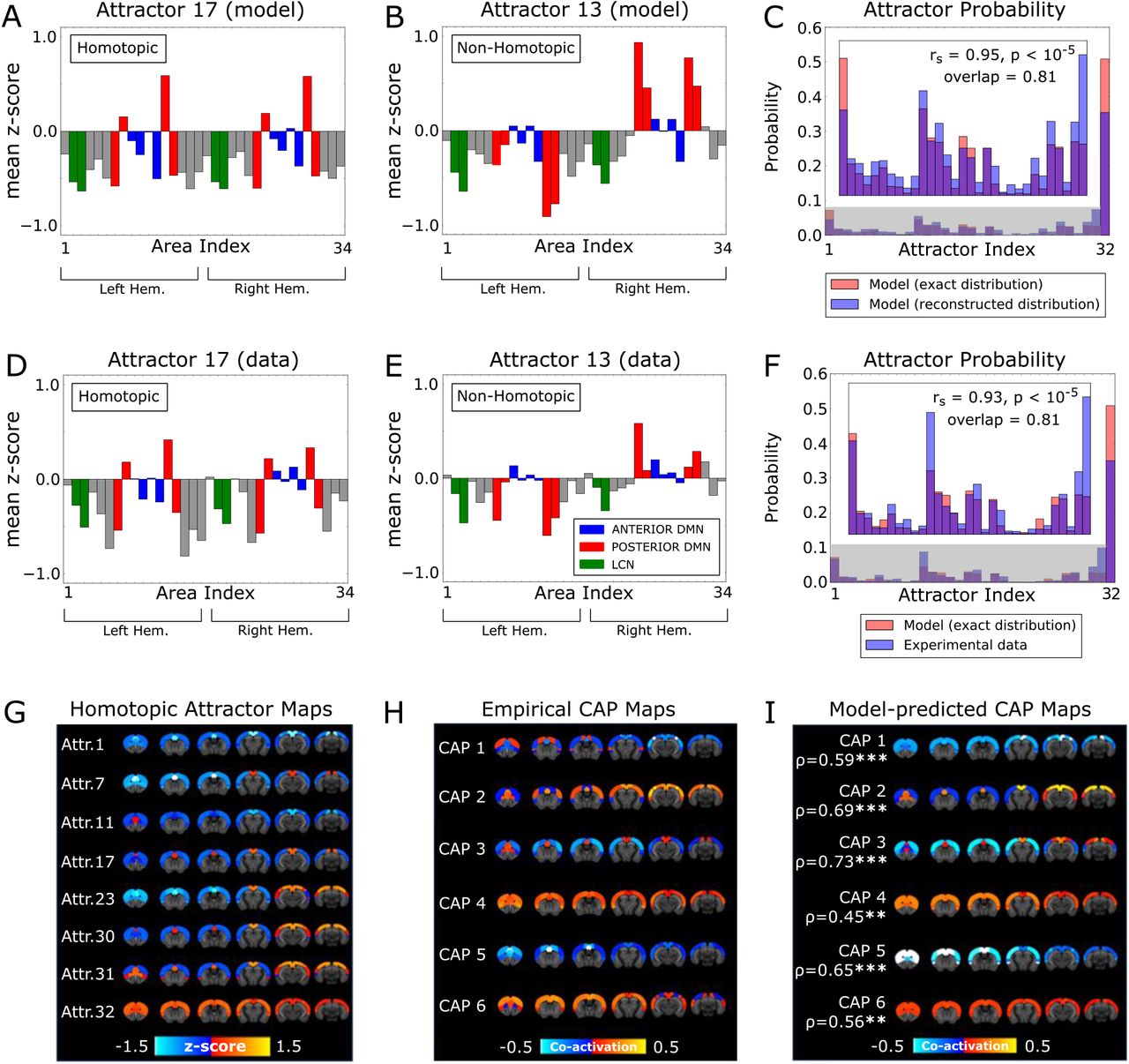
A) Mean z-score vector of model rsfMRI activity classified into an attractor (#17) by the mapping algorithm. This attractor is homotopic.
B) As in A, but for attractor 13. This attractor is non-homotopic.
C) Probability distribution of the basins of attraction, calculated numerically from the spiking activity of the model (red bars), and reconstructed by the mapping algorithm when applied to the model rsfMRI activity (blue bars).
D-E) As in A-B, but in this case the z-scores have been averaged over the empirical rsfMRI states that the mapping algorithm associated to the basins 17 and 13, respectively.
F) As in C, but now the blue bars represent the probability distribution of the basins of attraction reconstructed from the empirical rsfMRI activity.
G) Model-generated rsfMRI activity maps of the neural attractors. In this panel we report only the homotopic attractors, while the non-homotopic attractor pairs are shown in Fig. S3F.
H) CAPs obtained from the empirical rsfMRI time series. Red-yellow indicates co-activation, while blue indicates co-deactivation.
I) CAPs reconstructed from the model attractors and their Pearson’s correlation with the corresponding empirical CAPs.
Interestingly, our model predicted that 7 out of 31 stationary attractors (1, 7, 11, 17, 23, 30, 31, plotted in Fig. 3G) were homotopic, and the remaining stationary attractors were non-homotopic, and occurred in pairs with spatially opposed configurations ((2, 6), (3, 14), (4, 20), (5, 25), (8, 15), (9, 21), (10, 26), (12, 16), (13, 27), (18, 22), (19, 28), (24, 29), plotted in Fig. S3F). The fact that the non-homotopic attractors occurred in pairs of spatially opposed configurations suggests that the average symmetry of rsfMRI activity may actually mask the presence of strong inter-hemispheric asymmetry in moment-to-moment activity. We plotted the probability that each attractor occurred in the model in Fig. 3C (red bars), showing that some attractors (i.e. 1, 11, 12, 13, 16, 17, 19, 27, 28, 30, 31) were far more likely than others.
To understand if empirical rsfMRI time series showed signatures of dynamical attractors similar to those predicted by our model, we developed an algorithm that maps each point of a rsfMRI time series into one of the attractors predicted by the model (see Methods and Figs. S2C,D). By averaging over the rsfMRI time points assigned to each attractor, we could estimate the typical spatial rsfMRI activation pattern of each putative attractor. By counting the number of time points assigned to each attractor, the algorithm next computes the probability with which each attractor is visited over time. Since the probability of each oscillation basin is typically very low (< 10−5 on average), it would be unrealistic to reconstruct them with a limited number of experimental samples. For this reason, we opted to map only the stationary attractors, while we collapsed the basins of the oscillatory attractors into a single macroscopic basin. By comparing the topography of the attractors and the occupation time predicted by the model and estimated from the rsfMRI time series, we could quantify how much the rsfMRI time series were compatible with the given attractor dynamics.
We first validated the performance of the attractor mapping algorithm on the rsfMRI time series simulated from our whole-cortex network model with the best-fit parameters. We found that the mapping algorithm could reconstruct very well the topography of each attractor (mean correlation across all attractors: ρ = 0.94, p < 10−5). Importantly, also the probability distribution of the basins of attraction reconstructed algorithmically from the simulated time series (Fig. 3C, blue bars) matched very well the one computed by the theoretical analysis of the model (Fig. 3C, rs = 0.95, p < 10−5, overlap area 0.81). We next generalized these results by considering degrees of inter-hemispheric connectivity different than the best-fit one. As expected, the mapping algorithm applied to the rsfMRI time series simulated with the model always reconstituted well the attractors computed theoretically by the model itself (Figs. S3A, C). Thus, our empirical attractor mapping algorithm recovers with high precision both the topography and the temporal occurrence probability of the model attractors.
To investigate whether the experimental time series of rsfMRI activity showed a temporal structure compatible with the attractor dynamics of the best-fit network model, we next applied the attractor mapping algorithm to empirical rsfMRI data. When we used the algorithm to map the experimental time series into the attractors of the model with the best-fit parameters, we found that the rsfMRI time series mapped very well into these attractors. Specifically, a comparison of z-score vector plots of empirical rsfMRI signal averaged over all the states the algorithm assigned to basins of attractors 17 and 13 (Figs. 3D, E) with their theoretical counterparts (reported in Figs. 3A, B), revealed a strong similarity, corroborating the goodness of the mapping algorithm (ρ = 0.78, all attractors, p < 10−3, see Fig. S3D). The probability of time occupancy of the basins of attraction estimated from real data also matched remarkably well that obtained from a theoretical analysis of the best-fit model (rs= 0.93, p < 10−5, overlap area, 0.81, Fig. 3F). These results show that the experimental rsfMRI time series are compatible with a structure of attractor dynamics similar to the one generated by our best-fit model.
Importantly, the match between empirical rsfMRI time series and the model’s attractor structure was maximal when comparing the empirical data with the model attractors specifically produced when using as model parameters those determined by best fit of the time-averaged activity and functional connectivity. Computing this match with a different set of model parameter values produced a weaker match between rsfMRI and model attractors (Fig. S3C). Thus, the second-scale dynamics of the empirical rsfMRI time series is compatible with attractor dynamics of the specific form generated by the best-fit model, despite the parameters of our model not being optimized to fit seconds-scale dynamics.
We next asked whether the model’s attractor dynamics could explain the emergence of CAPs in real data. For each time frame of empirical mouse rsfMRI activity, we compared the CAP it was assigned to (by the empirical clustering of the whole brain data done in Ref. [28]) to the cortical model’s attractor it was mapped into (by the attractor mapping algorithm). CAP mapping in the mouse was made by clustering all the whole-brain empirical rsfMRI time series conservatively into 6 different clusters, each representing a recurring pattern of rsfMRI co-activation. Such a relatively small number of different clusters (and thus of different CAPs) was chosen to ensure a high reproducibility of the procedure across datasets [28]. This revealed three distinct CAPs each with a complementary anti-CAP state, i.e. a mirror motif exhibiting a strongly negative spatial similarity to its corresponding CAP (Fig. 3H). Each imaging time frame was mapped to a single CAP and a single attractor. Given that there are more model attractors than empirically determined CAPs, each of the 6 CAPs could potentially capture the contribution of several attractors. We thus reconstructed each CAP from the model’s attractor dynamics as a sum of the spatial activation of each attractor, weighted by the empirical probability that a data point assigned to a CAP was assigned to any given attractor (Fig. S3E). We found an excellent match between empirically determined and model-predicted CAPs, with Pearson’s correlation between the two ranging between 0.45 and 0.73 (p < 10−2) across CAPs (Fig. 3I). This result shows that the attractor dynamics of our model predicts well the topography of empirical CAPs. For each reconstructed CAP, the empirical probability that a data point assigned to a CAP was assigned to any given attractor strongly correlated with the model’s prediction of the probability of occupancy of each basin of attraction (Fig. 3C, 0.61< rs < 0.90, for all CAPs, p < 10−3). Thus, the model predictions of the topography of the attractors and the probability with which the attractors are visited over time allowed us to predict the topography of the empirical CAPs. Importantly, this correspondence between the moment-to-moment dynamics of the model and that of the real data was obtained despite the model’s parameters being not fitted to replicate empirical CAPs.
Together, these findings suggest that CAPs are, at least in part, an observable manifestation of a whole-cortex attractor dynamics of the type observed in our network model.
2.3 The model explains correlation and anti-correlation patterns in functional connectivity after global signal regression
Our results above show that our model can predict the occurrence of attractors resembling features of CAPs observed in empirical mouse rsfMRI data. A prominent feature of both attractors in the model and CAPs is that they show concurrent occurrence of peaks and troughs of rsfMRI activity across cortical regions. For example, in several of the model’s attractors and in the experimentally obtained CAPs we observed a negative correlation of ACA and RSP in the DMN network with the SS area in the LCN network (Fig. 3). These patterns of instantaneous antagonist activity may appear at odds with the fact that, when time-averaging data over several minutes, the functional correlation between cortical areas is largely composed of positive entries [51]. We asked whether our model could reconcile these observations. Specifically, we hypothesized that large-scale networks could generate global fluctuations of overall mean activity, which would in turn push the time-averaged FC matrix toward positive values, and partly obscure more nuanced short scale interactions between areas that depend on the structural interactions between areas.
To test this hypothesis, we computed, both in the best-fit model and in the experimental rsfMRI data, the FC matrix after regressing the global signal. Note that, although this computation was made using all experimental data collected over minutes, the FC computed after regressing the global signal is a measure capturing also shorter time-scale interactions (because it uses the instantaneous relationship between the global signal and the values of activation of each area).
We report in Figs. 4 the FC matrices obtained from the model and experimental rsfMRI time series, after global signal regression [55]. A strong similarity between these two matrices was apparent when plotting results across all pairs of areas (Fig. 4A vs Fig. 4B, ρ = 0.57, p < 10−5) or when zoomed in across the subset of 10 areas with stronger mean activity, including both intra- and inter-hemispheric FC (Figs. 4D-G). The global-signal regressed FC of the model and the data were also similar in terms of the distribution of the values across entries (Fig. 4C, overlap of 0.82). It is important to note that in our fitting procedure we did not attempt to maximize the similarity of the FC matrices obtained after the global signal regression. For this reason, the strong similarity between empirical and model matrices does not trivially reflect the similarity of the matrices obtained without global signal regression, but additionally reflects the model’s ability to correctly capture the relevant statistics of the global signal, even when not fitted to do so.

A) Static FC matrix obtained from the model rsfMRI activity.
B) As in A, but for the empirical rsfMRI activity.
C) Comparison between the probability distributions of the entries of the FC matrices, obtained from panels A and B.
D-E) Intra-hemispheric FC matrices obtained by restricting, respectively, panels A and B to the 10 areas with strongest BOLD signals in the right hemisphere (similar results are obtained for the L to L connections, not shown).
F-G) As in D-E, but for the R to L inter-hemispheric connections (similar results are obtained for the L to R connections, results not shown).
Importantly, our model also predicts the formation of robust anti-correlations between specific brain areas after global signal regression, a hallmark of this preprocessing step in human and animal rsfMRI [55-58]. Specifically, in the mouse brain, global signal regression has been shown to promote negative correlations between associative and unimodal sensory-motor regions of the DMN and LCN respectively [30]. This is shown in the empirical and model FC matrices of Fig. 4, showing prominent positive correlations between DMN regions ACA and RSP, while these having negative FC with SS from the LCN. The antagonistic interaction between DMN and LCN network hubs is also observed in the transient, opposite co-activation of empirical CAPs (Fig. 3H), which were well predicted by the reconstructed CAPs through the model attractor dynamics (Fig. 3I, CAPs 2 and 3). Other CAPs with more global cortical synchrony (CAPs 4 and 5) show transient co-activations between regions from both DMN and LCN, corroborating the contribution of CAPs to FC structure as a weighted sum of transient correlations that add up to the observed FC matrices. These observations suggest that the ability of our model to predict CAP through attractor dynamics is related to its ability to predict anti-correlations in global signal regressed rsfMRI data. In summary, these results show that our model of interactions between cortical areas can reproduce the instantaneous pattern of interactions observed upon regression of the global signal. Together with the CAP results described in the previous section, these findings support the notion that the rich dynamics of instantaneous co-activation observed in rsfMRI data arise from the interaction between cortical areas, and that our model can accurately explain and reproduce them.
2.4 Relationship between complexity of cortical activity, inter-hemispheric coupling strength and sparseness of the structural connectivity
We showed above that our model predicts how interactions between structurally connected brain regions lead to a rich repertoire of attractor dynamics and network states. Here, we use this model to explore the functional implications of the network structure. In particular, we focus on how the interactions between the cortical areas give rise to complexity of collective behavior. We used our model to investigate what may be the key structural features critical for generating complexity in large-scale cortical activity.
To do so, we quantified several forms of complexity of the mouse cortex, as a function of key network connectivity parameters. Specifically, we assessed how the functional complexity, the dynamical connectivity (DC) and Lempel-Ziv complexity (LZC) [59] depend on connectivity properties such as the strength of the inter-hemispheric pathways and the sparseness of the long-range connections.
We simulated our network model after systematically modifying the structural connections between cortical populations in two distinct ways. First, we modify the inter-hemispheric connectivity by means of a global inter-hemispheric scaling coefficient W, which multiplies the synaptic weights of all the inter-hemispheric structural connections. W = 0 corresponds to the case when the two hemispheres are structurally disconnected, while W = 1 corresponds to the original experimentally measured values for the connectome. Second, we perturbed the structural connections between the excitatory populations by removing all the links below a structural threshold T. The case T = 0 corresponds to the original connectome, while larger values of T produce sparser versions of the connectome containing only the strongest connections.
Functional complexity [60] quantifies the element-wise variability of the FC matrix, and high values of functional complexity are thought to reflect an efficient, spatially distributed information processing capability of the neural network under study. The LZC measures the regularity of spatio-temporal activity. A more random and diverse set of activity patterns would therefore have higher LZC values. A limitation of functional and Lempel-Ziv complexities is that they are measures reflecting dynamics time-averaged over long time scales. Thus, we accompanied these two measures with an additional one that truly captures the moment-to-moment dynamics. We term this measure Dynamical Complexity (DC), and we quantify it as the number of accessible dynamic attractors during spontaneous activity. This measure is of interest because the number of different attractors corresponds to the number of different dynamical regimes that the network can reliably sustain. This is unlike the LZC, which measures the state space that the network can span.
In principle these measures can be computed both on simulated rsfMRI and spiking activity. Given that we found in both cases essentially identical patterns of dependency of the complexity on the network parameters for DC and LZC, and very comparable dependencies for Functional Complexity, we report only the values of complexity obtained for spiking activity.
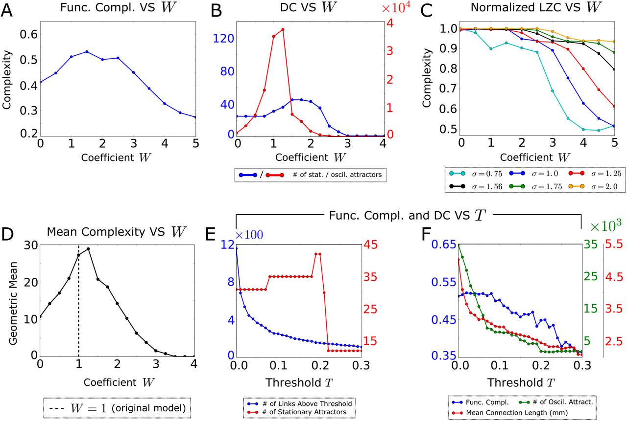
The dependence of these measures of complexity on the inter-hemispheric connectivity scaling parameter W is shown in Figs. 5A-C. All three measures showed a decrease of complexity for high values of W, meaning that abnormally strong inter-hemispheric connectivity would actually reduce activity complexity. An intuitive explanation for this is that excessively strong inter-hemispheric connectivity would increase the overall input current to each cortical area, thereby increasing their firing probability. This results in the formation of a single stationary attractor, where all the areas fire synchronously, and therefore in a strong decrease of the overall complexity of network activity.

A) Functional complexity as function of a global scaling coefficient W that multiplies the inter-hemispheric synaptic weights.
B) Dynamic Complexity (DC), i.e. the number of stationary and oscillatory attractors, as a function of W.
C) Normalized LZC of the spatio-temporal activity pattern. Since the magnitude of the LZC depends on the level of noise, we plotted its dependency for several values of the noise parameter σ (including its best-fit value σ = 1.56), and we normalized the LZC by its maximum over W for each noise level.
D) Geometric mean of the measures of complexity shown in panels A-C, which exhibits a peak for the value corresponding to the real mouse connectome (W∼1).
E) Number of stationary states as a function of the threshold value used for sparsifying the anatomical connectivity, and number of structural connections stronger than a threshold T.
F) Loss of dynamical and functional complexity and mean length of the structural connections, as a function of the threshold T.
Both functional complexity (Fig. 5A) and DC (Fig. 5B) decreased when we used inter-hemispheric connectivity values smaller than the one of real data (W < 1). In this case inter-hemispheric input adds only marginal variability to the total input to each area. As a result, the network accesses fewer attractors and therefore produces a lower DC. Moreover, in the limit W → 0, the two hemispheres become more and more functionally disconnected. In turn, this less rich set of functional connections results in a decreased functional complexity. Functional and dynamical complexity peak for intermediate values of W. The number of oscillatory attractors, which dominates the total number of attractors, has a local peak for the original model of the mouse brain (W = 1), see Fig. 5B.
Unlike the other two measures, LZC (Fig. 5C) did not show a drop at small values of W, but it plateaued over a wide range of W values. Like functional and dynamical complexity, LZC decreased for large values of W. The reason why LZC does not decrease for small values of W is that this measure of complexity reflects variability and diversity of all activity patterns expressed by the network, rather than (as for DC) its ability to generate patterns that can be robustly retrieved through attractor dynamics. When the inter-hemispheric connectivity is very low, activity patterns are highly irregular in both space and time (because the decoupling between hemispheres does not force homologous areas across the hemispheres to synchronize), but the variability of the activity patterns is not sufficient to let the network access a large number of attractors. To summarize these results, in Fig. 5D we plot the geometric mean of the different measures of complexity described so far. The curve shows that the original model (W = 1) features the best trade-off between these measures, therefore suggesting that the mouse brain operates at an optimal working point that maximizes the network variability and versatility.
We next investigated the role of the weakest structural connections in determining the network dynamics. We run the model after thresholding the structural connections with a threshold value T that was systematically varied. The number of structural connections of the mouse cortex with values above T are plotted in Fig. 5E. We studied how the number of stationary (Fig. 5E) and oscillatory (Fig. 5F) model attractors varied with T. The number of stationary attractors was stable until T = 0.2 and then dropped dramatically, suggesting that stationary states are mainly created by a “skeleton” of stronger connections. The number of oscillatory attractors declined steadily and strongly with increasing T, starting from very low T values. This suggests that the weaker anatomical connections create oscillatory attractors, and therefore cover a distinct dynamical role with respect to the stronger connections which regulate the number of stationary attractors (see SI Sec. S4, where we explain analytically this phenomenon). As a result of the decrease in the number of oscillatory attractors, the functional complexity of the network also strongly and steadily decreases with T (Fig. 5F). The weakest links are also the longest, because the mean length of the connections in the network decreases with T (Fig. 5F). Thus, our results support recent suggestions [61] of a possible role of the longest connections in adding variability to network dynamics and FC.
While the functional complexity and the overall DC decrease monotonically with T, LZC was not affected by the removal of structural connections and it has a constant value when T was varied between 0 and 0.3 (not shown). Thus, LZC is less sensitive in detecting the variations of complexity elicited by the variations in the network structural connections.
2.5 Inter-hemispheric non-homotopic attractor dynamics due to inter-hemispheric structural coupling
We next considered the inter-hemispheric topography of the attractor dynamics of the model. Given that excitatory inter-hemispheric coupling should intuitively synchronize homologous areas across the hemispheres, we investigated how the strength of inter-hemispheric structural coupling affects the homotopicity of the attractors. We found (Fig. 6A) that the number of non-homotopic attractors (with mirror-asymmetric activity across the sagittal plane) was small for large values of W, as expected by the simple intuition that strong inter-hemispheric coupling leads to strong inter-hemispheric synchronization. Surprisingly, the number of non-homotopic attractors peaked at intermediate values of inter-hemispheric connection strengths (W∼1) rather than at null inter-hemispheric strength (Fig. 6A). This result was confirmed by computing (Fig. 6B), as function of W, the inter-hemispheric Hamming distance between spiking activity of homologous excitatory populations across the hemispheres, a measure of non-homotopicity that does not rely on computing attractors. The geometric mean of these quantities, which recapitulates the tendency of all these properties, also peaked for W∼1 (Fig. 6C).

A) Number of non-homotopic attractors in the network mode, as a function of the global scaling coefficient W.
B) Mean Hamming distance between the spiking activity patterns of the excitatory populations in the L/R hemispheres.
C) Geometric mean of the non-homotopicity measures showed in panels A and B. Note that the maximum mean non-homotopicity occurs for W = 1, that is the empirical mouse connectome value.
D) Probability distribution of the basins of attraction, calculated numerically from the spiking activity of the model (red bars), and reconstructed by the mapping algorithm when applied to the simulated rsfMRI signals (blue bars), using the attractor structure with homotopicity enforced. Compare this result with Fig. 3F (obtained for mapping the data into the attractor structure of the original model without enforcing homotopicity).
E) Difference between the CAPs of the model with non-homotopic attractors, and the corresponding CAPs as obtained from the model with enforced homotopicity of attractors.
Thus, although our best-fit model exhibited dynamics that was homotopic when averaged over long-time scales of minutes, it does instead predict, for realistic values of inter-hemispheric connectivity (W ∼1), the presence of non-homotopic stationary and oscillatory attractors at the time scale of seconds. This suggests that the dynamics of the mouse rsfMRI may have significant moments of non-homotopic activity originating from its attractor dynamics even if its overall static average is homotopic.
To assess whether the non-homotopicity in the model attractors had a counterpart in the empirical rsfMRI data, we used our algorithm to map the data into either the attractor structure of the original model (as done above in Fig. 3) or to an attractor structure obtained by artificially enforcing homotopicity (see Methods). We found that mapping the empirical data into homotopic model attractors predicted less well attractor occupancy probability than mapping into the original model with non-homotopic attractors (rs = 0.83 vs rs = 0.93, Fig. 6D). This suggests that the non-homotopicity of the attractors space is important to describe the moment-to-moment dynamics of the empirical data.
Furthermore, the importance of non-homotopic moment-to-moment dynamics is also reflected in the reconstruction of the topography of empirical CAPs from the attractors. In Fig. 6E we report the differences between the CAPs of the original model with non-homotopic attractors, and the corresponding CAPs as obtained from the model with enforced homotopic attractor structure. Model CAPs 1 and 6 exhibited significant decrease in the correlation with the corresponding empirical CAPs when using homotopic attractors (see SubSec 4.11). Specifically, the correlation for CAP 1 decreased from 0.59 to 0.56, while for CAP 6 it decreased from 0.56 to 0.51. Thus, the non-homotopicity of attractors explains features of the empirical data that are lost when artificially making them homotopic.
The formation of non-homotopic activity in the presence of inter-hemispheric excitatory coupling is counterintuitive but can be explained within the mechanism, well-established in theoretical physics of interacting systems, of Spontaneous Symmetry Breaking [62]. We report in SI, Sec. S2, an explanation of this mechanism for neural networks.
Together, these results suggest that, while allowing an inter-hemispheric exchange of information through the corpus callosum and the anterior commissure pathways, the cortex can dynamically circumvent structural constraints to process information in parallel between hemispheres.
2.6 Importance of directionality of connectivity and non-linearities in rsfMRI neural dynamics
Our network model included two important aspects of biological plausibility not always present in standard large-scale rsfMRI modelling: directed structural connections and threshold-based non-linear neural dynamics. To test the relative contribution of these features, we compared our whole-brain model to two simpler models obtained either by symmetrizing the structural connections between the excitatory populations (thus making the connectivity un-directed), or by linearizing the network equations. In both cases, we derived a new set of best-fit parameters (Tab. S1), following the same fitting procedure that we used for the original model (SubSec. 4.5).
We first considered how the models reproduced static properties of the empirical rsfMRI data. The Pearson’s correlation between the static across-area distribution of the rsfMRI signals obtained from data and the models (Fig. 7A) was similar across different models, but was higher for our model (p < 10−5, two-sample Welch’s t-test). Moreover, our model was considerably better than the linear one at reproducing the topography of the static FC matrix (Fig. 7A), although it did not outperform the undirected model. However, unlike our model, the undirected and the linear models failed to accurately reproduce the values of the empirical rsfMRI static FC (Fig. 7B). The overlap between the three theoretical FC values distributions and the empirical one was 0.88, 0.55, 0.72 for our model, the undirected and linear models, respectively (Fig. 7B). Thus, directionality of structural connectivity and neural non-linearities help reproducing static aspects of the empirical rsfMRI data.

A) Pearson’s correlation between the cross-area mean rsfMRI activity (left) and the FC matrix (right) of the empirical data, and the corresponding statistics calculated for three network models: “our” model with directed connectivity and non-linear neural dynamics (red), the “undirected” model but with non-linear dynamics but undirected structural connections (green), and the “linear” model with directed structural connections, but with a linear neural activation function (orange). Statistical comparisons were performed by running, for the three network models, 100 groups of 100,000 repetitions each, and then by using a two-sample Welch’s t-test to compare these distributions.
B) Comparison between the probability distributions of the values of the FC matrices. Note that, unlike our model, the undirected and linear models do not fit well the PDF of the experimental datasets. Color coding as in panel A.
C) Number of stationary and oscillatory attractors of the undirected model, as a function of the global scaling coefficient W. Note that the linear model has only one (stationary) attractor.
D) Measures of inter-hemispheric non-homotopicity for the spiking activity patterns of the undirected model.
E) Probability distribution of the basins of attraction, calculated numerically from the undirected model (red bars), and reconstructed by the mapping algorithm when applied to the experimental rsfMRI signals (blue bars). The figure insert shows a zoom of the probability distribution of the stationary attractors in the shaded grey area.
F) CAPs reconstructed from the rsfMRI attractors of the undirected model, and their Pearson’s correlation with the corresponding empirical CAPs of Fig. 3H.
We next considered how different models accounted for the empirical rsfMRI moment-to-moment dynamics. We found a major reduction in the number of attractors, and thus of the dynamical complexity, generated by the undirected and the linear model compared to our model (Fig. 7C). The undirected model generated much fewer attractors than the original model. For W = 1, we found only 6 stationary states in the undirected model, compared to 31 stationary states in our model (Tabs. S2 and S3), and 8,958 rather than 34,877 oscillations. Moreover, while our model exhibited the largest number of attractors at W∼1 (Fig. 5B), the dynamical complexity and attractor numbers of the undirected model peaked at W = 0.5 (Fig. 7C). Thus, the undirected model exhibits poorer attractor dynamics, which would not be maximized by values of inter-hemispheric anatomical connection strength equal to those of the mouse brain. Similarly, indices of non-homotopic activity (i.e. diverging activity across some of the homologous areas in the two hemispheres) similar to those considered in Figs. 6A, B did not peak (Fig. 7D) at W∼1 for the undirected model, as it happened for our model (Fig. 6).
Importantly, we found that the empirical rsfMRI time series did not map well into the attractors of the undirected model. The Spearman correlation between the probability of occupancy of the attractors predicted by the model and the distribution reconstructed by the mapping algorithm was not significant (rs = 0.43, p = 0.34, Fig. 7E), and the undirected model was particularly bad at describing the relative probability of stationary attractors (insert of Fig. 7E). The impoverishment of attractor dynamics in the undirected model led also to a much poorer reconstruction of the topography of the empirical CAPs from its attractor basins (cf. Fig. 3I with Fig. 7F). Thus, the undirected model lacks the ability to predict, from attractor dynamics, the features of most experimentally observed CAPs.
The attractor dynamics of the linear model was even poorer, as it exhibited only one stationary attractor (which is always stable for W ∈ [0, 16.4]). Given that there was only one attractor, we did not attempt to map CAPs and attractors in this model.
In sum, the neural non-linearities and the directionality of the anatomical connectivity inserted in our model only marginally increased the accuracy of model predictions of the static properties of empirical rsfMRI data. However, the non-linearities and the directionality information of the connectome deeply affected the fast network dynamics on the scale of seconds. Specifically, they were crucial to create richer attractor dynamics in the model, which ultimately allowed the model to better explain moment-to-moment CAPs of empirical data.
2.7 Model-based estimation of excitation-inhibition balance in cortical resting-state dynamics
Given that our model included excitatory (E) and inhibitory (I) populations in each area, we finally examined which local E-I interaction patterns emerged from the best-fit model. We first investigated the balance between E and I currents received by either E or I populations in each area. The model predicts that during resting state activity this balance is such that the total input current to each population (the signed sum of the E and I input currents) fluctuates relatively close to the threshold for firing (Fig. 8A). Consequently, the time-averaged spiking activity in both the E and I populations in each area (Fig. 8B) was at an intermediate level of 0.4 to 0.7, measured in a normalized scale in which zero indicates total silence and 1 indicates continuous firing always saturated at the maximal level. The overall E-I balance is further highlighted by the finding of a linear relationship between the total input current to the I population and the total input current to the E population in each cortical area (Fig. 8C), meaning that the areas with higher total input current to the I population have also a proportionally higher input current to the E population, which maintains E-I interactions balanced.

A) Fluctuations of the total (i.e. E plus I) input currents to each cortical population. Excitation and inhibition balance each other, meaning that the E-I currents sum up to produce total currents fluctuating around the firing threshold (dashed horizontal line).
B) Mean spiking activity of the cortical populations.
C) Linear relationship between the total currents to the E-I populations.
D) Ratio of the E-I components of the currents to each cortical population. The ratio is nearly constant for the inhibitory populations (red curve), while the excitatory populations of the DMN show a much larger ratio than the other excitatory subnetworks (blue curve).
E) Sensitivity of our model to external stimulation is maximum at rest, thereby suggesting a functional benefit of the balanced state. To evaluate sensitivity, we first computed the response to the perturbation, averaged over the 10 simulation time steps following the stimulus, as a function of the perturbation strength, and then we quantified sensitivity as the derivative of the response with respect to the strength of the applied input current.
F) E-I linear relationship and its functional benefit, as a function of a global scaling factor z, which multiplies the synaptic weights between the E-I populations. Note that the sensitivity to stimulation is almost maximum for our model (i.e. for z = 1), and that the linear relationship between the total currents vanishes for large z.
While there was a proportionality of the total currents received by E and I populations in the same area, some areas had a higher ratio of E/I input currents. In particular, areas in the DMN, which had high activity both in empirical and model rsfMRI time series, and whose total currents to E neurons fluctuated slightly above the threshold in the model (Fig. 8A), received a higher proportion of E input currents to the E population (Fig. 8D). The ratio of E/I input currents received by the I populations remained relatively stable across areas (Fig. 8D). Note that during the fitting procedure we did not attempt to achieve neither the linear relationship between the total input currents to the E-I populations, nor the balance of the mean firing rates described above. These properties emerged in the dynamics of our best-fit network.
We next investigated the functional consequence of the locally balanced nature of the E-I interactions predicted by our model. We computed the sensitivity of the response of the whole cortex to the application of an external perturbation current to all the populations. Results (Fig. 8E) indicate that the sensitivity is maximal around the value of 0 (unperturbed resting state activity) for the input current. This is because in the resting configuration the total input currents on each cortical area fluctuate around the firing threshold (see Fig. 8A), where weak perturbations in the stimulus intensity elicit the largest variations in activity. In sum these results suggest the presence of a balanced nature of E-I local interactions in resting state activity, and a possible advantage of high sensitivity to perturbation (and thus high stimulus information coding capabilities) of the resting state configuration.
To highlight the importance of the E-I interactions predicted by the parameters of the best-fit model, we multiplied the synaptic weights of the local E to I and I to E structural connections by a global scaling coefficient z, so that the E-I populations are structurally disconnected when z = 0, while they are connected by the best-fit weights when z = 1. We then studied the network dynamics as a function of the rescaling parameter z. We found that both the linear relationship between total input currents to E and I populations and the sensitivity of cortical activity to the application of an external input current peaked at the z ∼ 1 value, corresponding to the parameter values estimated by the model best fit to the empirical rsfMRI data. This suggests that the mouse brain at rest not only keeps E and I interactions balanced, but also that this balance is optimal for encoding of external stimuli.
3 Discussion
Recent years are witnessing a growing interest in modelling and understanding the dynamics of rsfMRI activity, not only in the human brain but also across species. This work has prominently included measuring and modelling the rsfMRI of the mouse brain [35-38]. The mouse has the unique advantage of the availability of a precise measure of the whole-brain axonal connectivity and its directionality [21-23,42]. Here we contributed to this endeavor by developing a novel whole-brain model of the resting state activity of the mouse cortex.
Our work adds novel concepts and predictions to both existing mouse whole-brain modelling and other similar models developed for humans [6,8-10,13]. Specifically, our model made new predictions about the dynamics of resting mouse cortex in terms of attractor dynamics over fast time scales of seconds, which we successfully validated against several key findings in the empirical data. We also manipulated the model’s structural connectivity to make novel predictions about how its structure generates complexity of dynamics and inter-hemispheric non-homotopic activity.
3.1 Progress with respect to previous rsfMRI models in studying whole-brain attractor dynamics
Most whole-brain models simulate the rsfMRI signals either by modeling neurovascular coupling with a synaptic gating variable [9-11,13,63], or by employing neural mass models [6,12,14,15,64]. Our model instead uses a binary non-linearity for describing neural spiking activity. Such binary firing rate models have been rarely used for whole-brain networks [5,7], but are of great interest because they generate attractor dynamics in finite configurations space, which can be studied by combining analytical methods with state-of-the-art numerical techniques [43]. Attractor dynamics is a major theoretical feature of recurrently connected neural networks, yet its presence in large-scale brain dynamics has been only seldomly investigated (see e.g. Refs. [7,13] modelling the human brain). Our work adds to and expands previous attempts to predict attractor dynamics from large scale models in several ways.
First, the numerical formalism we used allows an exhaustive coverage of attractor states including stationary and periodic attractors. For example, in our model with a parcellation into 34 areas we could map 31 stationary attractors and thousands of oscillatory attractors, whereas previous work mapped no oscillatory attractors in humans [7,13] and investigated simple oscillatory dynamics in a mouse model with binary structural connections [38]. The ability to map extensively attractors was an advance of technical nature, but it was essential to characterize the properties of moment-to-moment, fast scale dynamics of the model and to compare it with the dynamics of empirical rsfMRI data on a time scale of seconds. This allowed us to provide predictions and mechanistic hypotheses about possible novel dynamic features such as inter-hemispheric non-homotopicity and aspects of dynamic complexity imputable to attractor dynamics. These predictions go beyond previous seminal work on attractor dynamics in humans, which was primarily focused in relating attractor dynamics to time-varying FC [7,13].
Second, our study extended previous work on attractors in the human brain to the mouse brain. This allowed us to investigate the role of the directionality of anatomical fibers, a feature not available to a comparable extent for the human brain, in shaping attractor dynamics. We found that the richness of attractor dynamics and the good match between empirically rsfMRI dynamics and attractor properties was found only when considering the directionality of the anatomical connectivity of the real mouse brain. Using an undirected version of the anatomical connectivity matrix (conceptually similar to that measured with DTI) led to an impoverishment of the model’s attractor landscape and of the ability to predict real rsfMRI dynamics.
Third, our study of empirical mouse rsfMRI time series with an attractor mapping algorithm found a topography of putative attractors and a dynamics of attractor basin occupancy compatible with that predicted by the model. These results suggest that attractors dynamics explains some features of resting state activity. The evaluation of plausibility of attractor dynamics on empirical rsfMRI data was facilitated by the fact that in our model the structure of the basins of attraction and the probability with which each basin is visited over time during spontaneous dynamics was the same both for spiking activity and for the rsfMRI activity, or, in other words, attractor dynamics in the model was invariant to transformations of neural activity into rsfMRI. This property held also for the relative distribution of activity over areas, but did not hold for the static FC metric [65], which was similar in shape but had different distribution of values when comparing spiking and rsfMRI activity in the model.
Finally, we were able to relate quantitatively attractor dynamics to CAP dynamics found on the scale of seconds in empirical data. The possible origin of these CAPs in terms of neural processes has been debated. CAPs may reflect a variety of neural phenomena, including inter-areal connectivity, widespread cortical changes associated with changes in brain state, and brief, event-like activity rather than sustained and possibly oscillatory interactions [33]. However, there is still relatively little understanding in terms of models of how CAPs may originate. Importantly, our model also provides a possible mechanistic explanation that relates the emergence of CAPs to anatomical cortico-cortical connectivity. Since attractor dynamics originates from the underlying anatomical inter-areal connections, our work provides model-based evidence that CAPs reflect at least in part the result of neural interactions across areas, and it explains how they may mechanistically arise from generating attractors. Because attractors represent minima in the energy landscape of the network, our work also suggests that changes in CAPs can be taken as indicators of changes in the energy landscape of the brain, a topic of current active research [40]. Future studies will determine how the interaction between such attractor cortical dynamics and neuromodulatory systems such as the ascending arousal system may shape the energy landscape of the cortex [40]. The ability of the model’s attractors to explain empirical CAPs emerged even though the model was fitted only to maximize static features of rsfMRI activity, not its seconds-scale dynamics. Thus, the insurgence of network states reminiscent of empirical co-activation patterns represent a genuine prediction of the model.
By enabling to relate anatomical connectivity, attractors and rsfMRI CAPs our formalism might be crucially employed in future studies to make empirically testable predictions about how alterations of the connectome resulting from injury or neurodegenerative disorders may alter seconds-scale brain dynamics.
3.2 Model predictions of rsfMRI functional connectivity properties
It has been long established that network models with realistic anatomical connectivity can fit well the static long-time rsfMRI FC. Our model confirms this finding. In this respect, it was notable that our model predicted the presence of relatively strong inter-hemispheric FC between homologous areas across hemispheres. This strong FC is present in empirical data, but has not been robustly attained in previous models [9,10,36].
Importantly, our model predicted well the empirical FC obtained after regressing out the global signal, even if its parameters were not fitted to predict it, thereby reinforcing the power of our model to capture real-data dynamic features beyond what it was optimized to reproduce. While static FC had all positive entries, the regressed FC showed interesting patterns of anti-correlations across areas that were also visible in CAPs and were predicted well by the model. These results contribute to the ongoing debate about the validity and significance of global signal regression in rsfMRI [66]. While some studies consider the global signal as source of noise, promoting global signal regression as a crucial preprocessing step for removing residual head motion [67], other studies provided robust evidence for considering the global signal a real neural phenomenon, highlighting how it relates to FC topography [68-70], and to CAPs topography and dynamics [28,29]. The observation that our model predicts features of regressed signals only from modelling how interactions between cortical areas shape whole cortex dynamics, supports the notion that the global rsfMRI signal potentially carries important information about how different areas interact to produce brain dynamics.
3.3 Model predictions on the relationship between anatomical connectivity and seconds-scale whole-brain dynamics
Our work explored the role of inter-hemispheric anatomical connectivity by rescaling in the model its strength with respect to the original structural connectivity matrix, and by studying how inter-hemispheric connectivity strength variations affect the seconds-scale rsfMRI dynamics. By doing so we obtained notable predictions. First, values of inter-hemispheric connectivity similar to those found in the real mouse brain maximize the number of attractors, and thus dynamic complexity of the moment-to-moment activity. Larger or smaller values of inter-hemispheric connectivity would generate much smaller values of attractors numbers and dynamic complexity. We speculate that dynamic complexity may have an impact on the function of the brain because it represents the repertoire of brain states that can be reliably and dynamically generated starting from arbitrary initial conditions. Therefore, larger values of this complexity may enable a larger repertoire of information processing capabilities. Fitting our model to rsfMRI activity under different behavioral states could help validating empirically a possible role in brain function of the dynamic complexity we evaluated here.
Second, values of inter-hemispheric connectivity similar to those of the real mouse brain not only led to higher dynamic complexity, but also to higher values of inter-hemispheric non-homotopicity in seconds-scale cortical activity. Despite our model included an inter-hemispheric homotopic axonal connectivity matrix, it predicted the formation of significant differences between the dynamics of the two hemispheres. This inter-hemispheric non-homotopicity was predicted by the model to happen only over fast timescales (of the order of seconds), and was averaged away when static activity and FC were computed over the several minutes of a whole rsfMRI time series. Our model predicts that this phenomenon arises from spontaneous symmetry breaking originating as a consequence of the strong difference between the strength of the intra and inter-hemispheric structural connections. This functional symmetry breaking may provide the brain with the possibility to exhibit some degree of parallelization between information processing across hemispheres. With this mechanism, the mouse brain might efficiently partition the computational load between its hemispheres, so that one can work independently from the other, while allowing at the same time inter-hemispheric information transfer. These model predictions suggest that the observed levels of inter-hemispheric connectivity may provide a good trade-off between dynamic complexity and parallel information processing. The predictions could be further tested in future investigations by fitting our model to rsfMRI activity in animals with impaired inter-hemispheric connectivity, to evaluate how the number of attractors and the structure of attractor dynamics may vary under these conditions.
Finally, by studying the model’s dynamics after thresholding the weakest connections, we predicted that the number of stationary attractors is more sensitive to the strongest anatomical connections (which on average select shorter connections, see Figs. 5F and S1B), while the number of oscillatory attractors, which exceed the stationary ones by at least three orders of magnitude, is highly sensitive to the presence of the weaker connections (which are also on average the longer-distance ones). These model predictions suggest a possible role of long-distance pathways in shaping dynamics, compatible with model predictions obtained recently based on very different analysis formalisms [61]. Under the assumption that larger attractor numbers and higher dynamical complexity help information processing, these results are also compatible with other recent model-based proposals that long-range connections enhance information processing in the brain [15].
4 Materials and methods
4.1 Resting state fMRI data acquisition
The rsfMRI dataset used in this work consists of N = 15 scans in adult male C57Bl6/J mice. These datasets were published previously[28]. The full rsfMRI time series were made publicly available in these previous publications. As described in the original publications, all in vivo experiments were conducted in accordance with the Italian law (DL 26/214, EU 63/2010, Ministero della Sanità, Roma) and the recommendations in the Guide for the Care and Use of Laboratory Animals of the NIH. Animal research protocols were reviewed and consented by the animal care committee of the Italian Institute of Technology, and Italian Ministry of Health.
Animal preparation, image data acquisition, and image data preprocessing for rsfMRI data have been described in full detail elsewhere [28,30,31]. Briefly, rsMRI data were acquired with a 7.0 Tesla scanner (Bruker Biospin, Ettlingen) using a 72 mm birdcage transmit coil, and a four-channel solenoid coil for signal reception. Single-shot EPI time series were acquired using the following parameters: TR/TE 1200/15 ms, flip angle 30°, matrix 100 × 100, field of view 2 × 2 cm2, 18 coronal slices, slice thickness 0.50 mm, 500 (n = 15) volumes and a total rsfMRI acquisition time of 10 minutes, respectively. As in [28], rsfMRI time series preprocessing included: removal of the first 50 frames (1 minute), despiking, motion correction, and spatial normalization to an in-house mouse brain template with the same native resolution as raw EPI volumes. Head motion traces and the mean ventricular signal (average rsfMRI time series within a manually-drawn ventricle mask from the template) were regressed out. The resulting images were band-pass filtered using a 0.01 – 0.1 Hz band, spatially smoothed using a Gaussian kernel of 0.5 mm FWHM, and z-scored voxel-wise.
4.2 Parcellation
We employed the coarsest parcellation (i.e. highest hierarchical level) available in the Allen Mouse Brain Atlas to extract resting-state time series from 34 cortical regions (17 for each hemisphere) as described in [21].
4.3 CAPs
To identify CAPs in empirical rsfMRI data we used the mean CAP map templates derived in [28]. Briefly, these CAPs were identified by clustering the concatenated rsfMRI frames of N = 15 subjects using the k-means++ algorithm [71], with 15 replicates, 500 iterations, and Pearson’s correlation as distance metric. Previous work [28,29] defined k = 6 as an optimal number of clusters satisfying criteria of algorithm stability, high variance-explained, and reproducibility between independent datasets. The clustered rsfMRI frames were voxel-wise averaged into CAP maps, and these were then parcellated using the above-mentioned regions by averaging the rsfMRI activity of the voxels within the region of interest in each CAP map.
4.4 Neural network model
Our network model of the mouse cortex is composed of 34 areas (17 for each hemisphere), labelled in Fig. 1A. In turn, each of these areas is composed of one excitatory (E) and one inhibitory (I) population. The excitatory populations are recurrently connected by the 34 × 34 directed structural connectivity matrix JE,E. Each entry of JE,E was estimated from the mouse connectome [22] as the number of connections from the entire cortical source region to the unit volume of the cortical target region [47], multiplied by a global scaling coefficient GE,E, which represents the average synaptic efficacy per unit of structural connectivity strength and is assumed to be constant across all pairs of areas. Note that, in keeping with previous investigations [21], the matrix JE,E is structured such that the R to R and R to L connections originating from the R hemisphere are respectively identical to the L to L and L to R connections originating from the L hemisphere.
Each excitatory population was connected locally to its corresponding inhibitory population. The weights of the I to E, E to I and I to I connections were collected in the matrices JE,I, JI,E and JI,I. The values of the entries of these matrices were determined by best fit. The matrices JI,E and JI,I were constructed to have the same value across all areas, whereas the matrix JE,I had values that could be different across areas. This was because in preliminary runs of the model we verified that having area-dependent JE,I seemed to improve the fit quality, whereas having entries of JI,E and JI,I that were area-dependent seemed not to improve fit quality (see also [9]). Since the values of JE,I, JI,E and JI,I were determined by best fit rather than by anatomical measures, it was not necessary to include a scaling coefficient representing synaptic efficacy, because this scaling was effectively determined by the best fit.
The mean firing rate of the i-th population in the time interval [t, t + 1) is described by the binary variable Ai(t), so that Ai(t) = 0 if the population is silent at time t, while Ai(t) = 1 if it is firing. The spiking activity vector collecting the firing rates of the 68 cortical populations, can switch over time among a set of 268 ≈ 3 × 10²⁰ distinct activity patterns. The spiking activity evolves at discrete time instants, where the time step corresponds to the repetition time TR = 1.2s. It should be noted that the variations of the model’s spiking activities that are updated from frame to frame should not be interpreted as variations of firing within an integration time constant of the neurons, but rather as time-averaged variations in neural activity on the time scales of the rsfMRI frame rates.
In each population, the incoming synaptic weights are multiplied by the presynaptic activities at time t, to produce the total postsynaptic current. Then, by adding this current to a noise term expressing the net effect of stochastic components of neural activity, we get the mean membrane potential of that population (see Fig. 1B). The membrane potential is passed through a threshold-based activation function, whose output Ai(t + 1) represents the mean activity of that population at the next time instant. If the membrane potential is below a firing threshold Vthr, then Ai(t + 1) = 0, otherwise Ai(t + 1) = 1. Note that the cortical populations do not receive any afferent currents from subcortical regions.
The noise sources in the model are independent and normally distributed, with standard deviation σ, as typically used in whole-brain models (e.g. [5,10]). These noise sources include all sources that could make neural activity stochastic [72].
To summarize the above with a compact set of equations, we sorted the 68 network nodes so that the excitatory (E) populations are labelled by the indexes i ∈ {1, ⋯, 34}, while the inhibitory (I) populations by the indexes i ∈ {35, ⋯, 68}. The mean firing rate of the i-th population at time instant t, namely Ai(t) ∈ {0, 1}, is updated at discrete time instants as follows:
 for i ∈ {1, ⋯, 68}. The matrix Ji,j has entries from JE,E, JE,I, JI,E or JI,I depending on the index value. In Eq. (1), Vi is the mean membrane potential of the i-th population, and Vthr is the threshold for firing. 𝒜(⋅) represents the activation function of the network. For our model and for the undirected model discussed in SubSec. 2.6, 𝒜(⋅) is the Heaviside step function:
 In the linear model reported in the SubSec. 2.6, 𝒜(x) = x. Moreover,
  is a set of normally distributed sources of neuronal noise, with mean zero and standard deviation σ. The noise terms are spatially and temporally independent, namely Corr (𝒩i(t), 𝒩j(s)) = 0 ∀i, j, t, s when i ≠ j and/or t ≠ s. In Eq. (1), ℑsub represents the total afferent current originating from subcortical regions. Since we assume that subcortical currents (in particular sensory stimuli from the thalamus) are negligible at rest, in this paper we set ℑsub = 0, with the only exception being the study in SubSec. S4 of the stability of the network attractors as a function of ℑsub.
We modeled the rsfMRI activity in each cortical area as the total postsynaptic currents on the corresponding excitatory populations. This model seemed in our attempts to provide better fits to the data (especially on the FC values, see SubSec. 2.1) than using the spiking activity.
The model has a set of free parameters, namely GE,E, JE,I, JI,E, JI,I, Vthr, σ. Their values, which are reported in Tab. S1 of the Supplementary File, have been obtained by fitting the model to the static values of mean activity and FC of real mouse rsfMRI data, as detailed in SubSec. 4.5.
4.5 Fitting procedure
In this section we describe how we calculated the values of the free network parameters introduced in SubSec. 4.4, namely the global scaling coefficient of the structural connectivity (GE,E), the strengths of the I to E, E to I, I to I connections (JE,I, JI,E, JI,I, respectively), the membrane potential firing threshold (Vthr), and the standard deviation of the noise sources (σ). We derived the best estimates of these parameters through a random grid search, by finding the values that could describe reasonably well the time-averaged first- and most second-order statistics of the mouse rsfMRI activity. Specifically, the first-order statistic that we considered in the fitting procedure is the relative across-area distribution of the time-averaged rsfMRI activity (see SubSec. 4.5.1), while the second-order statistics are several properties of the across-subject averaged functional connectivity matrix (see SubSec. 4.5.2). We calculated the first- and second-order statistics over the whole time series, which comprise 450 time points each. Moreover, the experimental statistics have been averaged over 15 mice, while the theoretical statistics over 100 repetitions of the network.
Then, we used the best-fit parameters to test if the model could predict and explain not only the rest of second-order statistics that were not used to set the parameters (specifically, the functional connectivity matrix obtained after global signal regression, see Fig. 4), but importantly also finer time-dependent features of the dynamical organization of the mouse rsfMRI activity (namely the probability with which the basins of attraction are visited over time, and the spatial similarity between them and CAPs, see Fig. 3).
In what follows, we describe in detail the statistics that we used for linking the model to the experimental datasets. The values of the best-fit parameters so obtained are listed in Tab. S1.
4.5.1 Relative across-area distribution of the time-averaged rsfMRI
The time-averaged mean of the rsfMRI signals is a first-order statistic that has been typically employed in functional neuroimaging studies to measure the central tendency of the activity [73]. Here, we calculated the relative across-area distribution of the time-averaged rsfMRI across the 34 cortical areas of the mouse cortex, and normalized it by subtracting the value of the global signal (that is, the average over all cortical areas of the rsfMRI signal [9]) from the mean signals of each area and finally dividing the resulting values by the maximum absolute value across all areas, obtaining a normalized vector whose entries lie in the range [-1, 1].
During the fitting procedure, we maximized the spatial similarity between the distributions obtained from the empirical and model rsfMRI signals, see Figs. 2A and 2B. This similarity is measured by the Pearson’s correlation coefficient across their 34 entries, which is calculated as reported in SubSec. 4.6.
4.5.2 Static Functional Connectivity matrix
The static Functional Connectivity (FC) matrix was computed as the cross-area Pearson’s correlation estimated over the whole time series and calculated without global signal regression (see Figs. 2D and 2E). To select the best-fit values that maximize the similarity between the rsfMRI FC matrices of the empirical mouse data and of the model, we minimized the mean absolute difference between the two FC matrices. We verified that the fine-tuned best-fit parameters maximized also the overlap [74] of the probability distributions of the entries of the FC matrices. As a consequence, this also minimized the difference between the mean values of the FC matrices. These parameters also maximized the Pearson’s correlation and the Lin’s concordance correlation coefficient (CCC) [75] between the empirical and model FC matrices. Note that, while the Pearson’s correlation captures similarity in the shapes of the FC matrices regardless of the actual values, the Lin’s coefficient captures also the similarity of the values and thus is high when the two matrices are similar both in shape and distribution of values. Often model parameters in whole brain modelling are chosen to maximize only the similarity between model and data of the Pearson’s correlation of the FC matrices, but giving an overall distribution of actual values which may differ substantially between model and data. Here we succeed in explaining well both the shape of the FC matrix and the distribution of its values.
We also verified that the best-fit parameters maximized the Lin’s CCC between the model and data FC matrices computed when focusing only on the regions in the L/R hemispheres with the highest average resting state mean activity, (VIS, RSP, PTLp, ACA, PL, ORB, ILA, AI, MO, SS).
Finally, following [9,10], we also calculated the dominant spatial mode or first principal component of the rsfMRI signals, namely the first eigenvector of their covariance matrix. Then we verified that our best-fit parameters also maximized the similarity between the normalized dominant modes of the empirical and model signals, which was quantified by their vector projection or dot product.
Overall, the set of chosen best-fit parameters accounted well for many properties of the static FC of the empirical rsfMRI data.
4.6 Calculation of the correlation coefficients
We calculated numerically the Pearson’s correlation and its p-value through the function stats.pearsonr() of the Python library Scipy [76] (source code available for download at https://www.scipy.org/), and we computed its 95% confidence interval from the Fisher’s transformation. We calculated the Lin’s correlation from the Pearson’s correlation, the mean and the standard deviation of the matrix entries, as reported in [75].
As is common practice (see e.g. [9,36]), when evaluating the similarity between the model and empirical FC matrices, we calculated the Pearson’s and Lin’s correlation coefficients between the full (i.e. 34×34) matrices, or between symmetric partitions of those matrices (e.g. Figs. 4D and 4E), by arranging the entries above their main diagonals as vectors, and then by applying the measures of correlation/concordance to the resulting vectors. For asymmetric partitions (e.g. Figs. 4F and 4G), we used the whole set of entries to construct the vectors.
In SubSecs. 2.2 and S3, we evaluated numerically the similarity between the occupancy probabilities of the basins of attraction by their Spearman’s correlation, through the function stats.spearmanr() of Scipy [76]. The reason for preferring the Spearman’s correlation over other measures of similarity in our analysis of SubSecs. 2.2 and S3, is that it is less sensitive to outliers, and therefore it allows us to better discriminate the differences in the similarity between the probability distributions, when varying the coefficient W (see Figs. 3C, F and S3A-C). Note indeed that the probability distributions in Figs. 3C, F all had one outlier, namely the probability to observe the network state in any oscillatory basin, which is considerably larger than the occupancy probabilities of each of the 31 stationary attractors.
4.7 Community detection
The community structure of the functional network shown in Fig. 2I was derived using the leading eigenvector method [52], implemented in the function community_leading_eigenvector() of the Python library igraph [77]. Source code available for download at https://igraph.org/python/.
4.8 Attractors detection
We detected the spiking activity attractors by initializing the network model with a random activity pattern. Then we allowed the pattern to evolve stochastically under the effect of noise for a given number n of time steps (typically n = 100, so that the network statistics become stationary). At every time step, the spiking activity pattern was updated by solving iteratively Eq. (1) of Methods. After n time steps we turned off the noise sources, so that the spiking activity could converge to an attractor of the network without jumping randomly between several attractors. This procedure was then repeated 100,000 times starting from distinct initial patterns, in order to detect the largest number of attractors.
Note that the above algorithm is not guaranteed to find the whole set of attractors, especially when the number of network repetitions is small compared to the total number of attractors. While this algorithm can fully detect the relatively small set of stationary attractors in a few thousands of network repetitions, typically it can reconstruct the prohibitively large set of oscillatory attractors only partially.
To cross-validate our results, we calculated the number of stationary states in a second, alternative way, which relies on the optimized brute-force algorithm introduced in [43]. We used an improved version of that algorithm (described in SubSec. S1), which allowed us to find the stationary attractors of the network in the set of 268 ≈ 3 × 10²⁰ activity patterns. Unlike the algorithm described at the beginning of this section, this other algorithm is guaranteed to reconstruct the whole set of stationary states, but in [43] it was optimized specifically for networks with sparse structural connections. For this reason, the brute-force algorithm proved useful in the validation of the red curve in Fig. 5E (which shows the variation in the number of stationary attractors as a function of the network sparseness, see SubSec. 2.4 for more details) for T ≥ 0.05. Reassuringly, the two algorithms provided the same number of stationary attractors.
4.9 Attractor mapping algorithm
In Fig. S2C we sketch the logic of our mapping algorithm. Its main ingredient is a classifier, which labels each time frame of the to-be-analyzed (empirical or model) rsfMRI time series with the index of the attractor that is more likely to having generated it. The algorithm takes the z-score of the to-be-analyzed 34-dimensional rsfMRI signal (which is calculated in the preprocessing block of Fig. S2C at every time instant), and compares it (by computing Euclidean distance) with the z-score of the 34-dimensional model rsfMRI activity, averaged over the basins of each attractor. This provides a measure of distance between rsfMRI activity at each time point and each attractor. At every time instant, the classifier labels each time point of the to-be-analyzed rsfMRI times series with the index of the attractor exhibiting the shortest Euclidean distance (see Fig. S2D). By counting the number of data points across the time series that are assigned to each attractor, we infer the probability of occupation of the basin of each attractor (blue bars in Figs. 3C, F). To provide a measure of the topography of each estimated basin of attraction that can be compared with the topography of the basins of the network model, the mapping algorithm calculates the mean of the z-score of the to-be-analyzed rsfMRI signal on all the time points that the classifier assigned to each attractor. Example comparisons are shown in Figs. 3A, D for attractor #17, and in Figs. 3B, E for attractor #13.
4.10 Calculation of Lempel-Ziv complexity
We calculated the Lempel-Ziv complexity (LZC) of the matrix of the model’s spiking activity of all areas concatenated over all simulated time points by applying the algorithm introduced in [78]. To make the complexity measure minimally dependent on the total amount of activity and maximally dependent on the formation of spatial patterns in the data, LZC was normalized by LH(L)/log_2(L), where L is the total number of spatio-temporal spiking activity samples, while H(L) is the entropy of the 34 cortical regions. The normalized LZC increases with the number of distinct spatial patterns of spiking activity occurring at a given time instant, and not occuring at previous instants [79].
4.11 Methods to assess non-homotopicity in attractor structures
To assess whether the non-homotopicity in the model attractors had a counterpart in the empirical rsfMRI data, we mapped the empirical rsfMRI data either by respecting the differences between non-homotopic attractors (that is, as in Fig. 3F we mapped each rsfMRI data point into the basins of each of the 32 attractors) or by artificially eliminating the differences between the non-homotopic attractor pairs (this was made by pooling the two basins of attraction of two mirror-symmetric attractors (e.g. attractors #2,6) into only one basin prior to the attractor mapping). To compute the effect of enforcing homotopicity on the reconstruction of the CAP topography from the model’s attractors, we run the mapping algorithm 100 times, for both the original model with non-homotopic attractors and the model with enforced homotopic attractor structure, and in each run we evaluated against real data the accuracy of the CAP reconstructed topography through 100,000 repetitions of the network models. In each of the 100 runs we calculated the Pearson’s correlation between the empirical CAPs and the reconstructed CAPs. We performed a Welch’s t-test to assess whether the sets of correlations generated by the two models had equal means. Moreover, we checked that these two significantly different sets of correlations have non-overlapping ranges of one standard deviation from their means.
Acknowledgements
We acknowledge the support from the NIH Brain Initiative (U19 NS107464, R01 NS109961, R01 NS108410 to SP and 1R21MH116473-01A1 to AG), the European Research Council (ERC) under the European Union’s Horizon 2020 research and innovation program (#DISCONN; no. 802371 to AG), Brain and Behavior Foundation (NARSAD Independent Investigator Grant #25861 to AG), and the Telethon foundation (GGP19177 to AG). The funders had no role in study design, data collection and analysis, decision to publish, interpretation of results, or preparation of the manuscript.
References
- [1].↵
- [2].
- [3].↵
- [4].↵
- [5].↵
- [6].↵
- [7].↵
- [8].↵
- [9].↵
- [10].↵
- [11].↵
- [12].↵
- [13].↵
- [14].↵
- [15].↵
- [16].
- [17].↵
- [18].↵
- [19].
- [20].↵
- [21].↵
- [22].↵
- [23].↵
- [24].↵
- [25].↵
- [26].
- [27].↵
- [28].↵
- [29].↵
- [30].↵
- [31].↵
- [32].
- [33].↵
- [34].↵
- [35].↵
- [36].↵
- [37].
- [38].↵
- [39].↵
- [40].↵
- [41].↵
- [42].↵
- [43].↵
- [44].↵
- [45].↵
- [46].↵
- [47].↵
- [48].↵
- [49].↵
- [50].↵
- [51].↵
- [52].↵
- [53].↵
- [54].↵
- [55].↵
- [56].
- [57].
- [58].↵
- [59].↵
- [60].↵
- [61].↵
- [62].↵
- [63].↵
- [64].↵
- [65].↵
- [66].↵
- [67].↵
- [68].↵
- [69].
- [70].↵
- [71].↵
- [72].↵
- [73].↵
- [74].↵
- [75].↵
- [76].↵
- [77].↵
- [78].↵
- [79].↵


