

Abstract
Bounded temporal accumulation of evidence is a canonical computation for perceptual decision making (PDM). Previously derived optimal strategies for PDM, however, ignore the fact that focusing on the task of accumulating evidence in time requires cognitive control, which is costly. Here, we derive a theoretical framework for studying how to optimally trade-off performance and control costs in PDM. We describe agents seeking to maximize reward rate in a two-alternative forced choice task, but endowed with default, stimulus-independent response policies which lead to errors and which also bias how speed and accuracy are traded off by the agent. Limitations in the agent’s ability to control these default tendencies lead to optimal policies that rely on ‘soft’ probabilistic decision bounds with characteristic observable behavioral consequences. We show that the axis of control provides an organizing principle for how different task manipulations shape the phenomenology of PDM, including the nature and consequence of decision lapses and sequential dependencies. Our findings provide a path to the study of normative decision strategies in real biological agents.
Making the right decision often depends on specifying accurately the state of the environment. In these conditions, it is often useful to wait and gather more evidence before committing to a course of action. Indeed, organisms are able to accumulate evidence across time in order to make better decisions in the presence of sensory uncertainty1–3. Decades of experimental and theoretical work have shown that this process is accurately captured by the framework of bounded evidence accumulation4,5. In this framework, the outcome and timing of a categorical decision are specified as the moment in which a decision variable – keeping a running count of the relative evidence favoring each alternative – attains a given magnitude (referred to as the decision bound) for the first time.
While many variants of this general scheme have been developed and are used due to their ability to accurately describe choice and reaction time (RT) data from psychophysical experiments3,4,6–10, these models are, in addition, attractive due to their normative grounding: they describe not only how agents decide, but how they ought to decide in order to satisfy reasonable decision goals. Wald’s 1945 sequential probability ratio test11 (SPRT) provides an optimal prescription12 for choosing online between two known alternatives, or hypothesis, during the sequential observation of the samples they produce. The SPRT requires temporal accumulation of a form of sensory evidence until a certain bound – which specifies the probability of choosing incorrectly – is reached, and is optimal in the sense of requiring, on average, the least number of observations for a given error rate. The SPRT formalizes a speed-accuracy tradeoff (SAT), as accumulating enough evidence to make good decisions takes time. This is the essential computational problem in sequential sampling.
Although neurally-inspired evidence accumulation models can be construed as implementing the SPRT13, it has recently been noted that partially observable Markov decision processes (POMDPs) provide a more general and flexible normative framework for describing perceptual decisions14,15. MDPs are useful for defining optimal action policies in situations requiring planning, i.e., in sequential decision problems where current actions have delayed consequences16,17. POMDPs additionally model cases where agents are uncertain about the state of the environment and have to infer it based on noisy sensory evidence18. Optimal decision policies – in the sense of maximal expected discounted reward or reward rate – for decisions where the strength of evidence is a priori unknown, arbitrary prior beliefs, and for various costs associated to different decision outcomes, have been obtained using POMDPs, which take the form of bounded accumulation of evidence models with particular time-varying decision bounds14,15.
Despite these advances, a significant shortcoming of existing normative accounts of perceptual decision making is that, in their standard form, MDPs and POMDPs find optimal decision strategies that are exclusively a function of the decision problem, and are thus insensitive to the particularities of the agent. In other words, the agent is viewed as a tabula rasa that can adapt its behavior with complete flexibility to the problem at hand. For real biological agents, this is a highly questionable assumption19. Animals come to the tasks we ask them to solve with existing policies and behavioral tendencies. These are very likely adaptive on evolutionary time-scales, but will be, in general, maladaptive for any particular task at hand. The context-dependent regulation of behavior requires control, i.e., a system for arbitrating which of several existing policies is best suited for driving action in a particular context in light of the agent’s goals20–22. For instance, in the Stroop task23, agents are supposed to override an existing default tendency for reporting the verbal meaning of a word and to report instead its color. Similarly, response-outcome associations or built in knowledge about the time-scales of variation of the environment typically generate sequential response dependencies in psychophysical tasks24,25 that are maladaptive when behavior should be under the exclusive control of the stimulus.
A way forward is to acknowledge that controlling default action policies has a cost26–28 and to include this cost in the optimization process that selects a policy29–31. In this view, a policy that might appear clearly suboptimal for a particular task (when only performance costs are considered), can become optimal when both performance and control costs are evaluated. This will be the case if the task-optimal policy turns out to be too costly for a particular agent to implement, i.e., too far from that agent’s existing behavioral repertoire in the presence of limitations in its ability to exercise control. An attractive framework for exploring this problem is Kullback-Leibler (KL) control32–35. In KL control, agents are assumed to possess a stochastic default policy and the immediate cost of an action under any candidate policy contains a term that grows with the dissimilarity between the likelihood of the action in that state under the default and candidate policies. This implements a cost of control. The specific form of the control cost both facilitates computation33,36 and leads to optimal policies with desirable properties in terms of information seeking and complexity34 and efficient use of limited computational resources37.
Here, we characterize the consequences that derive from a trade-off between performance and control costs on perceptual decision-making. In particular, we extend the KL control framework to handle state uncertainty in continuous time with discrete actions, in order to specify optimal policies for categorical perceptual decisions between two alternatives. Since the essential requirement for making good perceptual choices is the ability to wait until enough information has been gathered, we consider the effect of default policies that embody a certain probabilistic tendency to respond per unit time independently of the stimulus during evidence accumulation, thus biasing the SAT and, for biased default policies, also the choice preferences of the subject. Such default tendencies are expected to underlie some forms of sequential dependencies in decision making as well as lapses, which are almost ubiquitous, but whose role in shaping adaptive decision policies has not yet been explored.
We show that control limitations are associated to optimal decision policies that rely on ‘soft’ decision bounds, and describe how these limitations shape reward rate, choice accuracy, RT and decision confidence (DC). We identify behavioral signatures of decision-making that are characteristic of the control-limited regime, and show that this regime is expected to be found in conditions of high time-pressure and for easy discriminations, in agreement with experimental findings. In this way, variations in control provide an organizing principle for a wide range of observed but previously unaccounted for behavioral observations from a normative perspective. Finally, we show how to correctly recover the true psychophysical ability of subjects in the presence of lapses caused by limitations of control, and how to identify different targets of across-trial choice dependencies based on their effect on the psychometric function and on their modulation by control.
Control limitations shape action values and decision policies
In this study, we consider a classic decision-making paradigm in which an agent makes a binary choice about a latent variable based on a stream of stochastic sensory observations. The solution to this task involves a decision about when to commit to one of the two options. However, before studying this problem, we schematically explain the ingredients of the framework for control-limited decision making using a simple example involving a decision at a single time-step without sensory uncertainty. In this example (Fig. 1a), there are varying numbers of visual stimuli on either side of the long arm of a T-maze, and a rat would need to make a choice at the decision point by turning towards the side with more stimuli in order to obtain a larger reward. We assume the rat has default tendencies to perform these same turning actions – such as a propensity towards spatial alternation (Fig. 1a). Following a spatial alternation policy will lead to less reward, but over-riding this default tendency requires control and control is costly23,26–28. A natural optimization strategy consists in attempting to balance performance and control costs, based on the capability for cognitive control of the agent.

(a) Example of a perceptual decision problem where control limitations are relevant. A rat needs to make a turn at the decision point towards the side where more visual stimuli were displayed in the long arm of a T-maze. The rat has a default tendency to alternate, which may conflict with the task-appropriate response in some trials, like the trial n + 1 on the right. (b) Ingredients of the framework shaping behavior at trial n +1. Raw action value R(s, a) (i) and default policy for this trial (ii) L, R stand for left and right respectively. (iii – v) Consequences of control limitation for a control capable (left) and a moderately control limited agent (right). Control action cost (iii) and effective (net) action value  (iv), equal to the sum between i and iii. (v) The control capable agent effectively maximizes (chooses the action with higher value), whereas the control limited agent chooses according to a weighted average. (c) Trial-structure of the tasks we study (Left). The time during which the stimulus is sampled before a choice is made defines the reaction time (RT) of a trial. Depending on the outcome, a point reward can be earned (for correct choices) or a time penalty is imposed (for errors). There is an inter-trial interval (ITI) before the next stimulus is presented. (Right) State space with possible transitions in the task. W stands for wait. (d) Schematic description of the inferential process in one trial of a sequential sampling problem. The agent experiences noisy observations whose mean (black dotted line) depends on the value of a continuous latent state (top). The task of the agent is to decide if the latent state is positive or negative. To do this, it first updates its prior belief about the value of the latent state based on the incoming information, into a posterior distribution. As more information is sampled throughout the trial, the mean of the posterior approaches the true mean and the posterior uncertainty decreases (middle). In a categorical binary decision problem, outcomes depend only on the belief that the latent state is positive (the area under the posterior on the positive side; bottom), which fluctuates stochastically driven by the noisy observations. Observations come at discrete time-steps in this example for illustration purposes, but time is continuous in our model. (e) At each time, the agent chooses between committing to either of the two possible options (left/right), or waiting and accumulating more evidence. Unless specified otherwise, we typically consider unbiased default policies with a constant probability per unit time of making a random left/right choice. Adaptive strategies update the probability of each action using the agent’s task-relevant belief.
Consider the two consecutive trials in Fig. 1a. Based on the sensory input and on the contingencies of the task, Left is the correct response in trial n + 1, so this response would have a higher (raw) action value R(a, s), where a is an action and s is an environmental state (Fig. 1bi). At the same time, the rat’s tendency to alternate furnishes a default action policy Pd(a|s) which, given that Left was chosen in trial n, assigns higher probability to the Right (alternating) response in the current trial (Fig. 1bii). In the KL control framework32–34, one seeks a policy Po(a|s) that minimizes a total cost (hence, an ‘optimal’ policy) equal to the weighted sum of a performance cost and a control cost

The control cost takes the functional form
 where KL[Po|Pd] is the Kullback-Leibler divergence between the optimal and default policies – a quantitative measure of the dissimilarity between two probability distributions38 (Supplementary Information). The performance cost is the standard objective function in a sequential decision problem (for instance, the negative future discounted reward following a given policy).
The control aspect of the problem has thus two elements. First, the term KL[Po|Pd] measures the amount of conflict that the task induces for the agent. If the default response tendencies are aligned with the current task demands, it will be close to zero, whereas it will be large if the two are inconsistent, as in the example above where reward-maximizing and default policies can favor different actions in the same state (Fig. 1a, bi-ii). Second, the relevance of this kind of conflict in shaping the behavior of the agent is given by the positive constant β, which determines the relative importance of performance and control costs. When β is very large, the total cost is effectively just determined by performance considerations regardless of how much conflict the task induces, which can be understood as the agent being able to muster the required control to adapt its behavior. At the other extreme, values of β close to zero represent agents for which modifying default behavior is extremely costly and which will thus use essentially the same default response strategy regardless of the task at hand. For intermediate values of β, agents display varying degrees of adaptability and control. In light of this, we will refer to β as the ‘control ability’ of the agent and to β−1 as its ‘control limitation’. When β−1 = 0, the agent displays fully adaptable behavior, so we will refer to this as the FAB agent.
In a standard setting ignoring control, the optimal policy would select the action in a particular state that maximizes value16,17 (minimizes cost). In the simple one-shot problem in Fig. 1, the rat would pick the action for which R(a, s) is larger (in a sequential decision problem, the value of the state would include long-term consequences). It can be shown (Supplementary Information) that KL control modifies this picture in two ways. First, control-limited agents use policies that are probabilistic33,34. Instead of maximizing, i.e., of choosing the action with the largest action-value, actions are chosen using a soft-max rule parametrized by β (Fig. 1bv, Supplementary Information). Control limitations are thus associated to exploration. Exploration in the KL framework is, however, different from the way it is usually modeled in reinforcement learning. Typically, action-values are computed using a deterministic policy, which is then made stochastic through a prescription (which can, but doesn’t have to, take the form of a soft-max) that is external to the optimization process17, a form of sub-optimality. In KL control, action-values are computed self-consistently using the optimal stochastic policy, and the soft-max rule is a necessary consequence of measuring control costs using the KL divergence. The second modification introduced by the KL framework is that exploratory policies are biased towards the default. It can be shown (Supplementary Information) that the raw action values R(a, s) need to be redefined to new quantities  given by

Thus, the raw action-value of choosing action a in state s is reduced according to how surprising it is that the agent would choose that action in state s following the default policy, with the total reduction being proportional to the control limitation of the agent β−1. In our example in Fig. 1, the net value of both actions becomes more similar for a moderately control-limited rat, because the raw action value and the cost of control lead to different preferences (Fig. 1biii-iv). KL control provides thus a particular instantiation of optimal policies that include both directed (towards the default) and random (as quantified by the agent’s control limitation β−1) components of exploration39. Since both of these components are parametrized by the control ability β, optimal control-limited policies converge to the standard (deterministic) optimal policy for the same task when β−1 approaches zero (see Supplementary Information for a formal derivation of the equivalence of the two scenarios).
We model the structure of a typical decision-making experiment in the laboratory, with one binary decision per trial, difficulty varying randomly across trials, a time penalty for errors, and an inter-trial interval (Fig. 1c). Because trials are typically short, but there are many of them in one session, we assume that the goal of the agent is to maximize the ‘reward rate’ across the whole session (see Supplementary Information for details on how to use this performance measure in MDPs). This allows the description of agents sensitive to the long-term consequences of their actions without the need to invoke temporal discounting40,41. We emphasize again that control costs are included in this optimization, so that what the agent is actually maximizing is the negative total cost in Eq. (1) per unit time, which we denote as ρ.
By definition, the relevant state of the environment in a perceptual decision-making problem is latent (not directly observable), but it can be inferred using stochastic observations. The agent’s actions should then be based on its beliefs about the nature of the latent state given past observations. Since observations arrive as a stream in time, efficient solutions to the perceptual decision making problem require agents to recursively update their beliefs as observations arrive in time using Bayesian inference (Fig. 1d), as prescribed in the POMDP framework14,18,42. Without loss of generality we assume that the latent state is continuous and equal to μ, and emits temporally uncorrelated Gaussian observations with mean μ and variance σ2dt. For a categorical binary choice, the task can be cast as that of deciding about the sign of the latent state15. The absolute magnitude of the latent state defines the strength of the evidence for a given decision, which we assume is drawn randomly from trial to trial from a Gaussian prior distribution with mean zero and variance  (although the results are qualitatively equivalent if the prior distribution across difficulties is uniform, as is typical in behavioral experiments).
The agent begins the trial undecided and with the correct prior over the value of the latent state, and uses the observations to sequentially update the posterior probability over μ. At any given time t in the trial, this posterior is only a function of t and of the accumulated evidence until that point15 (hence the relevance of temporal accumulation of evidence for efficient perceptual decision making; Supplementary Information). Since the task only requires a report on the sign of the latent state, all future consequences depend only on the agent’s belief that the latent state is positive, which is given by the area over the positive axis of the posterior probability over μ (Fig. 1d), and which we denote by g(t). This recursive inferential process defines a stochastic trajectory on g(t) (Fig. 1d, bottom, Fig. 2c), which can be mapped one-to-one from the stochastic trajectory of accumulated evidence in each trial15 (Supplementary Fig. 1).
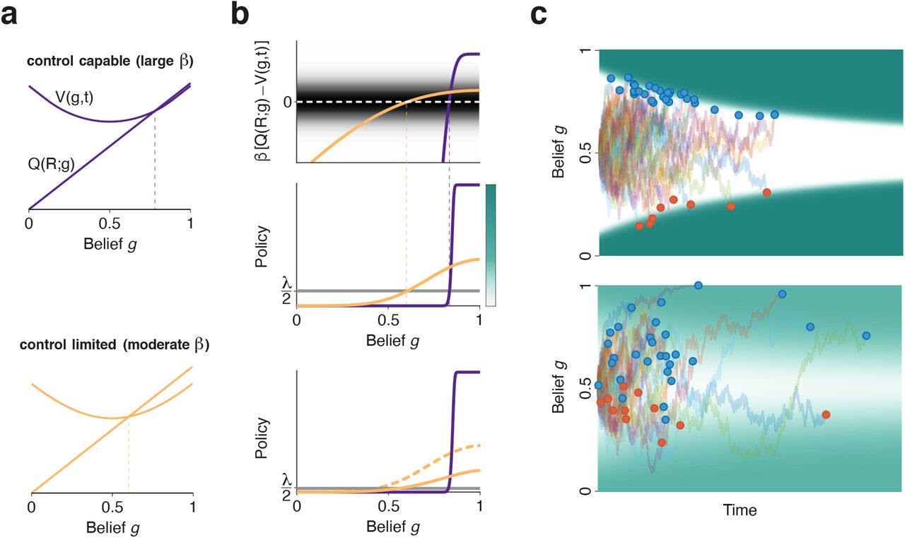
(a) Value function for waiting (convex curve) and action value for choosing R (straight line) as a function of belief at the beginning of the trial (t = 0), for a control capable (top) and a control-limited agent (bottom). Dashed lines indicate the belief for which both quantities are equal. (b) Top. Difference between the two curves in (a) for each agent (same color code as in (a)) scaled by the agent’s control ability β. Dark background signals the region where the scaled difference in action values is of order unity. The probability of committing to a choice varies over the range of beliefs for which the scaled difference overlaps with this region. Middle. Choice policies at this time for the two agents. Vertical dashed lines mark the transition from suppressing to promoting choice relative to the default policy Pd(R) = λ/2. (Bottom) Same as middle but for agents where the default response rate has been reduced by a factor of 4. For comparison, the policy for the control-limited agent in the panel above is also shown here as a dashed line. (c) Decision-making dynamics for control capable (top) and limited (bottom) agents, with the same default response rate λ as in (b), top. Traces are belief trajectories (Methods) for a set of trials with moderate strength of evidence towards the right (i.e., positive beliefs). Background represents the policy (instantaneous probabilities of choice commitment per unit time; see colorbar in (b), bottom, for the relative magnitudes of these probabilities). Dots signal the moment of commitment in each trial. See methods for parameters in this figure.
At each point in time, an agent that is well adapted to the task will choose between committing to either of the two possible options (which we describe as Left (L) and Right (R), with R being correct when the latent variable is positive), and continuing to sample the stimulus (i.e., ‘waiting’ (W), Fig. 1e) in order to make a more accurate choice later on. This embodies a speed-accuracy trade-off, which is the essential computational problem in perceptual decision-making11,13. We consider agents with default response policies that are not task-adapted, and which will thus need to exercise control in order to perform well. By default, agents have a certain constant probability of commitment λ per unit time and, when they do commit, select one of the two options randomly. These default policies describe agents with a propensity to lapse in all trials, with an exponential RT distribution of mean λ−1 s. For most of our results, we consider that binary choices under the default policy are unbiased (i.e., maximally unconstrained given the response rate λ), but in Fig. 8 we consider biased default policies in the context of history effects. The problem we describe can thus be cast as an agent trying to maximize reward given a limited ability to control a default tendency to lapse with a certain urgency throughout the trial.
Adaptive behavior in the task requires the agent to control these default policies in two ways. First, the tendency to respond needs to be matched to the requirements of the task. For instance, if the task emphasizes accuracy over speed but λ is large, control will have to be used to slow responding down. The magnitude of the parameter λ can thus be understood as biasing the agent towards or against speed in the speed-accuracy tradeoff defined by the requirements of the task. Second, the actual categorical choice needs to become stimulus-dependent. Indeed, adaptive policies will use the agent’s belief g(t) to update the probability of each of the three possible actions throughout the trial (Fig. 1e).
Optimal policies for control-limited agents consist of smooth decision bounds
Previous studies showed that, in the absence of control limitations, the optimal policy is for the agent to make a choice when its instantaneous belief g(t) reaches a certain time-dependent decaying bound14,15. This bound corresponds to the moment where the action-value of committing to either of the two options – which tends to grow through the trial – becomes equal to the initially larger long-term value of the uncommitted state – which decays (Supplementary Fig 1). Since this bound on belief corresponds to a bound on accumulated evidence (albeit with a different shape; Supplementary Fig. 1), the optimal policy has a neural implementation in terms of a drift-diffusion model14,15,42, as long as the temporal evolution of the decision bounds can be specified accurately.
In order to investigate optimal decision policies in control-limited agents, we extended the KL formalism to incorporate sensory uncertainty (partial observability) as well as a combination of continuous (for the agent’s belief) and discrete (for the agent’s actions) state spaces in continuous time (Supplementary Information). Our results show that optimal control-limited policies generalize naturally the policy just described: instead of transitioning discontinuously from waiting to responding, they are described by a temporally evolving probability of commitment which, for any fixed time, grows with the action-value of the two options relative to the value of the uncommitted state (Fig. 2), with the steepness of the transition growing with β. In fact, the optimal policy is given by a simple mathematical expression (Supplementary Information)

Here, Q(a; s) is the action-value of action a = R, L, W in state s = g, t, and V(s) is the long-term value of the uncommitted state. The exponential term provides a gain factor on the agent’s default probability of committing to either action per unit time Pd(R, L) = λ/2. The belief at which the action-value of commitment and the value of the uncommitted state become equal marks a transition from suppressing the default tendency to respond to augmenting it, with β measuring the steepness of this transition (Fig. 2b, top). In control-capable agents, the transition from low to high probability of commitment as a function of belief g(t) is sharp, and the probability per unit time in the high state is large (Fig. 2b, middle), effectively resembling a hard bound on g(t) (Fig. 2c, top). In contrast, the more control-limited an agent is, the more similar the commitment probabilities in the low and high states become, and the larger the range of beliefs over which the transition occurs (Fig. 2b, middle). For such agents, behavior is more stochastic and there are broad ranges of belief and time for which the agent can either be committed or uncommitted in different trials (Fig. 2c, bottom). When the default rate of responding λ of the agent changes – for instance, decreasing – the probability per unit time of commitment as a function of belief is scaled down, but only for control-limited agents (Fig. 2b, bottom). This is equivalent to a default emphasis on accuracy (over speed). Everything else kept equal, lower values of λ lead to longer RTs and thus better choices, although not necessarily larger reward rates, as we explain below. In sum, optimal decision policies for control-limited agents with lapsing default policies resemble smooth decision bounds. This is a form of noise-induced linearization, a common phenomenon which takes place in many physical systems, including neurons43.
The task stakes specify the behavior of the FAB agent
Before examining the effect of control limitations on the phenomenology of decision making, we consider a more general question, namely, how large is the space of possible optimal solutions to a sequential sampling decision problem? Although the problem as we have construed it depends on more than a handful of parameters (specifically seven: five for the task – the noise in the stimulus σ2, the width of the prior  , the reward magnitude Rw and penalty time tP, and the inter-trial-interval tITI – plus two for the agent – the control ability β and the default response rate λ) it can be shown that the task faced by the agent depends effectively on a single dimensionless parameter This parameter, which we refer to as the ‘stakes’, is given by S = (tP + tITI)/tg, i.e., the sum of the penalty time and the inter-trial interval relative to
  , which describes the intrinsic time-scale of the inference process. tg measures the time interval that it takes the agent to reduce its initial uncertainty about the strength of evidence in half by sampling the stimulus. Unless specifically noted, we always measure time in units of tg, which is the natural time-scale of the decision problem. Intuitively, when S ≫ 1, stimuli are presented rarely, so maximizing the reward rate demands that the agent samples the stimulus sufficiently long to make accurate choices, i.e., the stakes for the agent for performing well in the task are high. Conversely, when S ≪ 1, stimuli arrive so frequently that it becomes worthless for the agent to invest time in sampling the stimulus, as another opportunity will be presented soon in which reward can be obtained with at least 50% probability. Because the magnitude of the stakes determines in this fashion the optimal stimulus sampling time allocation, one can think of the stakes as quantitatively specifying the speed-accuracy demands associated to the task.
For the FAB agent (β−1 = 0), the optimal policy depends exclusively on the stakes4,44 (Fig. 3). It is instructive to understand this situation in detail, as sweeping the value of the stakes defines the whole universe of optimal solutions to the sequential sampling decision problem. The agent adapts its policy to the stakes of the task by raising the decision bound when accurate performance is needed (Fig. 3a). As this happens, both accuracy and RT naturally grow (Fig. 3b). Reaction time grows faster which, together with the larger interval between trials, results in a monotonic decrease of the reward rate of the policy with the stakes of the task (Fig. 3b, inset). The fact that agents solve the task by deciding how much time to allocate to each stimulus according to the background rate of stimulus presentation in the environment suggests interesting connections between perceptual decision making and foraging theory45.

All panels in this figure describe the behavior of the FAB agent (i.e., β−1 = 0). (a) Decision bounds on belief for three values of the stakes S (see text). (b) Left. Accuracy averaged across all difficulties (equal to the decision confidence (DC); see Methods) as a function of the task stakes S. Right. Same for RT. Inset. Reward rate decreases monotonically with S. The three values of S in (a) are marked with circles of corresponding colors in (b,c). (c) Relative difference in (average) RT between correct and error trials as a function S. (d) One to one map between instantaneous belief g and time and accumulated evidence during the trial (Methods). (e) Behavior of the agent for a low-stakes task. i. Decision bound on accumulated evidence. ii. Psychometric function. iii Chronometric functions for correct (blue) and error (red) trials. iv. DC as a function of evidence strength for both outcomes. In panels (ii – iv) the upper limit on the strength of evidence μ is twice the width σμ of the prior. (f,g) Same as (e) but for moderate and high stakes respectively. Insets in (iii, iv) show difference in RT and DC respectively between correct and error trials.
A number of quantitative signatures of behavior have been identified as useful for distinguishing between different mechanistic implementations of the decision making process. One of them is the difference in RT between correct and error trials46. This difference is non-monotonic in the task stakes, defining three qualitatively different regimes in this problem. For low enough stakes, it is negligible (Fig. 3c). For intermediate stakes, incorrect decisions take longer than correct ones, and for sufficiently high stakes this pattern is reversed. The reversal is a consequence of the shape of the map between accumulated evidence and belief g(t) (Fig. 3d, Supplementary Fig. 1). It is known that decaying bounds result in larger RTs for errors47. However, it is important to realize that the relevant bounds are those on accumulated evidence, not on belief. Although the bounds on belief always decay with time (Fig. 3a), extremely large values of accumulated evidence are necessary to reach large values of g(t), specially at long times (Fig. 3d), resulting in a situation where the optimal bounds on accumulated evidence initially grow with time when the stakes are sufficiently high (Fig. 3g). This mechanism also leads to an outcome-dependent reversal in decision confidence (Fig. 3e,g) as a function of the stakes. Empirically, the relationship between the RTs of correct and error trials is seen to vary with the specific conditions of the discrimination task8,48,49, as we discuss below (Fig. 6).
Decision making in control-limited agents
For control-limited agents, the task depends effectively both on the stakes and the inter-trial interval, although the phenomenology does not change qualitatively from this extra parameter. We generally fix tITI = tg and control the stakes S by manipulating the time penalty for errors tp (i.e., S = tp + 1). In addition, the optimal policy now depends also on the properties of the agent, both its default response rate λ as well as its capability for control β. In Fig. 4 we show how the main features of the behavior of the agent in the discrimination task depend on these three parameters. When the control ability β is sufficiently low, the agent behaves essentially according to the default policy. The mean RT is thus equal to λ−1 and accuracy is at chance level independently of the task stakes (Fig. 4a-b). At the other extreme, when β is sufficiently high, the agent’s behavior is unaffected by the default policy (Fig. 4a-b) and depends only on the stakes (Fig. 3). Accuracy is non-monotonic with β if the stakes are low and the agent is slow (small λ). This happens because accuracy initially increases as the agent becomes able to adapt its behavior to the task. Because this agent underemphasizes speed, its accuracy can grow to be quite high even for a moderate increase in β. However, because the stakes are low, the fully adaptive strategy is to forego of accuracy and decide quickly instead (Fig. 3b), leading to the non-monotonic behavior in Fig. 4b.

(a) RT (averaged across difficulties) as a function of the control ability of the agent β. Blue and orange represent agents with low and high default response rates, respectively. Dashed and solid lines represent tasks with high or low tp, respectively, which result in correspondingly high or low stakes (b-d) Same as (a) but for accuracy/decision confidence (b), reward rate ρ (c) and the total control cost (d) respectively. (e-f) Same four quantities, but plotted as a function of the penalty time tp for a moderately control-limited agent (β = 24). For comparison, in (e-g) the black dashed line shows the behavior of the FAB agent. Because we are fixing tg = 1, throughout this figure S = tp + 1.
The reward rate ρ always grows with the control ability β (Fig. 4c), confirming the intuition that control-limitations always represent a handicap for the agent. The monotonic relationship between β and the reward rate establishes an exploitable link between control and motivation30,50, which we address below (Fig. 6; Discussion). The total control cost, given by β−1KL[Po|Pd], is always zero for extreme values of the control ability. When β is close to zero, control is too costly for the agent, so the optimal strategy is to operate under the default policy, in which case the KL term vanishes. At the other extreme, when β−1 is near zero, the total control cost is zero because there are no control limitations. The control cost is maximal at intermediate values of β, and where this maximum is attained depends on both the agent’s default response tendencies and on the task stakes (Fig. 4d).
One can also look at the behavior of the agent as a function of the stakes when the control ability is fixed. This reveals explicitly that, compared to the FAB agent, the control-limited agent is not able to adapt its behavior to the demands of the task. For instance, when the stakes are very low, the mean RT of an agent which emphasizes speed  is close to optimal (i.e., similar to that of the FAB agent), because the task does not demand extended accumulation of evidence. But when the task stakes are high, the default impulsivity of this agent is clearly detrimental to performance (Fig. 4e-f). In contrast, a slow agent
  can have similar accuracy and RT as the FAB agent when the stakes are very high (Fig. 4e,f), since in those conditions its default RT is well-matched to the demands of the task. The delayed commitment of this agent allows it to actually outperform the FAB agent in terms of accuracy when the stakes are low (Fig. 4f), but the extra time invested does not pay off sufficiently, leading to a suboptimal reward rate in (Fig. 4g). Agents with different default commitment rates are closest to the FAB agent in terms of reward rate at different values of the task stakes (Fig. 4g). When the stakes tend to require RTs matched to the default commitment rate of an agent, the corresponding control costs under the optimal policy are smaller (Fig. 4h).
Signatures of control limitations on decision confidence
The smoothing of the decision bounds caused by the control-limitations of the agent (Fig. 2) strongly shapes the transformation from sensory evidence into categorical choices. In particular, limitations in control alter the beliefs of the agent at the moment of commitment, i.e., the agent’s decision confidence (DC). DC in a categorical choice measures the decision-maker’s belief in her choice being correct51,52. A research program within psychology and cognitive neuroscience has documented how explicit judgements (or implicit measures53) of DC depend on various properties of the decision problem, such as discrimination difficulty, trial outcome or time pressure51,54–56. Normative approaches have also explored the phenomenology of DC that follows from statistically optimal decision strategies57–59.
In order to systematically characterize how control-limitations shape DC, we examined the behavior of a control capable (β = 28) and a moderately control-limited (β = 23.5) agent for easy and difficult discriminations. In both discriminations the latent variable is positive (i.e., R is the correct choice), but we varied the strength of the evidence. We recall that g(t) describes the agent’s belief that the latent variable is positive. Thus, DC is given by the value of g(t) at the moment of commitment for rightward decisions, and by 1 – g(t) for leftward ones. When the strength of evidence is weak, individual trials are compatible with beliefs spanning both choice options depending on the stochastic evidence (Fig. 5a left), whereas when the strength of evidence is large, the agent’s beliefs quickly converge on rightward preferences (Fig. 5a right). We developed methods to compute semi-analytically the joint distribution of DC and RT corresponding to the optimal policy of any of our agents (Supplementary Information).

(a) Temporal evolution of belief for a difficult (left) and easy (right) stimulus conditions. The probability distribution of beliefs (Methods) is normalized at each time. (b) Left. Joint distribution of belief (at decision time) and RT for correct and error trials for the difficult condition (a, left) for a control capable agent (β = 28). Circles represent the mean. Line demarcates the region enclosing 90% of the probability mass. Right. Same but for the easy condition in (a, right). The means and regions of high probability from the hard condition are also shown for comparison. (c) Left. Mean belief at decision time as a function of the strength of evidence for correct and error trials. Circles show the values used in (a,b). Right. Decision confidence (equal to 1-g if g < 0.5) as a function of the strength of evidence. (d,e) Same as (b,c) but for a moderately control-limited agent (β = 23.5). (f) DC conditioned on RT as a function of outcome (left) and difficulty (right) for the control-capable (CC; top) and control-limited (CL: bottom) agents.
For control-capable agents, this distribution is tightly focused (Fig. 5b) around the regions where the probability of commitment abruptly transitions from zero to a large value (Fig. 2b,c), which approximates the policy of the FAB agent, based on a temporally decaying decision bound15 (Fig. 3). When the strength of evidence grows, the distribution still tracks the symmetric bounds but is shifted towards earlier RTs, and thus more extreme beliefs (Fig. 5b, right; Fig. 5c, left). Because the bounds are necessarily outcome-symmetric, DC is almost outcome-independent and grows with the strength of evidence (Fig. 5c, right). The outcome-dependence of DC is referred to as confidence resolution (CR)51,54,55. Interestingly, the optimal decision policy without control limitations, which is always superior in terms of reward rate, has poor CR. A tendency for decision confidence to increase with the strength of evidence regardless of outcome is sometimes observed57,60,61, specially in experiments requiring simultaneous reports of decision confidence and choice57,60 (Discussion).
For the control-limited agent, the joint distribution of DC and RT is much less concentrated (Fig. 5d; see also Fig. 2c). When the strength of evidence is almost zero, the distributions for correct and error trials are still approximately symmetric (Fig. 5d, left). But for easy conditions both distributions shift up towards rightward beliefs (i.e., towards the evidence), making them asymmetric with respect of outcome (Fig. 5d, right). Intuitively, this occurs because the control-limited policy, despite being outcome-symmetric, is less restrictive in terms of the values of belief and RT where commitment is possible, so when beliefs are strongly biased by the evidence, DC ends up also reflecting this bias (Fig. 5d, right, Fig. 5e, left). Since errors occur when the agent believes L is the correct choice (g < 0.5), the biasing of these beliefs by the evidence (towards R, i.e., towards g = 1) implies a more undecided state (g closer to 0.5), i.e., lower DC. This process results in opposing trends for DC as a function of the strength of evidence for correct and error trials (Fig 5e, right), demonstrating that optimal control-limited policies possess good CR. CR is generally observed in psychophysical experiments56,58,62–66, but had so far been unaccounted within a normative sequential sampling framework (see Discussion).
Control-capable agents have poor CR because, when choices are triggered by hard bounds on belief, the only quantity that can shape decision confidence is RT (through the time-dependence of the decision bounds). In fact, if the bounds were constant, as in the SPRT, decision confidence would be identical for all choices, as noted early on67. Thus, for agents using these kinds of policies, decision confidence conditional on RT is independent of any other aspect of the problem, such as trial outcome or strength of evidence (Fig. 5f, top). In contrast, decision confidence in control-limited agents is shaped by all factors that affect the beliefs of the agent before commitment, and is therefore larger for correct than error trials, and for easier compared to than harder conditions (Fig. 5f, bottom). In sum, the stochastic nature of commitment imposed by the control limitations of an agent provides a natural explanation for the coupling between DC and the underlying factors that shape the beliefs of an agent during a perceptual decision.
The control-limited regime
In addition to CR (Fig. 6a, left), control-limitations have signatures at the level of RT and also at the level of accuracy conditional on RT (i.e., time-dependent accuracy or TDA68, shown here averaged across difficulties). Errors following the control-limited policy are faster than correct choices (Fig. 6a, middle), as already evident in Fig. 5d. Errors tend to occur earlier because, on the one hand, the stochastic control-limited policy allows commitment with ambivalent beliefs and, on the other hand, these beliefs are more likely earlier on, as the belief of the agent aligns with the evidence as the trial progresses (Fig. 5a,d. Supplementary Fig. 2). In addition, TDA has a characteristic profile of initial growth and, if the control ability of the agent is low, it saturates to a roughly constant value (Fig. 6a, right). Qualitatively, these features are robust for control-limited agents, regardless of the specific β and λ of the agent (Fig. 6b). This is in contrast to the behavior of the FAB agent (or agents with very large β). As we showed in Fig. 3f, unless the stakes of the task are enormous, error RTs are longer than those of correct trials (although by a small amount. The hard bounds on accumulated evidence of the FAB policy decay relatively slowly, and this leads to a small outcome dependence of RT – Supplementary Fig. 1) and to a monotonically decaying TDA69.

(a) Example of outcome-dependence of DC and RT as a function of difficulty (showing clear CR and fast errors) and TDA, in the control-limited regime. (b) Magnitude of ΔDC/DC (which is equal to DCcorr - DCerr averaged across difficulties, relative to the same average regardless of outcome) and ΔRT/RT (same definition but for RT) in the space of β and λ. (c) Reward rate ρ as a function of the control ability β. Top and bottom show the same baseline situation, together with an estimated constant target reward rate, and the modified reward rate profiles under a change in the time penalty for errors tp (top; equivalent to a change in time-pressure) and the time-scale of inference tg (bottom; equivalent to a change in difficulty). (d) DC, RT and TDA (as in (a)) for the baseline situation (middle; signalled by a gray circle in (c, top)), a situation with a lower value of β that keeps the same target ρ under an increase in time-pressure (top; signalled by a light-gray circle in (c, top)), and a situation with a higher value of β that keeps the same target ρ under an increase in difficulty (bottom; signalled by a dark-gray circle in (c, bottom)).
These data show that it should be possible to identify control-limited behavior based on these features. A difficulty, however, is that it is not trivial to manipulate experimentally the contro-lability of a subject performing a discrimination task. Particularly in the case of human subjects, given instructions to perform, subjects will generally mobilize cognitive resources to comply. We reasoned that a strategy to find the control-limited regime would be to focus on situations where there is little incentive to invest resources in the task. First, we note that although so far we’ve treated the control ability β as a property of the subject, the ability to exercise control is both a dynamic and a limited resource28,70–72. Thus, it is expected that subjects will shape their allocation of control taking into account the gains they might experience from different allocation policies30,73. As we showed in Fig. 4, the reward rate of the agent increases monotonically with β. Thus, in principle, a reward-maximizing agent should seek to increase the amount of invested control. In practice, however, subjects are expected to use satisficing, rather than maximizing strategies74. Alternatively, the marginal utility of reward (rate) is expected to decrease when the agent is satisfied75,76.
We thus consider a realistic setting where an agent is performing a task whose parameters have been set so that the agent is close to the point of satisfaction using a certain amount of control (Fig. 6c). How is the agent expected to re-allocate control under different task manipulations? We considered two manipulations that are commonly used: changing time-pressure and changing the overall difficulty of the discrimination task. In our model, the time pressure is effectively controlled by the task stakes S (Figs. 3,4). Low stakes normatively induce time-pressure by effectively penalizing long RTs in terms of reward rate (Fig. 3). In practice, we lower the stakes by lowering the penalty time tp after an error. Difficulty is controlled by the inference time-scale tg. The lower tg, the shorter the time that it takes to identify the latent state on average, i.e., the easier the task. Decreasing the error penalty or decreasing the difficulty will both increase the reward rate of the agent, but if the agent is already close to its target reward rate, then the agent can stay at the target by using a lower β (Figs. 6c top, 6d bottom). Conversely, in response to the opposite manipulations, the agent should invest more control to stay at the target (Figs. 6c bottom, 6d top). Lower difficulties and time pressure are thus associated with control-limited phenotypes, whereas emphasis on accuracy and difficult discriminations correspond to control-capable behavior (Fig. 6d) These considerations suggest that control-limited behavior might be observed in conditions with high time pressure and easy discriminations. Indeed, this is in agreement with a substantial body of work in human decision making. Errors tend to be faster than correct trials under speed emphasis and in easy tasks8,64,77,78, but slower than corrects under accuracy emphasis and hard discriminations8,48,64,67,78. CR has also been described to increase with time pressure64,65. As far as we can tell, the effect of manipulations of difficulty or time-pressure on the TDA has not been quantified in human decision-making, and thus remains an untested prediction of our theory.
Previous studies have focussed on post-decisional processing as a mechanism for producing CR in a sequential sampling framework64–66,79. In this kind of models, choices are still triggered when the accumulated evidence hits a bound (hence, choice and RT phenomenology is not affected), but DC depends on evidence accumulation after a decision is made. Typically, confidence is assumed to be a function of the value of the decision variable at some fixed time after commitment, referred to as the inter-judgement time. Post-decisional processing naturally leads to CR64,80, and previous work has shown that CR indeed grows when the inter-judgement time is experimentally increased66,79. Thus, both post-decisional and control-limitations produce robust CR in a sequential sampling setting. The two mechanisms, however, are clearly distinct. A FAB agent using post-decisional processing for DC will have the same outcome of RT and TDA curve as the standard FAB agent. Thus, these behavioral signatures can be used to distinguish control-limitations from post-decisional processing.
Control limitations and decision lapses
During sensory discrimination experiments, lapses are identified by a saturation of the psychometric function to a value different from one or zero, signaling errors that don’t have a sensory origin. Since action-selection under the default policies we consider is stimulus-independent, it is expected that control-limited agents will lapse if their control ability is sufficiently low.
Indeed, the psychometric function of the control-limited agent starts showing lapses as β decreases (Fig. 7a,c). Lapses appear when the probability of committing to either option is still close to the default rate λ/2 even under complete certainty about the sign of the latent variable, i.e., for beliefs g = 0, 1 (Fig. 7b). Avoiding lapses requires being able to form the appropriate beliefs based on sensory evidence, and being able to act on the basis of those beliefs. The control-limited agents we model are capable of the former process, but may not be capable of the latter. As the control ability of the agent increases, response probability becomes more strongly dependent on its beliefs. In particular, the probability of a correct response under sensory certainty becomes large, and the corresponding error probability becomes zero, and lapses disappear (Fig. 6b).

(a) Psychometric functions display increasing lapse rates as the control-limitations of the agent grow (β = X,..,Y from orange to blue). (b) Decision policies as a function of belief (at time t =X) for two of the agents in (a) (same color scheme). The black horizontal line represents the default stimulus-independent policy. (c) Lapse rate as a function of the control ability β and default response rate λ. (d) Psychometric functions for a control-limited agent (β =X and λ =Y; black), its standard correction (green; obtained by simply scaling the black curve until its asymptote reaches 1), and the correction obtained by setting β−1 = 0 (red; which is the (optimal) psychometric function of the FAB agent). (e) Same as (d) but for an agent for a fast default response rate λ =X. (f) Ratio between the slope of the psychometric function corrected with the standard method and the psychometric function of the FAB agent, as a function of β and λ. At the dashed plane both corrections agree. The two circles show the examples in (d) and (e). (g) Psychometric functions in a ‘single sensory sample’ model (equivalent to a SDT setting) as a function of the control ability of the agent (Methods). (h) Lapse rate (blue) and ratio between the slopes of the two corrected psychometric functions (same as (f)) for this model.
In most psychophysical experiments, one uses behavior to infer the sensory limitations of a subject, for instance through the slope of the psychometric function at the categorization boundary. Because lapses change the shape of the psychometric function, they obscure the true psychophysical abilities of a subject. Developing methods to recover sensory limitations in the presence of other, non-sensory, processes shaping behavior, has been a critical problem in the history of psychophysics which, for instance, gave rise to the development of Signal Detection Theory81 (SDT). The standard approach to recover a ‘clean’ estimate of stimulus discriminability in the presence of lapses is simply to scale up the slope of the psychometric function until its asymptotes reaches one and zero82. This is appropriate when lapses reflect inattention83. On the other hand, when lapses result from control limitations, the proper approach to recover the true sensory limitations of the agent is to examine their psychometric function at β−1 = 0, i.e., in the absence of any limitations in control. To compare the performance of both approaches, we considered the result of applying both types of corrections to the psychometric function of a control-limited agent. Interestingly, the two approaches don’t, in general, coincide (Fig. 7d-f). In fact, the ‘cleaned’ psychometric slope obtained using the standard approach can either over- or under-estimate the slope of the psychometric function of the FAB agent, depending mainly on the default response rate λ (Fig. 7f). Consider the case of an agent whose control-limitations produce a significant lapse rate (Fig. 7d-e). Small values of λ describe situations where the default time to respond is long compared to time-scale tg of the inference process. In this case, the default policy of the agent overemphasizes accuracy over speed, leading to a steeper psychometric function compared to the FAB agent (at the cost of a lower reward rate). In these conditions, the standard correction overestimates the optimal psychometric slope (Fig. 7d). In contrast, when λ is large, the suboptimal reward rate of the control-limited agent comes from overemphasis of speed over accuracy, and this is associated to an underestimation of the optimal psychometric slope by the standard correction (Fig. 7e).
The discrepancy between the two correction methods is still there when one considers a simpler decision problem where an agent only receives one sample of sensory evidence (equivalent to a SDT setting). Here, one can also define optimal control-limited policies which will display lapses if the control ability of the subject is sufficiently low (Fig 7g; such policies are mathematically equivalent to those in Pisupati et al.83, but see Discussion). In this setting, the pure ‘sensory-limited’ psychometric function does not depend on speed-accuracy considerations, and the standard correction factor always underestimates the true psychometric slope (Fig. 7h). Furthermore, comparing the lapse rate of the agent and the correction factor as the control ability of the agent grows, it is apparent that the correction factor still underestimates by the time the lapse rate reaches zero (a feature also present in the sequential decision problem, i.e., compare Fig. 7c and Fig. 7f at β ~ 22.5). This implies that saturation of the psychometric function to 1 or 0 does not automatically guarantee that the psychometric slope reflects the agent’s true sensory limitations (Discussion).
In summary, control limitations naturally lead to lapses in decision-making. Our results show that the proper correction to the observed psychometric function depends on how lapses are generated, that the standard correction is in general not correct when lapses are due to control limitations, and that corrections might still be needed even if lapses are not fully apparent.
Sequential dependencies and decision biases
In laboratory settings, where many decisions are performed during an experiment, it is often observed that behavior in one trial can be partly explained by events taking place in past trials24,25,84–86. Many different forms of such sequential dependencies have been described, reflecting different processes including, for instance, reinforcement learning85 or bayesian inference84. Whereas sequential dependencies are often (but not always84) maladaptive within the short term context of the task, they are typically adaptive when one considers longer-term environmental regularities. Such situations, where the short-term context and the long-term environment have opposing demands, are exactly the ones benefitting from control, which suggests that control-limitations might provide a natural framework for describing some forms of sequential dependency.
At a mechanistic level, most forms of sequential dependencies can be grouped into three classes, according to the quantity that is updated from one trial to the next. One class corresponds to updating the predisposition of choosing an action before the stimulus is observed, which can be modelled using biased default response policies (Fig. 8a-c). Another class corresponds to updating the value of the different actions, depending on previous events (Fig. 8d-f). A third class corresponds to updating the map that links sensory evidence to the belief that a given action is correct. Within our framework this can either correspond to updating the prior beliefs of the agent about the latent state before stimulus onset, or the decision criterion that determines which values of the latent variable map to each action (Fig. 8g-i). We devised a procedure for deriving optimal policies that incorporate each of these three forms of trial-to-trial updating (Supplementary Information). Importantly, each class can be used to describe a number of qualitatively different sources of sequential dependence. For instance, updates in the default probability of choosing an action can depend on the previous choice, or on an interaction between the previous choice and outcome. Our grouping into classes thus reflects the target of the cross-trial updating, not the events that cause the update.

(a) Schematic description of a class of sequential dependencies where previous trials lead to a bias in the default action policy, depicted as a shading over one of the actions in the current trial (b) Three scenarios where the default policy is unbiased (black) or biased towards action R (blue) or L (red; Methods). (c) Psychometric functions for each of the three cases in (b) for control-limited (left) and control-capable (right) agents. (d) Similar to (a), but where trial history shapes the current value of the action that the agent just performed. (e) Three scenarios where the agent choose R in the previous trial and the history of choice-outcomes experienced leads to the reward magnitude in the current trial being modelled as higher (blue), lower (red) or average (black). (f) Same as (c) for value biases. (g) Similar to (a) but where trial history shapes the agent’s prior beliefs about the upcoming stimulus, depicted as a shading over one of the stimulus categories before the vertical bar marking stimulus onset. (h) Three scenarios where the agent believes the latent variable in the current trial is more likely to be positive (blue), negative (red) or is unbiased (black). (i) Same as (c) but for biases in stimulus probability.
To reveal the effects of these different forms of sequential dependence, we plot the psychometric functions of the agent conditioned on the relevant event in the previous trial. We use as a baseline an agent whose control limitations lead to a substantial lapse rate, and then show how the effect of each form of sequential dependence on the psychometric function is modified as the agent becomes control-capable. This strategy helps evaluate how control limitations shape the pattern of sequential dependencies in each class. The signature of sequentially updating the bias of the default policy, is a symmetric vertical displacement in the psychometric function87 (Fig. 8c, left). This is because increasing the probability of one action automatically implies lowering the probability of the other. These vertical shifts are unoccluded when the psychometric function does not saturate to one or zero, which is the case if the agent is sufficiently control limited to show lapses. Because sequential biases reflect the default action policy, they disappear under conditions of high control (Fig. 8c, right).
Agents might, on the other hand, use their history of successes and failures to sequentially update the value of each action (Fig. 8d), instead of the default probability of choosing it. In experiments where rewards and penalties are fixed, this would be a form of suboptimality, but it might be expected if subjects have the wrong model for the task, and incorrectly attribute fluctuations in average value across trials (due to variable proportions of incorrect choices) to fluctuations in the single-trial value of an action88. Because only the value of the action that was just produced is updated (Fig. 8e), this type of sequential dependencies lead to asymmetric modulations of the psychometric function, in which the amount of bias is proportional to the likelihood of repeating the action (Fig. 8f, left), as was recently observed83. In this case, although the sequential bias is still there for control capable agents, the marked asymmetry is almost completely eliminated (Fig. 8e, right), because the probability of repeating the action is already saturated at its maximum value of 1 when lapses disappear.
A final scenario we consider is an update in the prior belief of the agent about the stimulus (Fig. 8g-h) which might arise, for instance, if there are across-trial correlations in the value of the latent variable which the agent is learning86. Typically, updating of stimulus priors is expected to lead to horizontal displacements in the psychometric function (Fig. 8i, left). For a given magnitude of the bias in probability (Figs. 8b,h), the changes to the psychometric function are smaller when the updated probabilities refer to the stimulus prior compared to the case when they reflect the passive action policy (compare Figs. 8c,i left). This is because the behavior of control limited agents is only weakly adapted to the task demands and reflects to a large extent their passive policies. Thus, because for this class of sequential dependencies, choice biases are adaptive, they grow with the control abilities of the agent (Fig. 8i, right). We conclude that the shape of the modifications in the psychometric function due to trial history, together with their dependency on the agent’s control ability, can be used to infer which aspect of the decision-making process is being updated across trials.
Discussion
We have systematically characterized how to optimally trade-off control and performance costs in perceptual decision making. We have considered stimulus-independent default policies to highlight the need for control in order to achieve good performance. Our default policies were also stochastic, as a means of phenomenologically describing all task-independent influences that might result in specific choices made at specific times. This type of default behavior results in optimal policies that have the form of smooth decision bounds. This means that there is no deterministic decision rule specifying when commitment will happen. Instead, accumulated evidence controls the probability of commitment, which transitions in general from a zero (or low) state, to a high state as the evidence favors more clearly one of the options (Fig. 2). Although our model is not mechanistic, in principle, an approximation of the control-limited policies we have found is compatible with a standard deterministic decision bound if one assumes that the true decision variable is a weighted sum of the belief-dependent decision variable x(g, t) we have described (Supplementary Fig. 1; Supplementary Information), and a stimulus independent stochastic term, which would induce stochasticity in the transformation from x(g, t) to action. The relative weight of these two components of the decision variable would be determined by the control ability of the agent. Control-capable agents would be able to suppress task-independent sources of input to the decision variable of the problem. A stochastic additive contribution to the decision variable can also be qualitatively approximated by trial-to-trial variability of a deterministic within-trial decision bound. This form of trial-to-trial variability has been considered in the past8, and gives rise to phenomenology which is qualitatively similar to the optimal control-limited policies. Our results can thus be interpreted as providing a normative grounding for this type of trial-to-trial variability in terms of control limitations.
Control-limitations robustly shape the phenomenology of decision making. One consequence of making decisions using probabilistic decision bounds is that it automatically results in good confidence resolution (CR; Figs. 5–6). CR arises naturally in normative models of decision making based on signal detection theory58,59,89 (SDT). But these models – which correspond in a sequential sampling setting to the use of vertical decision bounds – are clearly suboptimal when sensory evidence arrives in time, and are unable to account for the speed accuracy trade-off. However, at the cost of giving up on explaining RT, models with vertical decision bounds allow the decision variable at the moment of commitment to be sensitive to the way in which sensory evidence shapes the belief distribution, which is fundamentally what CR necessitates (Fig. 5). On the other hand, somewhat counterintuitively, the fully control-capable FAB agent of the sequential sampling framework has poor CR14,90 (Figs 3,5). Although being more confident in one’s knowledge when it is in fact correct seems advantageous, specially in a social setting91, it turns out that it is not optimal from the point of view of maximizing performance. In the absence of control limitations, choices should be made only based on instantaneous belief and elapsed time15,57, and thus outcome can only affect DC through its effect on RT (Figs. 3,5).
Given the widespread empirical observation of CR55,62,67, decision theorists have sought ways of obtaining robust CR within a sequential sampling setting. The standard solution relies on post-decisional processing of DC56,64–66,79. Separating in time decision commitment and DC permits using (effectively) horizontal bounds for choice while keeping vertical bounds (a la STD) for computing DC, which produces both speed-accuracy trade-offs and CR. CR has been shown to vary when the window of post-decisional integration is causally manipulated66,79, and at the same time lower CR is observed when choice and decision confidence are reported simultaneously by design57,60, suggesting that post-decisional integration does contribute to observed CR. Is post-decisional processing adaptive? There is conflicting evidence on this issue. Some work has pointed out to a need for post-decisional time to explicitly compute DC under some conditions56, and there are suggestions that some frontal areas as specifically involved in the computation of DC. At the same time, Bayesian confidence is an instantaneous function of accumulated evidence and elapsed time15,57,69, confidence and choice can be reported simultaneously57,60,66, and both choice and confidence-related signals have been observed in the same parietal circuits92–94.
Although control-limited policies and post-decisional processing both produce CR robustly, they are clearly distinct, and result in opposing trends in terms of the outcome-dependence of RT and of the TDA profile, quantities which are unmodified by post-decisional processing. Unless the stakes of the task are extremely high, the outcome-dependence of RT reverses sign as a function of β (Figs 3, 6). Such sign-reversal is well documented empirically: errors tend to be faster than correct trials in task settings which encourage speeded responding and where discriminations are easy8,64,77,78, whereas when the task emphasizes accuracy and for more difficult discriminations, it is correct trials that tend to have shorter RTs8,48,64,67,78. Our results suggest a normative explanation for this organization in terms of the connection between motivation and control: faced with the choice between continuing to invest control to increase reward with little marginal utility, and investing less control with little loss in satisfaction, agents will choose the latter (Fig. 6c). Our results predict that the shape of the TDA curve should change in parallel with the outcome dependence of RT (Fig. 6d). As far as we can tell this prediction has not yet been tested.
The previous argument depends on the assumption that the total availability of control is a limited resource. In behavioral economics, this is known as ego depletion28,70–72. The main finding is that subjects perform worse in a task requiring cognitive control after having participated in a previous cognitively demanding task (compared to controls). It is controversial whether the origin of this limitation has a computational origin73,95 or whether it is the consequence of scarcity of a physical resource28,95–97, but regardless of its mechanistic origin, an agent that is aware of this limitation should attempt to allocate the control expenditure in an advantageous way, in essence solving the hierarchical problem of optimizing task performance and control allocation simultaneously30. The dynamic allocation of control also seems relevant to describe variations in the level of engagement experienced by rodents during behavioral sessions in perceptual discrimination experiments. Recent studies98 have used hidden Markov models to identify transitions between states characterized by different levels of engagement, and shown that this phenomenology accurately describes some types of decision lapses and some forms of sequential dependencies. A more accurate description of the dynamic allocation of control would be useful to provide a normative understanding of this phenomenology, in particular what triggers these transitions, or even the very existence of discrete behavioral states. In our study, we also considered sequential dependencies, but focused on whether it would be possible to identify the targets of cross-trial modification based on the relationships they induce between the psychometric functions calculated in successive trials (Fig. 8c,f,i). We showed that sequential changes in action priors, stimulus priors, or action-values are dissociable, specially for control-limited agents. Interestingly, the three corresponding patterns of change in the psychometric function have all been observed experimentally in different tasks83,86,87.
We have shown that there is a natural connection between decision lapses and the ability to control task-independent default policies (Fig. 7a-c). Lapses arising from control limitations are formally similar to lapses construed as a form of exploration, as recently suggested by Pisupati et al83. However, whereas we view lapses as essentially reflecting a limitation of the agent, Pisupati et al. construe them as adaptive in perceptual decision-making tasks – because the agent will perceive action-outcome as being stochastic due to errors caused by their sensory limitations. We think it’s unlikely that the existence of sensory errors per se will generally be modelled by subjects, including rodents, as reflecting probabilistic reward contingencies, given that rats in some difficult perceptual decision-making tasks do not lapse3. However, exploratory strategies would be adaptive if the agent feels like it has not yet learned the correct model of the environment39, particularly at early stages of training. While it is possible that in some experiments, rodents (incorrectly) model the environment as perpetually changing – and thus sustain a stationary lapsing policy – we suggest that it might be reasonable to interpret this as a limitation to suppress a default tendency towards exploration. Independently of their interpretation, lapses obscure the true psychophysical performance of the agent. We suggested that the necessary correction when lapses reflect control limitations (or exploration) is in general different from the standard correction used in psychophysics82,83. The relationship between the two corrections depends on the speed, or accuracy emphasis imposed by the agent’s default policy (Fig. 7d-f), but the two are still different even for SDT models (Fig. 7g,h). In fact, our results show that the slope of the psychometric function will not, in general, reflect the true sensory abilities of the subject even if the psychometric function saturates to one or zero (Fig. 7f,h). This implies that accurate assessments of sensory sensitivity require paying attention to the functional form of the psychometric function, i.e., not all sigmoidal functions are equally appropriate.
Our framework assumes that agents attempt to control, given their ability, a default policy towards exploration. What exactly is the relationship between exploration and control? In the context of the exploration-exploitation trade-off, which is usually studied using n-armed bandit tasks39,99–101, some studies have suggested that, in fact, it is exploitation that should be considered as an automatic default, and that exploratory choices require cognitive control99. For instance, behavior driven by Pavlovian associations might be construed as automatic. However, a recent study with human subjects challenged this view, showing that conditions of high cognitive load (presumably making it more difficult for subjects to use cognitive control) result in a decrease of directed, not random, exploration. Both random exploration and exploitation increased in conditions of low cognitive load102. We would note, also, that exploitative behavior in an n-armed bandit task is very different from what constitutes exploitative behavior in a perceptual decision-making task, which requires temporal accumulation of evidence. Evidence accumulation is a form of working memory, expected to require cognitive control103. We also expect the default status of random exploration to be species dependent. To the extent that exploration might be adaptive during learning of a good causal model of the environment (see above), species less adept at causal learning might rely on exploratory behavior by default to a larger extent.
Code Availability
Custom MATLAB scripts used to implement the mathematical framework and produce the figures are available upon request.
Author contributions
J.C and A.R. conceived the project and the theory. J.C developed the theory and conducted the analysis. A.R. wrote the manuscript with feedback from all authors.
Competing Interests
All authors declare no competing interests.
Supplementary Figures
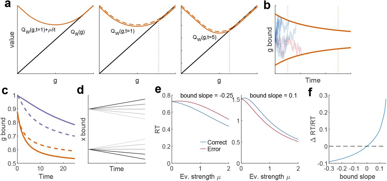
(a) Left: In black, action value of rightward choice as a function of belief g. In orange, action value of waiting for time t = 1 (a.u.), without considering the opportunity cost ρ · δt. The orange curve is tangent to the black one, as the information gained by waiting cannot decrease the value. Middle: When considering now the opportunity cost of waiting (new solid line, previous curve is now dashed), the action values of choosing right and waiting intersect at the optimal decision bound in belief for that time (dotted line). Right: Same as middle but for a larger time value (t = 5), notice that the bound has decreased. (b) Optimal decision bounds on belief as a function of time. A few example trajectories are shown (blue for rightward choices, red for leftward choices). The values of time used in (a) are marked by the vertical dotted lines. (c) In solid lines, same decision bounds in belief as in Fig. 3a (excluding the lower value of the stakes). The orange bound is also the same shown in (b). In dashed lines, belief bounds that would be obtained if the bounds in the accumulated evidence x were constant and equal to their value at t=0. For the orange case, the dashed curve is above the solid one, suggesting that the real bounds in x are decreasing in time, while for the purple case, the dashed curve is below the solid one, suggesting that the real bounds in x are increasing in time. (d) In order to capture the qualitative difference in the RT conditioned on outcome (ΔRT/RT = (RTcor – RTerr)/RTtotal) observed in Fig. 3c, we considered a minimal model where the decision bounds in x are linear with variable slope and fixed intercept (i.e. same value at t = 0), such that the bounds can either be increasing or decreasing in time. (e) Two examples are shown for the mean RT of correct and error responses for different signs of the bound’s slope. Left: example with negative slope, for which the RT of errors is larger than the RT for corrects. Right: example with positive slope, for which the RT of corrects is larger than the RT of errors. (f) plotting ΔRT/RT as a function of the bound slope reveals that a change in the sign of the latter is sufficient to induce a change in the sign of former, and that there is a one-to-one relationship between the two quantities. Interestingly, the relationship is highly non-linear.

(a) Example of a constant rate policy (homogenous poisson race) as a function of the accumulated evidence x, with the parameter b determining the sum of the rightward (blue) and leftward rates (orange), and a determining the difference between them. (b) RTD produced by two constant rate policies with different values of b. The distributions are the same for rightward or leftward choices. (c) As a consequence, mean RTs only depend on b (E[RT] = 1/2b), as shown plotted as a function of a. (d) conversely, the proportion of rightward choices only depends on a (P(R) = (1 + a)/2), as shown plotted as a function of b. (e) example trials visually demonstrating the results in (b-d). Top panels show rightward choices, bottom show leftward choices. In each column, the resulting RTDs are the same irrespective of choice. From the first to the second column, only b changes, so the choices overall become slower but the rightward proportion does not change. From the second to the third column, only a changes, so the RTDs stay the same but the rightward proportion changes. (f) Example of a simple monotonic rate policy: the rates are step functions of the accumulated evidence x, parametrized in the same way as before. As x changes sign, the rightward rate transitions from low to high, and the leftward rate does the opposite. The sum of both rates is still constant and only depends on b. (g) Distribution of x as a function of time for evidence strength μ = 1. Several quantiles are shown. (h) As the mass of the distribution of x shifts towards positive values with time, the conditional probability of a rightward choice increases and the conditional probability of a leftward choice decreases. Increasing μ (solid vs dotted lines) changes the speed of convergence towards the asymptotic values, which are still (1 ± a)/2. (i) This causes the RTDs for rightward and leftward choices to be different, as they are the product of the probability of making a choice at a given time (which still only depends on b and it is the same as in (b)) times the conditional probability of a given outcome (h). μ = 1 in this example. (j) Mean RT conditioned on choice as a function of evidence strength (in log scale). The mean total RT is always the same because it only depends on b, but it differs conditioned on outcome as the evidence strength controls the shape of the curves in (h). Throughtout this example (h-j), a = 0.6 and b = 0.5.
Supplementary Note
Here we present the mathematical derivation of our framework. To make the document self-contained, we include some theoretical background when needed.
1 Framework
1.1 Markov Decision Processes: First exit formulation
We consider a Markov Decision Process17,33,40 (MDP) with a set of states s ∈ S and a set of admissible actions a ∈ A. The actions generate transitions between states according to a transition probability T(s′|s, a) which crucially is Markov in the states and actions. Associated to each transition, there is an immediate reward  . The goal of the agent is to maximize the long term reward accumulated over the entire sequence of transitions. In order to do this, the agent is equipped with a control policy u(a|s), i.e., a decision rule to select actions in each state. The problem is then to find the optimal policy that ensures the largest possible long term reward.
In the ”first-exit” formulation of the problem33,40, there is a set ST ∈ S of “terminal” states which, once reached, terminate the process. The accumulated reward starting from state s and acting optimally thereafter, called the value function Y(s), can be written as
 where
where  is the reward obtained at time t having started from state s and following the policy, and the expectation is taken over any stochasticity in the process. tf denotes the time step at which the first terminal state is reached (which is also a random variable). The value function follows a recursive relationship called the Bellman Equation33,104 (BE), which is given by

It can be shown that if the immediate cost  does not depend on u, the optimal policy must be deterministic17 and given by
 which allows rewriting the equation (6) as

1.2 Kullback-Leibler control
In the above formulation of the problem, standard in the field of Reinforcement Learning, there are no costs associated to the control of the agent. In the field of Optimal Control, two reasonable features are added: First, it is assumed that the agent is capable of behaving in the absence of control. Second, it is assumed that control is costly, and that this cost should be included in the optimization process. Formalizing this idea means considering two policies. One is a control-free default (or passive) policy p(a|s), which describes the behavior of the agent in the absence of control and which, in principle, bears no particular relationship to the goals of the agent. This passive policy is part of the specification of the problem and plays a role similar to that of the prior in statistical inference. The other one is the target optimal policy u(a|s) which describes the trade-off between long-term reward maximization and control costs.
The framework of KL control32–34,37,105 assumes a specific form for the cost of control, which is added to the immediate reward  . The immediate consequence of choosing action a in state s under the optimal policy u(a|s) for an agent with default policy p(a|s) thus becomes

The constant β−1 measures the magnitude of the cost of control relative to the immediate reward, and can be considered a property of the agent. As we will see, when the cost of control is negligible (i.e., β → ∞), the attainment of long term reward dominates the behavior of the agent, and the optimal policy becomes identical to the one obtained in the standard MDP framework. However, when control is costly, the optimal behavior of the agent will tend to be constrained by its passive policy. Replacing  by
by  in the BE (8) one obtains
 where KL(p||q) is the Kullback-Leibler divergence38 between distributions p(x) and q(x), which gives its name to this framework. Thus, the effective consequence of the control cost is to penalize the optimal policy by a quantity proportional to the dissimilarity between the two policies, as reasonably expected. The usefulness of this formulation can be appreciated when applying some further algebra on the above equation:
 where the “partition function” Z(s) is defined as

The control law results trivially from the minimization of the KL divergence, which is attained when its two arguments are equal, resulting in KL = 0. In this case, the BE reduces to
 which is a self-consistency equation that specifies the value function. At the same time, the optimal policy is given by (from the condition KL = 0)

The last two equations (the equivalent of equations (8) and (7) above for the standard MDP) provide the solution to the KL control problem. It entails two important simplifications: First, unlike Eq. (8), Eq. (12) does not have a maxa operator and it is thus continuous. Second, once the value function in Eq. (12) is known, Eq. (13) provides an analytical expression for the optimal policy. This expression, furthermore, has an intuitive interpretation. Except for the normalization constant Z(s), the (un-normalized) optimal probability of choosing each action under the optimal policy uu(a| s) is proportional to the same probability under the passive policy p(a|s), with a proportionality constant that grows exponentially the net “action value” of the pair (a, s). One important consequence of this fact is that actions that have zero probability of being chosen under the default policy remain forbidden for the optimal agent. Thus, in KL control, control can only bias the probability of actions that were possible by default, it cannot create new actions de novo. This limitation can be seen as a price to pay for the mathematical simplification associated to the choice of the KL divergence as a measure of control cost.
1.3 Equivalence between MDP and KL formulations
Equations (12) and (13) are instances of the functions LogSumExp and SoftMax respectively

These are smooth versions of the max and argmax operators correspondingly. Notice that knowing the value of the first one facilitates the calculation of the second one, as it is the logarithm of the denominator. Expanding Z(s) in both (13) and (12)

 where we have defined the vector
  with components

Each Qa(s) measures the action value of being in state s and performing action a including a measure of control given by the surprisal log(p(a|s)). Since this is an immediate cost, it is useful to include it in the immediate reward, which we thus redefine to be

The second term is always negative, i.e., a cost. Thus, the more unlikely an action is in a particular state under the default policy, the lower the effective immediate reward in that state. This can be construed as a form of directed exploration towards the default. Using this modified effective immediate reward leads to the following natural expression for net action value Qa(s)

It’s straightforward to show that in the limit where β goes to infinity,  , and
, and  , so that the value function and the policy converge to the MDP deterministic solution in Eqs. (7–8).

1.4 Averaged-Adjusted Reward formulation
The first-exit formulation describes well a single trial in a decision making experiment, starting with stimulus onset and ending when the subject commits. However, a behavioral session contains many such trials, and requires a longer horizon. The standard way to deal with long (infinite) horizons is to use discounted rewards17. However, if the MDP is ergodic, there exists another approach which is well suited for describing a multi-trial decision-making experiment: reward rate maximization40,41. We explain this framework for a standard MDP, and later on show that it is trivially generalized to the KL control framework.
Let the MDP be represented by a discrete time, ergodic Markov chain40. We focus on the case where trajectories along the chain can be broken down in “trials”, with the beginning of each trial marked by the moment in which a certain initial state SI is visited. SI should be understood as a reference state, and the ergodicity of the chain allows us to make this choice arbitrarily.
Let us define
 with the same interpretation as in (5) except that N is a fixed and sufficiently large natural number, and where we have omitted the explicit dependence of the sequence of rewards on the policy (we in general assume the optimal policy). Since the state SI is always revisited, we can rewrite the equation separating it in two terms: one that captures the accumulated reward starting from state s until SI is reached for the first time, and another one capturing the remainder of the accumulated value since the first time SI is visited
 where kl corresponds to the successive times that the state SI is revisited, and the index l goes over trials, which go up to M. The conditioning on skl = SI makes explicit that every trial is initiated at the state SI. Only the first term depends on the particular initial state s at time t = 0, while the second term is independent of s and linear in M. This is equivalent to separating the initial (in)finite horizon problem into an initial first-exit problem, and a reduced (in)finite horizon problem that consists of a collection of identical first exit problems.
The reward rate ρ is defined as

Since the chain is ergodic, the reward rate for any policy is constant and independent of the initial state, so we can choose s = SI. We can employ the same sort of separation of N into trials that we did above. Multiplying and diving by M in both numerator and denominator we obtain

The expectation in the numerator corresponds to the average cumulative reward in one trial, while the expectation in the denominator corresponds to the average duration of a trial. Let us call these  and 〈T〉 respectively. Then we can simply write

The reward rate ρ is also defined as the gain of the policy, since it measures the slope of the asymptotic linear dependence of total reward with the duration of the trajectory. Policies that obtain differences in total future reward which are constant as N grows will all have the same ρ, but it would be desirable to know which policies maximize these finite contributions as well. The relative value, or bias, V(s) of the policy, defined as
 measures exactly this finite contribution, and is thus dependent on the initial state s. It can be shown40,41 that a policy that maximizes the relative value V(s) also automatically maximizes the reward rate ρ. In a multi-trial decision problem, V(s) can be written as

The expectation in the third term corresponds to  as we saw above, so that
 where the last equality uses the definition of ρ in Eq. (20). We now write the BE for the value function, taking the limit of N to infinity
 which, recalling that
  , and that YM is a constant independent of s, becomes

Using Eq. (23), this can be turned into a BE for the relative value V(s)

The last term uses the fact that the expected first exit time following a transition is exactly one unit less than the expected time before the transition, i.e.,

Since the expectation in this equation is already over trajectories obtained using the optimal policy, it can be taken outside the max operator, which leads to

We have thus transformed an infinite horizon problem on Y into a first exit problem on V, with the additional constant ρ in the left hand side. Although V(s) is a relative value, we will refer to it as the value function from now on. The value of ρ is unknown, but we know it has to satisfy Equation (23). This implies that V(SI) needs to satisfy the following condition
 since SI marks the start of a trial, the first term is the expected reward during one trial,
  , and the expectation in the second term is equivalent to the average duration of one trial, 〈T〉. Thus

In practice, this equation is used to obtain the value of ρ self-consistently: We solve the BE (26) for a fixed value of ρ, use it to evaluate V(SI), and repeat this procedure adjusting ρ iteratively until V(SI) = 0. The value of ρ for which this condition is met is the average reward rate of the policy.
Notice that, mathematically, the BE (26) is identical to the BE for a first-exit problem with a “cost of time” ρ, i.e., a problem with an immediate reward for each (s, a) equal to  . Such BE is well defined for any arbitrary ρ. It is only if one wants to interpret V(s) as the relative value of an infinite horizon problem with asymptotic reward rate ρ that Eq. (27) needs to be satisfied.
Finally, because no assumptions have been made on the form of the immediate reward, the average-adjusted reward formulation for KL control is trivially obtained replacing  in the previous equations by Equation (9). The relevant expressions become

1.5 Partial Observability: POMDPs
So far, we have been assuming that the agent has perfect knowledge about the states of the environment. In perceptual decision-making tasks, however, the challenge faced by the agent is precisely that the relevant states of the environment from the point of view of reinforcement are not directly observable, and have to be inferred through inference, based on stochastic observations. The appropriate mathematical framework to describe these situations is that of partially-observable Markov decision processes18,106 (POMDPs).
Qualitatively, this introduces the need for “information seeking” actions. In the problem we describe in the text, this action corresponds to the postponement of commitment, or waiting (which we have denoted by W). Although accumulation of evidence across time would seem to require memory and thus violation of the Markov assumption, it can be shown that the probabilistic belief of the agent (i.e., the posterior probability of the states given the full history of observations) can be updated recursively in a Markovian fashion, i.e., the agent’s belief in the current time-step is only a function of the current observation and the belief in the previous time-step18,107. Thus, formally, a POMDP can be construed as an MDP where states are replaced by beliefs18. If one uses the notation b = b(s1), …, b(sNs) to refer to the relevant beliefs of the agent over the states s, then the POMDP formulation of our problem is very similar to the one we have previously described


In this case, the immediate rewards  now correspond to the expected reward by the agent given its current beliefs. The quantity T(b′|b,a) replaces the transition probability T(s′|s, a) and describes the dynamics of belief induced by the dynamics of the agent-environment. Writing it in this form requires a marginalization over the observations that might be received if the agent performs action a with beliefs b, which will determine its subsequent belief b′. Below we elaborate these expressions for the particular binary decision problem we discuss in the text.
2 Modeling a binary choice over a continuous latent state
2.1 States and transitions model
The states in the task follow a continuous time Markov Chain (CTMC) as depicted in Fig. 1. The most important state is the “stimulus” state. This state is the only one that admits actions from the agent, and therefore the only one that offers immediate rewards  . The possible actions are: Waiting (W), choosing Right (R) or choosing Left (L).
The stimulus is characterized by a latent, continuous, unobserved feature (μ), which needs to be categorized by the agent as positive or negative. We define the task contingency to require R (L) when μ > 0 (μ < 0). We thus refer to μ > 0 (μ < 0) as the “right stimulus” – RS (“left stimulus” – LS). If the agent Waits, the current state is maintained (μ is fixed within one trial, Equation (31)). But if the agent chooses R or L, the stimulus will end and the task will move to a different state. Besides, in this transition the agent will receive the reward  depending whether they are correct or not. Let us define the reward for being correct as 1 and the reward for being incorrect as 0 (later we will show that the framework is invariant under the scaling of this reward). In addition, the following state will be different depending on a correct or an incorrect response. After the agent being correct, the task moves directly to the ”Inter Trial Interval” (ITI), with duration ti. However, after the agent being incorrect, the task advances to a ”Time Penalty” state (TP), with duration tp, after which the task proceeds to the ITI (Figure 1c). This time penalty becomes another incentive for the agent to choose correctly, in addition to the potential reward, as the goal is to maximize the reward rate.
We can construct a table to make the different state transitions and payoffs from the Stimulus state more explicit.

Notice that the model of transition probabilities defined in this way is deterministic, as each combination of states and actions always gives raise to the same successor state.
2.2 Inference
Now all that remains is to characterize the dynamics of the Stimulus state. The first step will be to define the form of the conditional probabilities of the observations given the latent feature of the stimulus. We will adopt a stationary model, meaning that this probability does not change in time. As for the probability distribution itself, it is interesting to work under a conjugate family of distributions. Under the assumption of μ being a real variable, the normal distribution is a good choice as conjugate prior and likelihood. This means that we will consider that in every trial, μ gets drawn from the prior represented by a normal distribution with mean zero (so it is equally likely to get a Right or a Left trial), and then the observations follow a normal distribution with mean μ. The widths of these two distributions in principle would be parametrized by two independent parameters, but we shall see that both of them get absorbed into the time-scale of the problem.
Under this model, inference is done as follows. At the beginning of the trial, the belief comes from the prior

Now we will define an important quantity, g, which captures the belief of the stimulus feature corresponding to the ”Right”. Therefore, it is equal to the integral from 0 to ∞ of the belief about μ, as we mentioned before that positive values of μ correspond to a rightward discrimination.

Since the prior is unbiased, the initial value of g is obviously  . Then, calling the time step between samples Δt, the observational model we described before becomes

Regarding the form of the transition probability, it is very simple under this model. When the agent is waiting (W), which is the only action compatible with maintaining a belief, the latent variable is not changing. Written more formally

Applying a basic result of recursive inference in Bayesian Networks107, we have, for the first observation:

Looking at the numerator in more detail, and using the form of the probability distributions, we have

Here we can exploit the fact that we are using conjugate distributions, because we know that the posterior will have to be Gaussian as well. Therefore, all the terms not containing μ will be part of the normalization constant. After some algebra15 we obtain
 where we have defined

Given the Gaussian form, the mean and the variance are sufficient statistics of the belief distribution, so we can describe it with two variables. Furthermore, the belief can be expressed as a function of the previous belief, and the current observation and action. This translates into being able to express the mean and the variance of the belief as a function of the previous mean and variance, and the current observation (given that the action is always W), in a recursive manner. However, in this particular setting, we can also express the belief as a function of two alternative sufficient statistics15: the total elapsed time t, and the sum of the observations x:


With them we can write the following expression for the belief, following the same algebra that was used to derive Equation (33)

And finally the rightward belief g becomes
 where Φ is the standard cumulative Gaussian distribution function. It is important to notice that the belief is then a monotonic function of x(t). Furthermore, x(t) has an interesting interpretation on its own. Given that it is the sum of iid Gaussian increments with mean and variance proportional to Δt, in the limit when the time step becomes infinitesimal, Δt → δt, x(t) becomes a Continuous Markov Process108 (CMP) with Langevin equation

This equation describes the temporal evolution of the accumulated evidence given a certain fixed value for the (latent) evidence strength μ. It is thus a good description of the way the evidence would evolve in a particular trial. For the process of belief updating that we have been describing in this section, however, it is essential to realize that the strength of evidence is, in fact, unknown – hence the need for statistical inference to begin with. The sequential updating of evidence, posterior beliefs over the latent variable, evidence again, etc., described above, induces an ‘effective’, different dynamics on the predictive accumulated evidence which we now describe. Once these effective dynamics have been characterized, they uniquely specify the dynamics of belief through Equation 38.
Before, it is useful to introduce a change of variables that makes all quantities dimensionless. In order not to clutter our notation, we will implement this change of variables by simply redefining μ, t and x as


With this change, the Langevin equation becomes

The prior is just
 and the posterior of μ and the rightward belief become


Now we are interested in obtaining the posterior predictive distribution of x(t + δt)109, meaning x in the following infinitesimal step, given that we know x(t). If μ was known, this would be trivial:

However, the agent does not know μ, only its probability distribution (the posterior p(μ(t)). Integrating over μ we obtain
 and after some algebra we get:

This is an important result, because it reveals that the prediction of x(t) itself follows another CMP with equation

This process is valid for all t, even though we are concerned just with the increment (x only needs to be predicted until the next observation is received, and then it will be updated). This is the effective dynamics for the accumulated evidence during sequential inference mentioned above. We can now use the fact that the belief is a monotonic function of x(t) (Equation 41b) and invoke Ito’s lemma110 in order to find an explicit expression of the dynamics of belief. Writing (43) as a Stochastic Differential Equation, we have


Then, by Ito’s lemma

The derivatives are easy to calculate:

The terms inside the parenthesis of the RHS of Equation 45 cancel each other so μg = 0. Therefore the distribution of the increment of g, p(g(t + dt)|g(t), t), is a normal distribution with zero mean and variance given by the following expression, after applying the inverse transformation of x(t) into g(t)

We have elucidated the dynamics of g, but how do they relate to the belief b that appears in Equations (28c)? As we mentioned above, the belief about μ is represented by two sufficient statistics, and a valid and convenient pair is (g(t), t) (again due to the monotonic mapping between x(t) and g(t)). Therefore we shall establish the equivalence

2.3 Passive dynamics
For the choice of passive dynamics, we opt for a model in which the agent makes a random left/right choice with a constant probability λ per unit time, in other words, a simple homogeneous Poisson model.


Where λ′ = tgλ, in order to maintain consistency with the change of variables introduced in Equations (40). We could easily introduce a bias to one side by replacing the  factor by a parameter ϕ and 1 – ϕ in the expressions corresponding to R and L respectively, as it will be done later on. Notice that the state is purposely not specified, as we will assume that this passive dynamics is homogeneous and independent of the task state. For this reason, it also takes the same form when considered as a function of the belief.
2.4 Bellman Equation
We mentioned in the first section that in order to apply the average-adjusted reward rate framework we need to select one state as a reference, preferably one that is fully observable. Since we are trying to describe a task, which is by definition cyclical, it seems a natural choice to select the beginning of each trial as the reference. And what we will consider as beginning here is the moment of stimulus onset, which we assume is indeed observable (the agent will not know the identity of the stimulus, but will know that a stimulus is just being presented). This reference state will have a value of zero. Then, by backward induction we can obtain the value of the ITI and TP states using Equation (28) in a trivial way. Since in these states there are no payoffs and the actions do not trigger any transitions, the only value will come from the reward rate: the agent will lose value equal to the reward rate times the time spent in those states. We have then


The stimulus states offer more complexity, and we will need equations 28b and 28c to obtain the value. Nevertheless, we can start clarifying some of the elements. Let us start with the transition probabilities of the form  , where t is the elapsed time since stimulus onset, and when we write simply g it should be understood that we really mean g(t). After choosing R or L during the stimulus, the agent can either be fully certain that has landed in the ITI state if they receive reward, or fully certain that has landed in the TP state if they don’t receive reward, since these states are observable. Furthermore, the probability of arriving to each of these situations corresponds precisely to the rightward or leftward beliefs. Thus we can write

We have omitted the time dependency here as the probability does not depend explicitly on t. We are left with the terms of the type T(b′|g, t, W). Given that the stimulus in the next time step will still be the Stimulus state, we can write
 i.e. the belief predictive dynamics described previously. We are now finally in a position to get an expression for

We start by noting that
 where we can compute the value differential using Ito’s lemma again:
 since we are just looking for the expectation, we need to concern ourselves only with the term μV. And since μg = 0, we obtain
 so then we have

We can apply what we have learned over this section to address Equation 28c, which we shall write again
 in particular, we shall focus on the contents of the first term, that we have named
  . These would correspond to the more ”classical” action-values, not including the correction imposed by the control cost.
Starting with the actions R and L, we get

And finally for W

For  and
and  , we can proceed with a change of variables that reveals better the common structure. Momentarily using χ = 2g – 1 and replacing it, after some algebra we get
 defining

 we can write, adding the result for
  already streamlined


Now that we have all the pieces into place, we can fully tackle Equations 28. Since we moved to a continuous time setting, and we made the time variable dimensionless, we need to slightly modify Equation (28b):

Where ρ′ = tgρ, in order to maintain consistency with the change of variables introduced in Equations (40). Naively, one could just take the equations, discretize time finely enough, and solve them explicitly: starting from a suitable initial condition (which we will discuss later), and for every time step calculating Qa and applying the functions LogSumExp and SoftMax in turn. However, since Qa is a function of V in the future, by replacing Qa in Equation (28b) we obtain an equation of the value only, at consecutive time steps. Since we are in continuous time, this seems like a hint for a potential differential equation. Let us write it explicitly
 defining h(g) ≡ cosh (β(D(2g – 1)))

In the last step we have also pulled the term  outside of the log. Using now the approximation at first order log (1 – adt) ~ ‒adt

Now finally plugging in the expression for 
 the last term inside the exponential would gives us a component of order dt2, so we can ignore it

We see that V(g, t) appears in both sides of the equation, so cancelling and simplifying we arrive to

Introducing a slight change of variables we can simplify it further

This is a partial, second order, non-linear differential equation. To solve it we will need to specify initial and boundary conditions. Let us start with the first. Despite using the term ”initial”, it will be the value of the function at an unknown, large time T, because we will solve Equation (58) backwards in time. This is the standard approach in Dynamic Programming, as it is only possible to determine a priori the asymptotic behavior of the value function at the time horizon of consideration. The difficulty here resides in the fact that we do not know what would be a suitable value of T, i.e. large enough, where we can consider that the value function has reached an asymptotic behavior. The intuition is as follows: after a sufficiently long time since stimulus onset, it is almost surely guaranteed that the agent has made a decision. At that time, the value function of the stimulus state should have stabilized, since the occupancy of that state has gone to zero, and there is nothing that would cause the value to change.
To clarify this, let us address how to obtain the asymptotic form of the value function. We can exploit the form of σg exposed in Equation (47). Because t appears in the denominator, as it gets larger, σg will decrease. In the limit where t becomes very large, σg tends to zero, and we can disregard the term with the second partial derivative with respect to g in (58). Furthermore, since we are considering the asymptotic behavior of v (which for clarity we will write as  ), the derivative with respect to time will also vanish. We are left then with the following equation:

After some algebra we obtain:

However, this solution is only really valid when t → ∞. In practice, it only acts as a lower bound for the solution at t = T, which is more accurate the bigger T becomes.
2.4.1 Model invariances with respect to reward and time-scale of evidence accumulation
Before continuing with the derivations, it is useful to realize that the model displays certain invariance properties that allows us to absorb some of the parameters through appropriate changes of variables. We had already seen that tg gives the units of time. We will now show more explicitly how to completely remove tg from the model. In addition, we will introduce a new parameter r that sets the size of the reward (which before was fixed to 1) and show how can it be eliminated through appropriate re-scaling.
If we change the payoff matrix to now be

And we could just write

Going back to the definition of  :
:

Now if we redefine β as
 we would have

And going all the way back to the original Bellman Equation, we would write

Redefining the value as
 we have

 which are precisely the original equations. Fast forwarding now to the definition of V(ITI) and V(TP), we now have
 in accordance to the redefinition of V that we just did. Then, we can make the following changes of variables


 which leave V(ITI) and V(TP) as


And also preserve the equations for B and D in (55).
Finally, calling just λ what we had written before as λ′:

We have
 and repeating the algebra from the main section, we arrive to

So both r and tg have disappeared from the equations.
2.4.2 Perturbative asymptotic solution
Let us try to provide an asymptotic solution for large t, given that we know the value  in the limit t → ∞. We will seek to express the value as the sum of
  plus a correction term, that we will call
  . It will be useful to start with the following change for the time variable

Where ϵ is very small. This will amount to effectively ”zooming in” around a neighborhood where t is very large. With this change  , which is the only factor in (58) that depends explicitly on t, can be written as

Then replacing  into (58) we have

After a bit of algebra we obtain  . Staying at order ϵ we get

Arriving to

And therefore

With this we can not only obtain a more accurate initial condition, but also to estimate the time T at which this solution is close enough to the true solution. For this to be the case,  should indeed be small compared to the ’scale’ of
  . To get a measure of such scale we can use the difference between the maximum (attained at g = 1 and g = 0) and the minimum (attained at g = 1/2). On the other hand, the maximum of
  is attained at g = 1/2. With this we can write
 where δ is a suited tolerance. We have then

Finally, we are left with the boundary conditions. The boundaries correspond to the values g = 0 and g = 1, meaning full certainty that the stimulus state is SR or SL respectively. From Equation (47), we can see that σg vanishes for both of these values, therefore the second partial derivative with respect to g disappears from (58), and we are left with an ODE.

But at the same time, if we start at t → ∞ we can plug in  and notice that the RHS of the previous equation vanishes, so we are just left with

Therefore by induction we immediately see that the value at the extremes cannot change, as the time derivative will always be zero. Thus the boundary conditions are simply

2.4.3 Calculation of reward rate
The next step is to determine the value of the reward rate ρ. We remind the reader that this is to be done through a self-consistency check: we have assigned the value V0 ≡ V(g0, 0) = 0, so we start with a guess for ρ and we verify whether that is the case. If it is not, we will iteratively change ρ until we hit the target. Fortunately, the behavior of V0 with respect to ρ appears to be monotonic and quasi linear, which facilitates the update process. Nevertheless, it is desirable to start from a good initial guess for ρ. We will seek an upper bound and a lower bound in order to apply the bisection method. To this end, we can resort to the actual definition of the reward rate:

Since the available reward is 1, the average reward will be equal to the accuracy, so we can write

Obviously, we do not know a priori the accuracy, the average cost, or the average RT. In the case of the agent with Fully Adaptable Behavior (β → ∞, absence of control limitations), we can at least ignore the cost (which comes from the control of the passive dynamics), so let us move to this case for the time being. Evidently, the maximum possible value of ρ would be achieved if the accuracy were to be 1 and the RT were to be simultaneously 0, which is not possible. This maximum, unattainable value of the reward rate is simply ρmax = 1/ti. At the same time, the worst possible performance is chance level, and guessing immediately all the trials will leave us with ρmin = 1/(tp + 2ti) (one could do even worse by guessing and purposefully delaying the response, but the previous strategy is already clearly sub-optimal). So we have found ourselves the two extremes of the interval where we will search ρ.
Now let us assume that we have found the correct value of ρ for the FAB agent. Then we can use this value as the upper bound for ρ for all the other cases with finite β, as clearly the agent with control limitations cannot do better than the agent without them. As for a good lower bound, one needs to be more mindful than in the DP case. With control limitations, the agent cannot decide to respond arbitrarily fast. What it can do is to just follow their passive policy, which by construction will result in chance level performance. Following this policy will not have any costs. As for the average reaction time, it will be equal to λ, since this is the default rate of responding. Therefore the lower bound of the reward rate for the general agent will be ρmin = 1/ (2λ + tp + 2ti). The quality of this lower bound will be better the lower the value of β, since the agent will be closer to their default behavior, but in any case it will suffice. We tend to find the value of ρ in few iterations.
2.5 Optimal Policy
We will move forward onto the calculation of the optimal policy, assuming that we have successfully solved Equation (67), including obtaining the correct value of ρ. Later on we will detail how to accomplish this numerically. For now we put our focus on Equation (28a):

Notice that we already obtained the denominator when calculating the equation for the value function (as hinted before when we first introduced the definition of the LogSumExp and SoftMax functions):

This suggests the following way of writing the policy
 where the numerator depends on the difference Aa(g, t) = Qa(g, t) – V(g, t) between the action-value of the corresponding action and the overall value of the state. These quantities are also known in the literature as advantages17,111, as they intuitively capture the excess or deficit in expected value from choosing an action relative to the average of all the actions, following a given policy. Notice also that we can replace Qa by Aa in Equation (28a) and the equivalence still holds.
We are mainly interested in the policy for the decision actions, R and L, since we could always easily obtain the policy of waiting from them given that we have  . The calculation will be nearly identical for both decision actions, so we shall write the policy for both simultaneously, slightly abusing the notation
 here we can use the approximation

We get the end result

We can extract several conclusions from this equation. The first one is that it is a simple function of v(g, t), so once we know the value function, obtaining the optimal policy is a trivial process. The second is that it is indeed proportional to the passive police, as we already knew. The third one is that the functions for R and L are symmetric with respect to g = 1/2. And the fourth is that they are sigmoidal-shaped functions. To reveal it more clearly, we can look at the function at t = T

In this case, the functions are simple hyperbolic tangents, indicating that the agent tends to choose R or L depending on whether their belief is higher or lower than 1/2.
2.5.1 Alternative factorization
It could be useful to consider an alternative factorization to the optimal policy. For this, we could view the process of the agent making a decision (Left or Right) by first choosing stopping to wait, and then immediately choosing the side. It is merely a formal distinction, as the end result is equivalent. We can determine the probability of stopping to wait (which we will term  ) by adding up the optimal policy for Right and Left:

Notice that the term λh(g) exp (–βv(g, t)) appears directly in Equation (58). To obtain the probabilities of Right and Left given that the agent has chosen to stop waiting, we just divide by (76):

The relationship between the two formulations is straightforward

One reason why the second formulation might be desirable is because Equation (77) does not depend on v(g, t) or on time.
2.6 Behavioral predictions
So far we have covered how to obtain the optimal policy in the context of a 2AFC perceptual decision making task under control limitations. However, the optimal policy does not inform directly about the behavior of the agent. In particular, the observables that the experimenter is typically able to measure include the choice and the reaction time in each trial. With these measurements the experimenter is able to compute mathematical objects such as the psychometric function or the Reaction Time Distributions (RTDs). We would like then to derive such objects directly from the model, in order to be able to make more direct comparisons between experiments and theory.
An important challenge here is that the belief of the agent is not observable. Therefore one needs to achieve a description in terms of its probability distribution for the experimental condition of interest. Once we have this, we can use the policy (which is a choice probability rate given a time and a belief) to generate the joint distribution of choices and the times (the reaction time) and the beliefs (the confidence) at which they occur.
Since we know that the belief can be described as a CMP, we can seek to find the Fokker-Planck Equation (FPE) that describes the evolution of its density108. It turns out that the FPE for g(t) under a given μ is fairly complicated to tackle. However, the FPE for x(t) is simpler, and since we have a one to one mapping between g and x, we can turn the policy from a function of g to a function of x

Let us consider first what would be the FPE for the distribution p(x, t) of x(t) in the absence of choice. Looking at Equation (43), it is straightforward to derive

We write p(x, t; μ) to emphasize that it is the distribution for a given value of μ, which is the only free parameter in the equation. Now, in the presence of a choice policy, the distribution  of x(t) given that the agent has not chosen yet will lose mass at a rate proportional to the rate of choosing, which is given by Equation (76). The FPE is

The probability mass that escapes is precisely the one that will give us the probability density of x when a choice is made at time t:

Equation (79) is a linear second order differential equation. Similarly to the value equation, we will need to provide an initial condition and two boundary conditions. However, in this case they are much simpler. The boundary conditions will be the so-called ”natural” conditions, meaning they do not really exist because the domain is unbounded. And the initial condition here is ”truly” initial, as we will solve the equation forward starting from t = 0. At t = 0, we know with certainty that x = 0, so the initial distribution will be a delta function:

Once we have solved (79), we can immediately compute pR,L(x, t; μ) through (80). Then we can, for instance, marginalize over x to obtain the RTDs, and marginalize also over t to obtain the probabilities of choosing R or L, as well as the average RT for either choice (the same could be done for the distributions of decision confidence and their means).


2.6.1 Decision lapses
The lapse rates are calculated evaluating the Right choosing rate (77) at g = 1 and g = 0 respectively. They are symmetrical for an unbiased passive policy:

However, it is important to emphasize that the shape of the full psychometric functions is not directly the function  evaluated at given values of g.
3 Numerical solutions to the PDEs
3.1 Value Equation
We will now detail how to solve Equation 67 numerically, as it is not possible to obtain an analytical solution. We will follow the Method of Lines (MoL)112,113, which is a general procedure for the solution of time dependent PDEs. The idea is essentially to replace the spatial derivatives (in our case, the derivatives with respect to g) by algebraic approximations, and then solve the remaining system of ODEs. The latter can be tackled with standard and well tested packages with minimal adjustments.
There is only one spatial derivative term in Equation 67,  (changing slightly the notation). We will replace the second derivative by the standard second order finite difference approximation:
 where i is an index that designates a position along a grid in g and Δg is the spacing in g along the grid, which is assumed constant. We will consider that the grid as M points, so i = 1 and i = M are the extremes. These points will correspond to the boundary conditions, and we will need to treat them separately. With this discretization, the value equation takes the following form
 with
with

For the boundary conditions we have

And the initial condition is just

Equations (83) characterize the system of ODEs that needs to be solved. From the point of implementation, it is useful to realize that the equations can be written in a vector-matrix form. Notice that only the approximation to the second spatial derivative couples the grid element i with the adjacent ones, and it is a linear term, so this will give raise to a tridiagonal matrix:

Separating  as
as
 and defining f ≡ f(gi), we can write

 where a bold symbol represents a column vector with the components for all i.
One of the advantages of using MoL is that most ODE solvers can automatically handle stiff equations114. Equation (84a) is a good example of a stiff system of ODEs, due to the combination of the t + 1 term dividing v and the exponential term. ODE solvers can adjust the time step dynamically in order to achieve fast and accurate solutions in the presence of stiffness.
Another useful feature for implementation is to notice, as said before, that the term H exp (–βv) appears as well in (76). So  and v(g, t) can be calculated simultaneously, evaluating the aforementioned expression just once.
It should also be noted that the resolution of (84a) has to be done within an outer loop that iterates over ρ until the correct value is found.
3.2 FPE for Behavioral Predictions
We now address the solution of the FPE in Equation (79). In order to maintain the positivity and the total probability of the solution to the FPE, several techniques have been developed115–117. They usually focus on imposing some restrictions onto the flux. Here we choose a method known as Chang-Cooper115 which is relatively straightforward.
We start by writing the FPE in the flux form. The presence of the sink term here does not allow achieving the canonical flux form, but nonetheless we can write

Where we have momentarily changed the notation  . Now we discretize x in a grid xi such that Δx = xi+1 – xi, with xi+1/2 ≡ xi ± Δx/2, and consider the discretization of the flux derivative
 where
where

And we have defined fi(t) ≡ f(xi, t). Now choosing
 with
with
 achieves the desired stability. Therefore we obtain

And in turn
 this is valid for interior points. The domain of x is unbounded, but we have to limit it somehow in order to be able to compute the solution. The approach that we will use is to apply an absorbing barrier at ±xB, where xB > 0 is sufficiently large as to not disrupt the solution inside the barrier significantly118, given that probability mass is escaping due to the sink term. At the boundaries i = 0, i = M, the equation reduces to
 as the probability that gets trapped in the barrier still is subject to the sink force, but not to the diffusion dynamics. Furthermore, as this probability mass is unable to diffuse, it becomes ’invisible’ to the adjacent points, such that we have also

We can summarize all of it expressing the discretized FPE in vector-matrix form
 with A being the tridiagonal matrix:
 and
and  . This is very reminiscent of the implementation we reached when applying the Method of Lines in order to solve the Value Equation, and in fact we can employ the same ODE solvers that we used on that occasion. As for the initial condition, it is somewhat problematic to numerically implement a Dirac delta. A practical approach is to approximate the sink term as constant for a brief time interval Δt, so then the PDE has an analytical solution:

Nevertheless Δt has to be kept small, so the discretization of x has to be small enough in order to capture well this initial condition.
3.2.1 Limits of the domain
When solving (85) it is important in practical terms to consider appropriate limits in the domain of integration, both in time and ’space’, in order not to waste too much computation time.
Limit in t
In the previous section, we covered how to estimate the time T at which the solution is well described by a first order perturbation around the asymptotic solution. However, to evaluate it in practice, we choose a putative maximum time of interest τ < T, and we increase T until the value v(g = 1/2, t = τ) is stable. At the time of computing v with such references, we do not have a good way to evaluate if the chosen value of τ corresponds with the notion of the ”maximum time frame of interest” (remember that the argument that we used to provide the intuition for stability in v when t → ∞ was based on the vanishing occupancy for the waiting state). Therefore, when evaluating the corresponding optimal policy, τ should correspond to the time when most of the choice probability distribution has vanished. Since now we can compute this quantity through the FPE, this allows us to reevaluate our initial τ, and determine whether we need to increase it, or instead we could decrease it and save computation resources. Given that we know that μ = 0 must result in the largest reaction times, we can just evaluate the total RTD (sum of Right and Left choice RTDs) for that value of μ and determine whether it has reached the 0.999 quantile. If it has been reached before τ, then that quantile will be the final, revised estimate of τ. If it has not been reached, then we extrapolate the new candidate value, recompute ρ and v, and check again whether the quantile is reached. This method provides us with a robust estimate of the maximum time that the solution should be evaluated at.
Limit in x
When solving the FPE, we transition from the belief space, which is bounded, to the space in x, which is not. As mentioned before, this means that we are forced to consider boundaries at ±xB, which distorts the probability distribution. However, if xB is large enough, the impact of such distortion will be negligible. A first idea to choose a suitable xB is to limit the maximum belief achieved. Given the functional form of the relationship between x and g, larger values of x result in diminishing increases in g, which in turn make the policy u reach asymptotes at x → ±∞. Therefore limiting g has two benefits: a) achieving larger values of g becomes increasingly more unlikely, and b) for high g, the policy becomes flat. Given a certain belief cutoff defined as 1 – δg, with δg ≪ 1 (typically δg = 10−3 will be reasonable), we have

Since it is more convenient to have a constant bound, we choose t = τ which provides us with the most conservative estimate (as xB(t) is a monotonically increasing function)

However, this estimate might prove to be too conservative in some cases, as it scales with the square root of τ. There are cases in which τ is large but the maximum achieved value of x is not so, due to the shape of the policy. In such cases, a better estimate for xB would be such value that encompasses ’most’ (e.g. defined as a quantile) of the choice probability distribution. The highest values will be achieved for the larges μ considered. The procedure we follow then is to calculate the total marginal distribution of x, and ’trim’ xB until the desired quantile is achieved.
3.2.2 Time scale of the FPE
We are already measuring time in units of tg, such that it is adimensional. However, τ still presents a large range of variation, so when solving the FPE it is convenient to measure time in units of τ, such that it always goes from 0 to 1. In addition, if we define the x scale as  , the FPE becomes119
 where
where  . Therefore to convert to real time, we multiply t′ by tgτ (to undo both this latter change of variables and the initial one).
4 History effects
4.1 Biased passive policy
The passive policy is now


Such that ϕ represents the bias towards responding Right. The consequence of this change in the Value Equation just resides in the form of the function h(g), which now is

And Equation (77) gets modified as


The lapse rates become:

4.2 Biased passive policy with biased rewards
We consider now a payoff matrix of the type

This causes the action value  to be rewritten as

Therefore the function h(g) now is

And Equation (77) gets modified as


We could write both cases compactly as

The lapse rates change to

Implementation of h(g)
Implementing Equation (92) can be numerically challenging. To do it properly, we can start by noting the following relationship

This is desirable because the expression min(x, y) – max(x, y) will always be negative, and the function log1pexp ≡ log[1 + exp(x)] can be implemented achieving high numerical precision for x ≤ 0. Then we can use the identities
 to write

To apply this expression to log h(g), let us write h(g) as
 so we can identify
 and we have

So then we can apply Equation (96) to log h(g).
4.3 Biased prior beliefs
In the most straightforward implementation, a bias in the agent’s prior beliefs about the stimulus latent variable can be realized by assuming a shift to the mean of the prior Gaussian distribution over μ, which in normal conditions is centered at zero. This effectively is equivalent to changing the initial value of belief at t = 0, g0 (t = 0), following Equation (2.2). Therefore, we will parametrize the value of g0 directly as the measure of the degree of bias. Notice that, due to the one-to-one mapping between g and x, a positive (negative) value of g0 corresponds to a positive (negative) offset in the starting point of the evidence accumulation.
As the evolution of belief is unaffected by this change, none of the relevant equations need to be modified, as opposed to the other cases of biases. What needs to be taken into account is the fact that the value of the initial reference state has changed, as it is no longer evaluated at t = 0, g = 1/2, but instead at t = 0, g = g0. Besides being relevant for the calculation of reward rate (the procedure for finding ρ will have to be modified as detailed below), it also implies that when evaluating the behavioral predictions, the initial condition of the FPE also shifts accordingly, producing in turn the observed bias in the psychometric functions.
4.4 Markov Chain model for trial-to-trial changes
We have presented three different mechanisms for introducing biases, but now we need to confer them with dynamics across trials in order to properly capture sequential dependencies. The key idea will be to consider that the changes in bias-inducing parameters (BIP, namely ϕ, r or g0) follow an ergodic Markov chain across trials. The transitions will depend on particular choice or choice-outcome instances, but importantly, the details do not matter as long as there is no time dependency and all possible states can be visited. This property will ensure that a stationary distribution of BIPs exists.
For each set of BIPs, we can calculate the value function assuming that such parameters would remain constant for all the trials. This does not happen in practice, but what is true is that in the long run, the BIPs will be visited with a frequency according to the stationary distribution. Therefore, the mixture of their values following such proportions will correctly capture the long term expected value of a trial. In particular, the value of this mixture at t = 0 (t as usual measuring the time from stimulus onset) will be associated with a proper reference state and therefore it should be equal to zero.
Defining the column vector X as the vector of all possible BIPs one wants to consider
 and πS as the stationary probability distribution vector of a certain Markov Transition Probability P (whose exact form does not matter), then we can write
 where V0 is the value of the reference state mentioned above, and each Vi is the value associated to a particular Xi. Crucially, as the reward rate ρ is constant, regardless of how many states n are part of X, we will use the condition V0 = 0 to find the value of ρ that satisfies the equality, in an iterative manner similar to the one utilized in the standard case. The difference is now that each value Vi for each BIP Xi needs to be computed at each iteration with the common value of ρ to then re-evaluate Equation (98). Once the correct value of ρ has been found, then each Vi is re-evaluated and we can directly compute the policies for each Xi, which then allow to derive the behavioral predictions, such as the psychometric curves, for each bias state.
In practice, to obtain the results in Figure 8, for each type of bias we consider BIP vectors of three states where only the correspondent parameter was changed in opposite directions, while the others were kept at their baselines:

The stationary probability distributions were in all cases πS = (1/3, 1/3, 1/3)T. The results do not change qualitatively for any reasonable choice of these probabilities.
The procedure we just described is similar in spirit to a recently published method to categorize discrete behavioral states98. In fact, we could also include the parameters β and λ inside X and describe changes in control capability and impulsivity across trials.
Acknowledgements
We thank Pietro Vertecchi, Tiago Costa, and Gautam Agarwal for discussions. J.C. was supported by a doctoral fellowship from the Fundação para a Ciência e a Tecnologia (FCT). AR was supported by the Champalimaud Foundation, a Marie Curie Career Integration Grant PCIG11-GA-2012-322339, the HFSP Young Investigator Award RGY0089, the EU FP7 grant ICT-2011-9-600925 (NeuroSeeker), and grants LISBOA-01-0145-FEDER-032077 and PTDC/MED-NEU/4584/2021 from the FCT.
References
- 1.↵
- 2.↵
- 3.↵
- 4.↵
- 5.↵
- 6.↵
- 7.
- 8.↵
- 9.
- 10.↵
- 11.↵
- 12.↵
- 13.↵
- 14.↵
- 15.↵
- 16.↵
- 17.↵
- 18.↵
- 19.↵
- 20.↵
- 21.
- 22.↵
- 23.↵
- 24.↵
- 25.↵
- 26.↵
- 27.
- 28.↵
- 29.↵
- 30.↵
- 31.↵
- 32.↵
- 33.↵
- 34.↵
- 35.↵
- 36.↵
- 37.↵
- 38.↵
- 39.↵
- 40.↵
- 41.↵
- 42.↵
- 43.↵
- 44.↵
- 45.↵
- 46.↵
- 47.↵
- 48.↵
- 49.↵
- 50.↵
- 51.↵
- 52.↵
- 53.↵
- 54.↵
- 55.↵
- 56.↵
- 57.↵
- 58.↵
- 59.↵
- 60.↵
- 61.↵
- 62.↵
- 63.
- 64.↵
- 65.↵
- 66.↵
- 67.↵
- 68.↵
- 69.↵
- 70.↵
- 71.
- 72.↵
- 73.↵
- 74.↵
- 75.↵
- 76.↵
- 77.↵
- 78.↵
- 79.↵
- 80.↵
- 81.↵
- 82.↵
- 83.↵
- 84.↵
- 85.↵
- 86.↵
- 87.↵
- 88.↵
- 89.↵
- 90.↵
- 91.↵
- 92.↵
- 93.
- 94.↵
- 95.↵
- 96.
- 97.↵
- 98.↵
- 99.↵
- 100.
- 101.↵
- 102.↵
- 103.↵


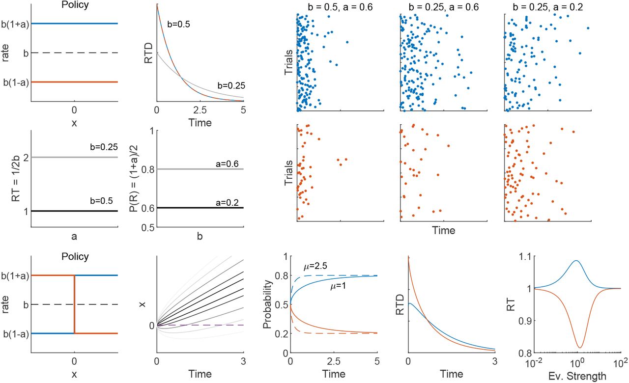