Optimal clustering for quantum refinement of biomolecular structures: Q|R#4

Abstract

Quantum refinement (Q|R) of crystallographic or cryo-EM derived structures of biomolecules within the Q|R project aims at using ab initio computations instead of library-based chemical restraints. An atomic model refinement requires the calculation of the gradient of the objective function. While it is not a computational bottleneck in classic refinement it is a roadblock if the objective function requires ab initio calculations. A solution to this problem adopted in Q|R is to divide the molecular system into manageable parts and do computations for these parts rather than using the whole macromolecule. This work focuses on the validation and optimization of the automatic divide-and-conquer procedure developed within the Q|R project. Also, we propose an atomic gradient error score that can be easily examined with common molecular visualization programs. While the tool is designed to work within the Q|R setting the error score can be adapted to similar fragmentation methods. The gradient testing tool presented here allows a priori determination of the computationally efficient strategy given available resources for the potentially time-expensive refinement process. The procedure is illustrated using a peptide and small protein models considering different quantum mechanical (QM) methodologies from Hartree-Fock, including basis set and dispersion corrections, to the modern semi-empirical method from the GFN-xTB family. The results obtained provide some general recommendations for the reliable and effective quantum refinement of larger peptides and proteins.

1. Introduction

Accurate and reliable structures of bio-macromolecules at an atomistic level have been instrumental in our understanding of biological processes [1, 2, 3], drug design [4] or protein engineering [5]. Atomic model refinement provides an efficient route to obtain high-quality models of such molecules. Refinement takes an atomic model and improves it to optimally match the data that originates from a crystallographic or cryo-EM experiment [6]. However, the limited resolution of the experimental data and low data-to-parameter ratio require the refinement procedure uses a priori chemical information. This chemical information is utilized as stereo-chemical restraints or constraints [7, 8] (such as bond lengths, bond angles, torsion angles, and so on) and originates from various sources, such as small molecule databases (Cambridge Structural Database (CSD) [9, 10], Crystallography Open Database (COD) [11]) or the ultrahigh-resolution protein structures (Conformation Dependent Library (CDL) [12, 13, 14]). These restraints are limited to the information available in the databases and fail to easily cope with novel chemical moieties such as new drugs [15, 16, 17, 18] or unusual local arrangements [19, 20, 21]. Also, they do not account for electrostatic effects [19] or local and typically unique to the structure non-covalent interactions such as hydrogen bonds, salt bridges, π-stacking and more [22, 23].

Quantum mechanical (QM) methods have proven to be powerful, predictive tools in protein structure research [24, 25, 26, 27, 28, 29]. One of the examples is our newly developed quantum-based refinement (Q|R) package [30] that combines QM and crystallographic [26] or cryo-EM [27] experimental data. The Q|R software is developed as an open-source module of the Phenix package [31]. It does not require any of the static library-based parameterized restraints (such as Monomer Library; [32, 33]) using QM calculations instead. The existing developments that use quantum mechanical calculations as a source of restraints for macromolecular crystallographic refinement employ methods based on multiscale QM/molecular mechanics (MM) [34, 35], semi-empirical [3] or linear-scaling density functional theory [36]. These tools typically focus on the region of particular interest in the macro-molecule (e.g., ligand or ligand-binding pocket) while neglecting the rest of the model or treat it with the standard classic approach using stereo-chemical restraints. In Q|R based refinements the whole protein structure is treated at the QM or semi-empirical (SQM) level, for example, the HF/6-31G level, employing also London dispersion (D3) [37] and basis set incompleteness (gCP) corrections [38] or by GFN-xTB [39], accounting for the polar environment by means of continuum solvent model (CPCM/COSMO [40] or internal xtb generalized born (GB) solvation model).

QM restraints provide more chemically meaningful bio-macromolecular structures [41]. However, the issue of computational scalability in QM methods [42] is one of the main obstacles to perform reliable and efficient QM calculations in the quantum-based refinement. Although computational algorithms and hardware resources steadily improve, this issue remains [43].

The atomic model refinement requires calculation of an objective function value and its gradients with respect to refinable parameters (e.g., Cartesian coordinates), where the objective function is a weighted sum of stereochemical restraints (classic or quantum) and the experimental data term [6]. To address the scalability issue the whole QM gradient can be computed by one of the divide-and-conquer methods [29, 44, 45, 46, 47]. Assuming that the molecules in the local area of the macro-molecular system are hardly affected by the molecules further away, in principle, any large protein can be divided into a group of smaller pieces [44, 48]. In the Q|R project we are using our own partitioning scheme [49] where the macromolecule is divided into clusters. A fragment contains the cluster and its surrounding buffer region. This partitioning algorithm is crystallographic symmetry-aware [50]. Since the energies arising from individual clusters cannot be combined into the total energy, the Q|R refinement only uses the energy gradients. The QM energy gradients for all atoms from each of the fragments are computed with only the gradients from each cluster combined to create the total gradient. This procedure has been already successfully applied to improve several molecular models by quantum refinement in connection with experimental data from X-ray crystallography [49, 50] and cryo-EM [51]. It has been also used in the QM optimization of protein structure [51]. The divide-and-conquer procedure can potentially introduce and accumulate errors at the dividing boundaries of the clusters due to, for example, insufficient size of the buffer region. This problem can be readily alleviated by expanding the buffer region which in turn will increase the time of computations (often by a large margin).

Here we continue our series [30, 49, 50, 51] of publications that document the evolution and progress of the Q|R project. In what follows we describe how divide-and-conquer procedure can be optimized to minimize these errors without substantial increase of the computational time, which sets another milestone along the road of the Q|R project.

2. Methods

2. Model selection and preparation

We use two of the models from the test set of 70 peptide and protein structures employed in previous works [52]. The first model (PDB entry 3ftL, 17 residues, 109 atoms, 1.60 Å resolution) is sufficiently small to allow the detailed analysis of all possible clustering schemes as well as an extensive testing of parameters defining fragments for which QM computations are performed. 3ftL is an amyloid peptide with highly ordered and packed aggregates stabilized by intermolecular contacts spanning across symmetry copies [53]. This makes this model a suitable candidate for a validation and analysis of Q|R divide-and-conquer procedure. The second model (PDB entry 3q2c, 128 residues, 787 atoms, 2.50 Å resolution) has been selected as a larger and more complex example with different secondary-structure patterns. These models were prepared for test as following. The atomic model and reflection data files have been obtained from the RCSB PDB Database [54] and then refined using phenix.refine [31, 55] using default settings in order to obtain an optimal starting point. The model was next completed by adding hydrogen atoms using the qr.finalise [30] tool that is part of the Q|R software suite. The resulting models (3ftL 209 atoms, 3q2c 1611 atoms) have been used for the gradient analysis using Q|R. Additionally, the similar tests have been performed for the models used previously [51].

The crystallographic symmetry-aware divide-and-conquer procedure in Q|R [49, 50] includes expansion of the unit cell content in space, which is referred to as super-sphere. The super-sphere contains the model in question and residues from symmetry copies that fall within a pre-defined distance (R_SS) from the model. This symmetry expansion distance (R_SS) is set to 10 Å by default. Once the super-sphere is obtained, the model is partitioned into fragments, where each fragment is composed of one cluster and surrounding buffer region. The buffer region is needed to account for covalent and non-covalent interactions and should be sufficiently large for accurate QM calculations. If needed, the buffer region can be further extended to create a so-called double-buffer by adding another layer of residues, interacting with a previously constructed (single-buffer) fragment. It should be noted that the R_SS distance does not affect division of model into clusters, but only influences the size of buffer region.

2.2 Automated testing for accuracy of QM gradient

Clustered gradient is the gradient for the whole model that is calculated as an accumulation of individual gradients arising from each cluster. Therefore, the clustered gradient is an approximation to the exact gradient calculated for the whole model. This is because surrounding atoms interact with the cluster through covalent and non-covalent interactions. Inaccuracies of the clustered gradient arise from the two aspects of making a cluster: cutting through covalent bonds (followed by capping of naked atoms at the cut) and limiting the non-covalent interactions. Calculation of the clustered gradient (and therefore its accuracy) is governed by several parameters, such as (i) R_SS distance used to define the super-sphere, (ii) maximum allowed number of residues in each cluster, (iii) size of the buffer region surrounding each cluster (e.g., single- or double-buffer). The larger the super-sphere and the thicker the buffer, the more accurate clustered gradient will be and the more time will be required to calculate it. However, the gradient from the whole model and the clustered gradient can never match exactly due to numerical errors and errors arising from capping. An automated procedure described here aims at obtaining the set of these parameters that minimize the errors in the clustered gradient using the least computational time possible. For this a new command-line tool was added to the Q|R project named qr.gtest. To evaluate the error in the clustered gradient a reference to compare with (e.g., the exact gradient) is needed. This reference gradient is calculated only once either from the whole super-sphere (if computationally possible) or from the clustered gradient obtained with the sufficiently large buffer region (if the molecule is too large to use the whole super-sphere). In this work we use the gradient calculated from the super-sphere as the reference.

There are two options available in the qr.gtest. One will proceed with the computation of the reference gradient where the model is not divided at all. In that case the QM gradient is computed for the whole super-sphere. The second option tests (i) different possibilities of the maximum allowed number of residues in each cluster, which define how the model is divided; and (ii) the size of the buffer region needed for each cluster. In all cases qr.finalise is used to cap atoms to assure correct atomic valences at cutting points.

In this work we have tested the effect of the super-sphere size on the gradient error by considering the R_SS distance between 1 and 30 Å for the computations of QM gradients. Additionally, we analyzed the fragment size and composition obtained with single- and double-buffer.

2.3 Analysis and error evaluation for the clustered gradient

In order to analyze errors in clustered gradient the computation of reference gradient and the gradient obtained from divide-and-conquer procedure (clustered gradient) with different set of parameters are required. Then QM gradients computed for all clusters are analyzed with respect to the reference. Technically this is done by the qr.granalyse (“gradient analyse”) tool that automatically collects previously calculated and stored gradients and sorts them according to fragment and buffer size, and takes the gradient with the largest buffer (or if available from super-sphere) as reference unless manually specified otherwise. For each gradient an analysis described in the following is done and a PDB file is written for visualization. For each atom i in the model a measure of the atomic-gradient error (here referred to as the weighted difference gradient δ_i) is computed and written into the B-factor field of the PDB file. That allows an easy color-shaded visualization of δ_i using standard biomolecular viewers.

In the error statistic we follow the idea of a regularized error [56], where we consider relative errors for large gradient differences and absolute errors for the small ones with the goal to bring both at a comparable level. As the regularisation we have chosen to use the median over all atomic gradients, instead of an arbitrarily pre-defined value as in [56], because the magnitude of the energy gradients is generally unknown. This choice was tested by detailed inspection of all gradients and their errors for the 3ftL case confirming that this metric follows what could be intuitively considered as small and large errors.

Firstly, we define the nuclear gradient matrix as with N being the number of atoms. For each atom i the atomic difference gradient ΔG_i is expressed as the sum of the differences of the 3 cartesian component (c=x, y, z) with respect to the reference: Finally, the weighted difference gradient δ_i for atom i is computed as and the average over all N atoms is Where ||ΔG_i|| is the norm of the difference gradient for the atom i, ||g_ref(i)|| the norm of the reference gradient for the atom i and Median (||g_ref(N)||) the median of all the reference gradient norms. Considering the reference gradient norm allows treating the magnitude of errors for small and large gradients on a more equal footing, while regularization with the Median gradient prevents too small gradients in the denominator from skewing the analysis. Moreover, for all cases where δ_i is larger than 100 (possible for example if the reference and tested gradients are of opposite sign) the final value is set to 100 to mimic the percentage and treat different cases on a comparable scale. Here we use a colour scheme with dark blue being 0 and 100 being red (in PyMol the command is “spectrum b, minimum=0, maximum=100”).

2.4 QM computations

The Q|R uses the ASE package [57] to interface with many modern QM computational software that can be used to calculate the gradients. In this work, we use TeraChem [42, 58, 59] and xtb [39] as QM calculators. TeraChem is a program employing Graphics Processing Units (GPUs) as a computing architecture for electronic structure calculations, which in turn allows efficient QM computations for thousands of atoms [58]. TeraChem calculations were performed with the Hartree-Fock (HF) method and the 6-31G basis set, with Grimme’s dispersion correction D3 [37] and the appropriate corrections for the basis set incompleteness via geometrical counterpoise model (gCP) [38]. The gCP and D3 corrections are implemented as part of qr.refine add-ons using standalone gcp [38] and dftd3 [37] programs. Moreover, the environmental effects have been described employing the COSMO polarizable continuum solvent model [60]. The TeraChem computations have been performed on a Tesla K80 graphical card using 4 GPUs for the single QM run. The available computational resources consisted of total 48 cores, so that 12 single gradient computations can run at the same time.

The xtb computations were performed with the first-generation method named GFN1-xTB with bulk solvent effects treated using the internal generalized born (GB) solvation model. The GFN1-xTB calculations were executed on an Intel(R) Xeon(R) CPU E5-2690 v4 @ 2.10GHz CPU with a total of 28 cores or an Intel Core i9-10900X CPU with 3.7 GHz frequency and 20 cores.

3. Results

3.1 Sensitivity of the clustered gradient to the super-sphere size and QM methods

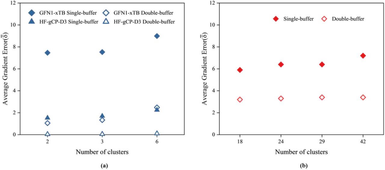
We start by comparing gradients computed for the whole model, without any clustering, but with increased surroundings, which is defined by the super-sphere R_ss. We use gradients calculated with the largest super-sphere as the reference. The 3ftL peptide unit cell has only 209 atoms, but due to the close packing the number of atoms in the super-sphere increases rapidly with the Rss distance, at some point reaching as many atoms as in a relatively large model (such as 3q2c with 1611 atoms), as illustrated in Fig. 1a. The super-sphere obtained with the R_ss of 15 Å (7321 atoms for 3ftL and 8288 for 3q2c) is the largest for which the less expensive GFN1-xTB computations can be performed with our computer resources, which was considered as the reference. The trial gradients were computed with the R_ss sampled between 1 and 14 Å. Fig. 1b shows the average gradient error . Starting from about 7 Å, the gradient errors become small and reach the plateau. Fig. 2 shows per-atom δ_i values for the 3ftL model calculated using four different Rss values. Clearly the choice of R_ss being 7 Å yields accurate gradients for all atoms (Fig. 2d). The R_ss of 7 Å is also largest for which more expensive HF-gCP-D3 computations can be performed. Fig. 1c shows that obtained at HF-gCP-D3 level are smaller than GFN1-xTB, albeit at a higher computational cost. Considering that the default radius of 10 Å would cause unnecessary computational effort due to significantly larger number of atoms (3220) the R_ss of 7 Å (1951 atoms) was used in subsequent analyses for 3ftL in conjunction with all QM methods. At variance, for 3q2c only GFN1-xTB method was considered so the default R_ss of 10 Å has been used as computationally feasible.

Fig. 1.

Super-sphere at different Rss (a) Number of atoms for 3ftL and 3q2c (the Rss range up to 12 Å is zoomed in the inset). Average atomic gradient error with respect to super-sphere Rss of (b) 15 Å for 3ftL and 3q2c computed at the GFN1-xTB level and (c) 7 Å for 3ftL computed at the HF-D3-gCP and GFN1-xTB levels.

Fig. 2.

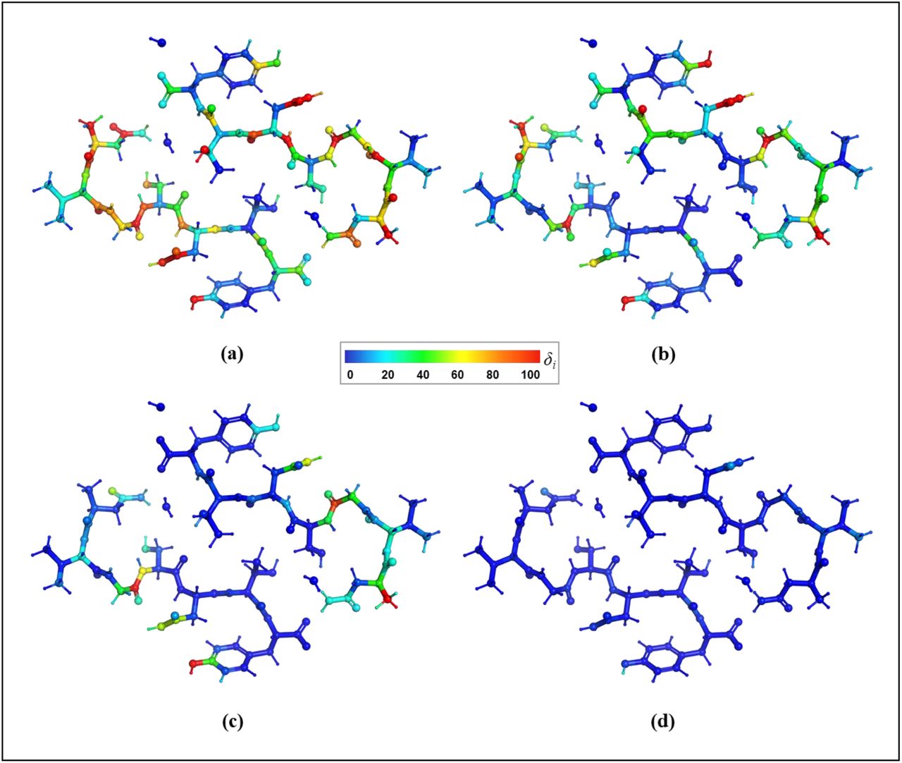
3ftL model colored by the atomic gradient errors for super-sphere with different R_ss (1 Å, 3 Å, 5 Å, 7 Å): (a, b, c, d) with respect to the reference with R_ss=15 Å computed at the GFN1-xTB level.

3.2 Sensitivity of the clustered gradients to clustering

Here we analyze how the size and number of clusters affect the clustered gradient error. The 3ftL model can be partitioned into clusters using Q|R’s divide-and-conquer method in three different ways yielding 6, 3 and 2 clusters as shown in Fig. 3. For larger 3q2c protein there are more possibilities, so only some have been considered in this analysis. Fig. 4 shows average gradient error with respect to the clustering choice, in conjunction with smaller or larger buffer region. We observe that for given QM method and buffering the errors are very similar for all clustering choices.

Fig. 3.

Three possible partitioning (clustering) of the 3ftL model

Fig. 4.

Average atomic gradient error for different clustering and buffers (a) for 3ftL computed at the HF-gCP-D3 and GFN1-xTB levels. (b) for 3q2c computed at the GFN1-xTB level.

3.3 Sensitivity of the clustered gradients to buffer size

Here we study how the size of the buffer affects the accuracy of the clustered gradient. Clearly, the larger is the buffer the smaller are the errors in the clustered gradient (Fig. 4). For example, in case of 3ftL the largest errors resulting from using double versus single-buffer are an order of magnitude smaller (1-2 versus 25). However, the larger the buffer the longer it takes to calculate those gradients. Therefore, an optimal choice of the buffer is important. For that reason we analyse in more detail the atomic gradients obtained with different buffers in order to rationalize situations leading to significant local errors. Highlighted cases include examples of local errors arising from cutting through covalent and non-covalent interactions within the model as well as due to expansion by the crystallographic symmetry.

3.3.1 Covalent bonding within unit cell

The 3ftL peptide is composed of two symmetrical loops, each loop consisting of seven residues. In all clustering procedures, each of the A and B chains is cut at the N atom on Threonine (residue number 6), so the gradient error on these atoms has been analyzed in more detail.

When cutting the model into two clusters (Fig. 3), this N atom in chain B shows a negligible gradient error of 1.3 (Fig. 5a) but this error is 18.2 in the same atom in chain A (Fig. 5b). This can be explained by differences in the buffer region. In case of single-buffer, for the chain A only one residue is added after the cutting point (Fig. 5b), while for the chain B there are two residues past the cut (Fig. 5a). In the case of double-buffer both chains have at least three additional residues after the cutting point (Fig. 5c, d), which reduces the error from 18.2 and 1.3 (single-buffer) to 0.2 and 0.1.

Fig. 5.

The 3ftL model divided into two clusters, showing fragments including single-buffer (a, b) and double-buffer (c, d). The clusters (colored by atomic δ_i values as computed at HF-gCP-D3 level) include two border-line nitrogen atoms. All atoms from buffer region are shown in grey, among them the residues directly behind the N atom in the chain are highlighted (grey ball and stick). The δ_i on both nitrogen atoms are reported in insets.

3.3.2 Non-covalent interaction within unit cell

For the 3q2c the largest gradient errors appear on the oxygen and carbon atoms of the Valine residue 22 in chain A, with δ_i of 92.8 and 56.0, respectively (see Fig. 6a). This oxygen atom is involved into the hydrogen bond O···H-N with the Isoleucine 62 in chain A from the buffer region. In turn, this Isoleucine residue is truncated in the single-buffer and capped with a hydrogen atom. Using the double-buffer adds residues prior and past Isoleucine 62 (Fig. 6b), creating a six-residues chain and reducing the gradient error down to 0.8 and 3.3 on O and C, correspondingly.

Fig. 6.

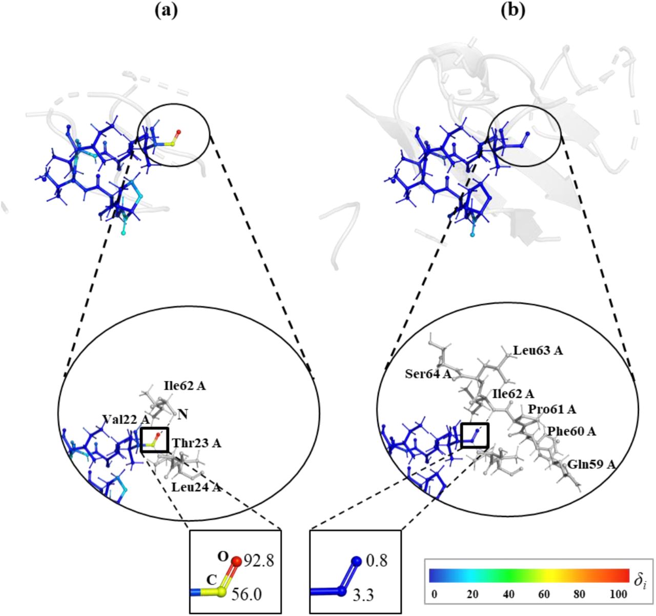
The 3q2c model, with non-covalent bonding inside unit cell, showing the δ_i on C and O atoms of residue Val 22 in chain A using (a) single- and (b) double-buffer.

3.3.3 Interactions with symmetry copies

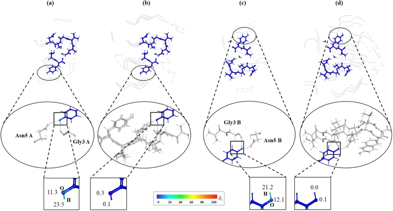
For the 3ftL model the largest errors in the clustered gradient were observed for H atoms involved in hydrogen bonding with symmetry copies. Namely, the hydrogen bonds D-H···A where either the hydrogen donor (D) or acceptor (A) belong to buffer region.

An example is the hydroxy groups in Tyrosine residue 7 in both chains that interact with symmetry copies (Fig. 7). Using the single-buffer results in errors around 11 and 23 on OH and HH in both chains, correspondingly, even though the directly interacting residues (Glycine 3 -- proton acceptor and Asparagine 5 -- proton donor) are present. Using the double-buffer includes more surroundings and that reduces these errors down to almost zero.

Fig. 7.

The interaction with symmetry copies for 3ftL model around H atom of TYR7. Different buffer environments for two clusters case (chain A a, b and chain B c, d): single-buffer (a, c) and double-buffer (b, d). All atoms in clusters are coloured by atomic δ_i values while the residues from buffer region are shown in grey.The enlarged circle in the middle highlights the hydrogen bonds formed with the atoms from the buffer. The boxes at the bottom zoom on O and H atoms from TYR7 and report their weighted difference gradient δ_i values.

Fig. 8.

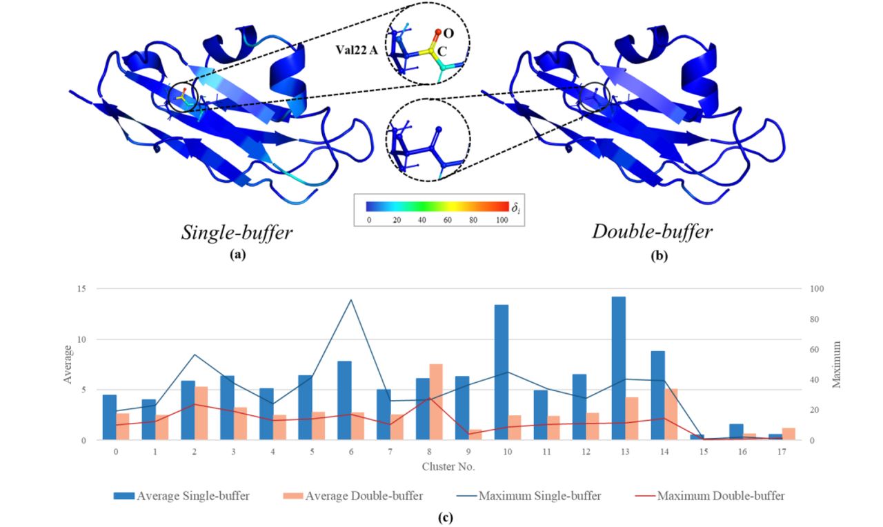
Atomic gradient errors for 3q2c protein: atomic δ_i in single- (a) and double-(b) buffer environments; average and maximum δ_i for each cluster (c).

3.4 Accuracy of clustered gradient for larger proteins

The gradient error analysis has been also performed for protein models with up to 7000 atoms (PDB codes: 3j63, 3a5x and chain C of 5fn5) that have shown significantly improved geometry metrics after quantum refinement in our recent study [51]. All gradients have been computed with the GFN1-xTB model and single-buffer, as employed in the Q|R #3 paper [51]. For the 3j63 and 5fn5 both super-sphere and double-buffer have been considered as reference, and only latter for the largest 3a5x. In all cases minimal gradient errors have been achieved with average and maximum δ_i below 1 and 10, respectively.

3.5 Timings

Among reliable divide-and-conquer schemes the choice of preferred one for computationally extensive refinement can be done based on the time required to compute single complete gradient. For that there are two limiting factors: (i) the size of the largest fragment which defines the most time consuming QM computation; (ii) the total number of atoms in all fragments which defines the total CPU or GPU time needed to compute all gradients. We note that gradients for all fragments need to be computed in order to construct total clustered gradient. So, if all QM computations can run in parallel the size of largest fragment is the bottleneck factor, and division to larger number of smaller clusters is preferred. Second possibility is that all computations are run in serial. In that case division to smaller number of larger clusters, with smaller can be preferred.

However, in practice most common can be the third situation, that is number of clusters being larger than number of jobs which can be run in parallel. In this latter case, it might be cumbersome to decide ad hoc an optimal computational set-up, due to vast possibility of tunable parameters (clustering scheme as well as how many jobs (J) shall be run in parallel on how many cores (C) given the total number (M) of the latter (either CPU or GPU, M=J x C). These three situations are illustrated for 3ftL and 3q2c in Table 1 showing the timings required to compute a single gradient using HF-gCP-D3 (TeraChem) or GFN1-xTB (xtb).

Table 1.

Number of atoms in clusters and fragments for 3ftL and 3q2c from different clustering choices along with the time needed to compute single complete gradient from TeraChem (HF-gCP-D3) or xtb (GFN1-xTB).

For 3ftL the cluster size ranges from 3 (a single water molecule) to 106 atoms (one complete chain), with fragment sizes varying from 127 to 787 atoms for a single-buffer and 532 to 1678 atoms for a double-buffer. This clearly indicates a notably higher computational cost for the latter. First situation is indicated by TeraChem computations, i.e. our GPU resources allowed computing gradients for all fragments at once using HF-D3-gCP, so in practice the total timing was determined by . In the present case six clusters with the smallest possible fragments was the most effective scenario for both single- and double-buffer. Second situation is illustrated by GFN1-xTB computations (set to run sequentially) where two/three clusters is more favorable because the total number of atoms is reduced by about 30% compared to six clusters.

For 3q2c we consider only four possible clustering scenarios with the smallest number of clusters being 18. These computations were executed on the architecture with 20 cores, and we arbitrarily chosen to run 4 single gradient computations each one performed using 5 CPUs. This mimics the third situation: number of separate gradient calculations which run at a time is smaller than the total number of clusters. Therefore, computations are performed both in parallel and sequentially, which for this test-case leads to optimal situation with 18 clusters for both single- and double-buffer.

In more general terms the gtest procedure allows testing of realistic timings to find the most optimal for the specific model and computer resources. As during the course of a refinement many gradients will need to be calculated, the effort put into testing the timing of different clustering approaches will pay off in the long run.

3.5. Optimize time and gradient error

Increasing the buffer region clearly leads to improved atomic gradients. For 3q2c significantly lower δ_i are obtained for the double-buffer, with the all-atoms average and maximum of 3.2 and 28.1, respectively. For the single-buffer environment most of the atomic gradients also show small errors, but outliers with δ_i over 30 are present in half of the clusters, and over 50 in two clusters, leading to the δ_i averaged over all atoms equal to 5.9.

This shows that the extension of the buffer region for specific clusters represents a promising and cost-effective strategy to deal with well-localized outliers, avoiding an unnecessary buffer extension in well-behaved parts. Automatic gradient errors analysis allows implementing an adaptive “mixed” buffer strategy, into the qr.refine. The procedure starts from the computation of atomic δ_i, which indicate if there are any clusters for which single-buffer environment is not sufficient. If that is the case, the buffer region is extended only for the specific clusters. This way the total number of atoms for which QM computations are required is reduced compared to the double-buffering applied to the whole model, saving computational resources. The number of atoms in all fragments obtained with different buffering strategies, relevant timings and maximum and average δ_i are reported for 3q2c in the Table 2. Considering a conservative maximum δ_i of 30 as the threshold, the total number of atoms in all fragments doubles with respect to single-buffer, but is still 30% smaller than for the full double-buffer. For the δ_i threshold of 50 there is an increase of atoms by 40% with respect to single, and decrease by 50% with respect to double-buffer, respectively. Corresponding computational time increases with respect to single-buffer by 5 to 2.5 times for Max>30 and Max>50 respectively, but is still about halved compared to double-buffer, without introducing outliers. As more experience is gained with other systems, the threshold can be fine-tuned in the future.

Table 2.

The number of atoms in fragments from different divide-and-conquer schemes for 3q2c along with the time needed to compute single complete gradient from GFN1-xTB restraints.

Another possibility for reducing gradient errors is extending buffer for specific cluster by expanding single-buffer with the smallest possible number of residues. Fig. 9 shows δ_i on atoms involved in hydrogen bonds with buffer region, where 3q2c Val22 acts as a proton donor (N-H···O) or acceptor (C=O···H-N). The latter correspond to the largest gradient errors for single-buffer as discussed in section 3.2.2. By adding into buffer just one residue (Pro61) large errors on oxygen and carbon atoms are reduced from δ_i of 92.8 and 56.0, respectively to about 25 on both atoms (Fig. 9a). However, at the same time errors on nitrogen and hydrogen from adjacent hydrogen bond increase with respect to single-buffer case, from 8.5 and 12.2 to 29.7 and 61.7, respectively. So, another unbalanced environment is created. The latter problem is resolved by adding one residue after Ile62 (Fig. 9b), which reduces errors below 20 on all N, H, C and O of Val22. Overall, a balanced description requires symmetric buffering – one (Fig. 9b), or two (Fig. 9d) residues added on both sides of Ile62, while asymmetric situations (Fig. 9a, c) show larger errors. This analysis indicates that definition of reduced, yet smaller buffer region might be a non-trivial task.

Fig. 9.

The 3q2c model, δ_i on C, O, N and H atoms of residue Val 22 in chain A for buffer cases between single- and double-buffer (reported in Fig. 6a and 6b, respectively). Possibilities consider adding one-by-one residues to the amino acid backbone in the fragment.

Conclusions

Herein we analyze the robustness of the QM nuclear gradient from the divide-and-conquer procedure employed during quantum refinement in the Q|R project. Moreover, we present new parts of the Q|R code called gtest and granalyze that help to automate assessment of the gradient quality.

The procedure was showcased for the 3ftL peptide and 3q2c protein where errors in energy gradients were analysed with respect to super-sphere size, clusters of different sizes and increasing buffer regions, by comparing to a reference gradient obtained from a super-sphere calculation with large R_ss. We introduced an error metric that allows to pin-point errors in the gradient to specific atoms or groups that then can be checked for missing interaction with, e.g. symmetry-copies or near-by residues, due to an insufficient buffer region. To simplify the analysis for the user the tool writes PDBs files with color coding to allow an intuitive visual inspection.

Different QM methods show a similar sensitivity to the clustering parameters, with overall gradient errors for using HF-gCP-D3/6-31G, being smaller than for the semi-empirical quantum methods GFN1-xTB.

Moreover, we showed that by applying the double-buffer procedure essentially error-free gradients can be obtained for the case when the super-sphere calculation is computationally prohibitive.

The presented granalyze procedure is an effective tool by which diverse divide-and-conquer schemes, varying by number of residues in the cluster or the applied buffer region can be easily tested, the most computationally efficient setup chosen and their errors analyzed. This allows also implementing new strategies for the efficient choice of adaptive buffer region during quantum refinement, avoiding unnecessary environment expansion for the parts of molecular model with already error-free gradient. Finally, both automatic partitioning scheme and gradient analysis tools from Q|R can be employed to define divide-and-conquer strategies for other QM computations of bio-macromolecules, beyond the quantum refinement.

All the tools developed within the Q|R project are available at https://github.com/qrefine/qrefine.

Gradient error analysis results and related data are available at: https://github.com/qrefine/QR4-Gtest.

Author Contributions Statement

MB, HK and PVA wrote the main manuscript text. HK developed tools describe in the manuscript. YW performed all computations, analysis and prepared figures. PVA, NWM, MPW and HK developed the overall code. All authors reviewed the manuscript.

Acknowledgments

MB and YW acknowledge the financial support from the National Natural Science Foundation of China (Grant No. 31870738). MB also acknowledges support of the COST Action CA21101 “COSY”.

Footnotes

• https://github.com/qrefine/QR4-Gtest