

Abstract
Important traits in agricultural, natural, and human populations are increasingly being shown to be under the control of many genes that individually contribute only a small proportion of genetic variation. However, the majority of modern tools in quantitative and population genetics, including genome wide association studies and selection mapping protocols, are designed to target the identification of individual genes with large effects. We have developed an approach to identify traits that have been under selection and are controlled by large numbers of loci. In contrast to existing methods, our technique utilizes additive effects estimates from all available markers, and relates these estimates to allele frequency change over time. Using this information, we generate a composite statistic, denoted Ĝ, which can be used to test for significant evidence of selection on a trait. Our test requires genotypic data from multiple time points but only a single time point with phenotypic information. Simulations demonstrate that Ĝ is powerful for identifying selection, particularly in situations where the trait being tested is controlled by many genes, which is precisely the scenario where classical approaches for selection mapping are least powerful. We apply this test to breeding populations of maize and chickens, where we demonstrate the successful identification of selection on traits that are documented to have been under selection.
Introduction
Quantitative traits encompass an inexhaustible number of phenotypes that vary in populations, from characters such as height (Yang et al. 2010) to weight (Barsh et al. 2000) to disease resistance (Poland et al. 2009). These types of traits are so essential for agriculture and human health that the entire field of quantitative genetics revolves around their study (Plomin et al. 2009; Wallace et al. 2014). However, the nature of quantitative traits makes it difficult to study their genetic basis; for nearly a century, scientists have modeled quantitative traits by assuming that their underlying control involves many loci each contributing a very small proportion to genetic variance (Fisher 1918), the so-called ‘infinitesimal model’. Therefore, conducting studies with enough power to identify a substantial proportion of the loci that contribute to a quantitative trait requires a massive sample size, imposing financial and logistical barriers. However, this model of quantitative trait variation does an excellent job when predicting important characteristics such as response to selection (Visscher et al. 2008). For instance, the recent development of genomic prediction methodologies (Meuwissen et al. 2001) allow the breeding value and/or phenotype of individuals to be predicted with remarkable precision from genomic information alone.
The models of quantitative genetics have had a less dramatic impact on studies of evolutionary adaptation, where genomes are often scanned to identify adaptive loci with large effects (Akey 2009). Positive selection on such loci leaves behind pronounced signatures, deemed “selective sweeps”. There is an abundance of evidence for such sweeps in humans (Sabeti et al. 2007), natural populations (Schweizer et al. 2016), livestock (Qanbari and Simianer 2014), and crops (Hufford et al. 2012; Qanbari and Simianer 2014; Schweizer et al. 2016). However, alternative forms of selection, including purifying selection against new mutations (Lawrie et al. 2013), selection on standing variation (Garud et al. 2015), or selection on many loci of small effect (Turchin et al. 2012), rarely leave these discernible signatures at individual loci. Evidence of these forms of selection can be difficult to identify. When they can be found, it is often through the pooling of weak evidence at individual loci into a stronger signal across a class of loci. For example, Beissinger et al (2016) demonstrated the importance of purifying selection during maize evolution by combining evidence from all maize genes. An approach implemented by Berg and Coop (2014) tests for evidence of selection on a quantitative trait by evaluating allele frequencies at all loci that have previously been implicated by genome-wide association studies (GWAS) as putatively associated with that trait. This approach has since been used to test for selection on multiple human traits, including height (Mathieson et al. 2015) and telomere length (Hansen et al. 2016).
In studies of model organisms or agricultural species, large collections of previously identified “GWAS hits” are not as abundant as in humans, on which the Berg and Coop (2014) method depends. This is due in part to the more modest sample sizes that tend to be used in experimental settings compared to clinical studies, often combined in large-scale meta-analyses (Evangelou and Ioannidis 2013). In contrast to humans, however, genotypic data across multi-generational time points are often available for model and agricultural species. We have developed a test for selection on complex traits that leverages such genotype-over-time data. Our test depends on the relationship between the change in allele frequency across generations and the estimated additive effect of the same allele, computed for every genotyped locus. We use these values to compute an estimate of the direction of genetic gain, which can be shown to be additive across all loci considered and lends itself to a straight-forward positional dissection of the accumulated genetic gain. Because phenotypic data are incorporated, a permutation-based test for significance can be utilized so that significance testing is not limited by many of the demographic history and population structure related caveats that complicate determining significance when testing for selection (de Villemereuil et al. 2014). Our method utilizes additive effects estimates for each locus calculated simultaneously, using shrinkage-based methods that have been honed over the past 15 years for the purpose of genomic selection and prediction (Campos et al. 2013). Therefore, this text can be considered analogous to reverse genomic selection; rather than using predictions of breeding value to drive selection and hence future changes in allele frequency, we use the same data coupled with knowledge of past changes in allele frequency to make inferences regarding which traits were effectively under selection in the past. Interestingly, we find by simulation that this approach is most powerful for identifying selection on traits controlled by many loci of small effect, which is exactly the situation where other tests for selection and/or association are least powerful.
Herein, we first describe our test for selection on complex traits. Then, we perform simulations demonstrating the validity of the method and explore the situations where it is most and least powerful. Finally, we apply the method to breeding populations of maize and chicken. In both of these experimental situations, we successfully identify the traits that are known to have been selected. Collectively, our results demonstrate that this approach may be leveraged to identify novel traits or component-traits that may be used to inform future breeding decisions and/or for enhanced historical, ecological, and basic scientific understanding.
Results
Theoretical Motivation
Assume that a trait is fully controlled by additive di-allelic loci j = 1, … m. Then the genotypic value, aj, of an allele at locus j, is equal to its gene substitution effect, αj. Based on this equivalency, the mean phenotypic effect, Mj, attributable to the locus is given by Mj = αj(2pj−1), where pj, is the frequency of the reference allele at this locus. It follows that the change in the population mean resulting from selection on this locus, what we may consider the locus-specific response to selection, is given by
 where pj0 is the allele frequency before selection and pj1 is the allele frequency after selection. Define Δj = (pj1-pj0), leading to Rj = 2 Δjαj. Based on our earlier assumption of complete additivity, summing over all m loci provides a genome-wide estimate of the response to selection (Falconer and Mackay 1996):

This estimate of selection response also naturally arises from the logic of random regression BLUP (RRBLUP) (Meuwissen et al. 2001). Here, a model is used
 where y is a vector of length n containing phenotypes for a specific trait, b are fixed effects,
  is the vector of length m containing additive SNP effects at m loci;
  is the vector of random residual terms, and
  and
and  are the corresponding variance components. X and Z are incidence matrices linking observations in γ to the respective levels of fixed effects in b and random SNP effects in s. In more detail, Z is an n × m matrix where element Zij contains the genotype of individual i at SNP locus j. Since such models are invariant with respect to linear transformations of the allele coding (Strandén et al. 2011), we may use the notation
  , or 1, standing for zero, one, or two copies of the reference allele. Note that with this coding, sj is equivalent to 2αj in the coding above, since it reflects the contrast between the two homozygous genotypes at locus j. Due to the equivalence of genomic BLUP (GBLUP; VanRaden 2008) and RRBLUP (Endelman 2011), it is possible to calculate genomic breeding values of the genotyped individual as û = Zŝ, where ŝ are the solutions for the SNP effects obtained using RRBLUP with model (2).
Assume now further that individuals in the vector y can be assigned to g discrete generations and that the individuals of the oldest generation come first and the individuals of the last generation come latest. We then can define a g × n matrix
 where li is a row vector of length ni, which is the number of individuals in generation i, of which all elements are 1 /ni. With this, a vector ū of length g reflecting average breeding values per generation can be calculated as ū=Lû, and estimated selection response results as
  .
.
Now, ū =Lû = LZŝ, where LZ is a g × m matrix in which element í, j reflects the average allele frequency of the reference allele at SNP j in generation í. The allele frequency change between generation 1 and generation g can be obtained as a linear contrast between the first and the last row of this matrix as Δ=k’LZ where k is a vector of length g with k1 = −1, kg = 1, and all other elements are zero. Finally, the selection response can be written as R = Δŝ, which is identical to equation (1), given that s is equivalent to 2α.
Furthermore, theory suggests that under the assumption that selection intensity is equal for all genes across the genome, the change of allele frequency Δi should be approximately proportional to the allele effect αi, such that for a trait under selection a non-zero correlation between allele frequency change and the additive effect of alleles on that trait is expected (Wright 1937). Alternatively stated, (1) emphasizes the temporal component of the Breeder’s Equation, R = h2S, where h2 is the narrow-sense heritability of a trait and S is the selection differential. Given a population of individuals with more than one time-point of genotypic data, it is simple to compute Δi for every genotyped locus. Furthermore, the shrinkage methods of genomic prediction (Campos et al. 2013), including Ridge Regression (Endelman 2011) and GBLUP (VanRaden 2008) allow additive effects, αi, to be approximated for every genotyped position. For this, a set of individuals genotyped and phenotyped in at least one generation is needed.
A notable benefit of the estimator in (1) is that by leveraging temporal data from genotypes rather than from phenotypes, it only requires one generation of phenotyping. Additionally, this suggests that if we consider R a random variable, then given the distribution of R in a scenario without selection, a test of whether or not Ȓ is different from zero may be performed. Since Ȓ is the genomic response to selection, this is equivalent to testing whether or not a trait has been under selection during the timeframe under study.
Significance Testing
We implemented a permutation-based strategy to test whether or not Ȓ is significantly different from zero. Genetic drift and selection jointly determine changes in allele frequency, Δi, but without selection these changes in frequency should not be related to effect size. The reverse is also true; effect sizes, αi, are estimated based on a genomic prediction model applied to phenotypes measured in a single panel of individuals, and therefore they are not related to changes in allele frequency. This suggests that a null distribution for Ȓ in a no-selection scenario may be generated via a permutation approach. Assuming no linkage disequilibrium (LD) between markers, a simple shuffling of Δi and αican be implemented to generate the desired null distribution. However, LD between markers compromises the applicability of this simplified approach for most populations—such an approach overestimates the sample size of the permutation test by treating each marker as an independent observation, while in reality any level of LD between markers leads to fewer independent observations than markers. Therefore, we have employed a semi-parametric approach that scales the variance of the permutation test statistic according to the realized extent of LD to alleviate this discrepancy.
Let  , which is proportional to Ȓ as defined in (1). Define p to be a vector of length m that is a permutation of the vector J = [1,..,m]. A permuted value of Ĝ may be obtained via
  . Because Δj and αpj. are no longer indexed to the same locus, Ĝperm does not reflect selection, but instead captures genetic drift over time (Δj terms) as well as the genetic architecture of the underlying trait (αj terms). Generating repeated values of Ĝperm through repeated permutations of J therefore generates a null distribution for Ĝ which assumes no selection and complete linkage equilibrium.
The Central Limit Theorem dictates that realizations of Ĝperm are normally distributed with approximate mean  and standard deviation SE(Ĝperm). Therefore, σ, the underlying standard error of a single-locus estimate for Ĝperm is given by
  , where SE(Ĝperm) is the observed standard error of Ĝperm. Consider the quantity mind, representing the effective number of independent loci. If the standard deviation of Ĝperm were calculated using mind independent markers, its expectation would be
  . Plugging in the estimate for σ obtained above, SEind(Ĝperm) becomes
  . In summary, to test for selection, Ĝ may be calculated from data, and then a permuted null distribution for Ĝ that assumes linkage equilibrium may be generated. This permutation distribution is then approximated with a normal distribution and the variance is scaled according to the effective number of independent markers. Ultimately, significance is evaluated by comparing Ĝ to a normal distribution with mean
  and standard deviation
  .
.
Simulations
We conducted a series of simulations to evaluate the power of the Ĝ statistic for identifying selection on complex traits. Genotypic data were simulated with the software program QMSim (Sargolzaei and Schenkel 2009). We simulated selection in a generic species with ten chromosomes, each 100 cM in length, with a total of 100,000 equally-spaced markers (10,000 per chromosome). In the first step of each simulation, the total population was established based on 10,000 individuals randomly mating for 5,000 generations. Then, 500 males and 500 females were randomly chosen to establish a base population that would undergo selection. Each generation, 1,000 individuals (500 males and 500 females) were permitted to mate out of a population of 5,000, providing a selection proportion of 20%. For each simulation, heritability was set to 0.5. This general scheme encapsulates characteristics of most plant and animal breeding populations, including the large number of progeny typical of plants and the truncation selection protocol often associated with animal breeding and/or selection in the wild. Additional details regarding the simulated population are included in Supplemental Table 1.
We simulated variable numbers of additive QTL controlling traits, from 10, representing a simple trait controlled by large-effect QTL, to 1,000, representing a highly quantitative trait controlled nearly infinitesimally. QTLs were evenly spaced along each chromosome and QTLs themselves were not included in the marker set for analysis. One hundred simulations were performed for each level of trait complexity. First, we used these simulations to establish the appropriate number of independent markers, mind as defined above, for this test. We calculated how distant two markers must be to have an expected LD level of R2≤ 0.03. Then we counted the total number of blocks of this size genome-wide. The 0.03 level was established by performing a grid-search of potential values and tuning the false positive rate (Supplemental Figure 1). An LD cutoff that is too high leads to a high false-positive rate, while one that is too low weakens the power of the test. For populations similar to those we simulated, we expect that requiring R2 ≤ 0.03 will be appropriate.
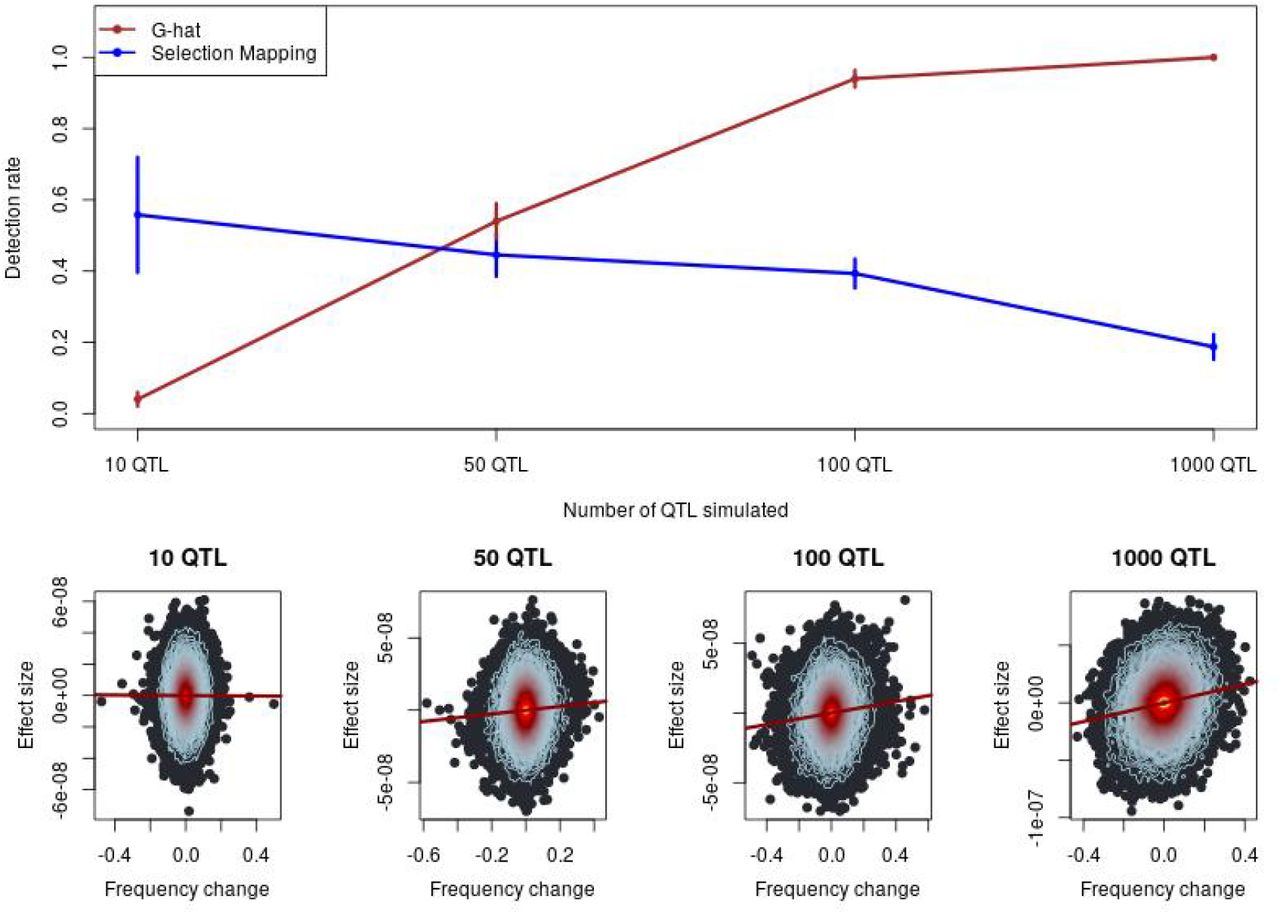
When we tested for selection in our simulated data, we observed a direct relationship between the number of QTL controlling a trait and the power of Ĝ to identify selection on that trait. Ĝ powerfully identifies selection on highly polygenic traits, but is not powerful for identifying selection on traits controlled by a small number of QTLs. Analyses of the same simulations using FST-based selection mapping showed that traits controlled by a small number of QTLs can be mapped using traditional selection mapping approaches. However, as traits become increasingly polygenic, our simulations demonstrate that the ability to map individual selected genes diminishes (Figure 1). These findings demonstrate how Ĝ and traditional mapping are complementary depending on the underlying genetic architecture of a trait. Table 1 depicts detection and false positive rates for Ĝ and FST-based mapping under different genetic architectures.

The power of Ĝ to identify selection. Top: The detection rate of Ĝ compared to Fst-based selection mapping. Vertical lines indicate one standard deviation. Standard deviations for selection mapping were estimated empirically. Standard deviations for Ĝ were estimated based on the binomial distribution. Bottom: Exemplary heat plots depicting individual-SNP allelic effect estimates linearly regressed on allele frequency change over time. Each point represents a SNP, while the contour lines indicate the density of SNPs. From the regression line, observe that a stronger relationship between frequency change and effect size corresponds to increasing polygenicity.
Detection and false positive rates for Ĝ and Selection mapping. One Ĝ test is conducted per simulation, so true and false positive rates are shown. For selection mapping, one test is conducted per marker in each simulation, so the mean number of markers that were declared true and false positives is shown. A marker was declared a false positive in selection mapping if it exceeded a 5% simulation-based experiment-wide significance threshold but was not within a .1 cM region around a simulated QTL.
Selection on maize silage traits
We re-analyzed data from a previous study that tested for selection in a decades-long breeding program for maize silage quality (Lorenz et al. 2015). Very briefly, a selection index comprised of experimentally-measured traits related to silage quality was used to perform reciprocal recurrent selection for breeding improved maize. Traits comprising the index included acid detergent fiber (ADF), protein content, starch content, in-vitro digestibility, and yield (www.cornbreeding.wisc.edu). In total, 648 individuals from various stages of selection were genotyped. Between 240 and 300 of these individuals were also phenotyped, depending on the trait. Selection mapping (Wisser et al. 2008) was previously performed utilizing simulations of drift to scan for selection, but the analysis did not identify any loci that showed significant evidence of selection. This is in spite of quantifiable improvement of the population and demonstrated heritability of the index-composing traits (Lorenz et al. 2015). We re-analyzed the same data to evaluate evidence for polygenic selection on the measured traits, which included NDF, in-vitrodigestibility, crude protein content, starch content, yield, and dry matter. After filtering, these data consisted of 10,023 polymorphic markers. Due to the relatively small population size and recurrent selection breeding scheme, we expect slow LD decay and therefore for most of the genome to be represented with this marker set. Further analysis of LD to determine the value of Meff to utilize in our test for selection confirms this (Supplemental Figure 2).
Figure 2 depicts the maize patterns of selection that were observed in our analysis. In these plots, the histogram shows the null distribution of Ĝ that was observed from a permutation test, while the vertical line depicts the observed value of Ĝ when applied to the experimental data. We observed that with the exception of protein, for the traits where we had an a priori expectation of selection, we not only identified that selection did occur, but we correctly estimated the direction of selection (positive or negative) from the data. One of the traits measured was silage dry matter (DM), which was not a part of the selection index. We did not identify evidence of selection on DM, as was expected.

Evidence of selection for maize silage traits. For six traits, the relationship between estimated allelic effects at individual SNPs and the change in allele frequency over generations is plotted. The red line is a regression of effect size on allele frequency change. Contour lines indicate the density of points, with blue contours indicating fewer points than red. Inset plots depict observed values of Ĝ (blue lines) and their statistical significance based on a comparison to permuted null distributions (red densities) for no-selection scenarios. An exact two-sided p-value is given within each inset. Significant values of Ĝ above the permuted mean indicate selection operated in the positive direction, while significant values below the permutation mean indicated selection operated in the negative direction.
Selection on chicken traits
We tested for evidence of selection in two panels of commercial lines of laying hens: one white layer (WL) and one brown layer (BL). Both closed lines have been selected over decades with a similar composite breeding goal, comprised of laying rate, body weight and feed efficiency, egg weight, and egg quality, among other objectives. The respective weights applied to the different traits varied between lines and over time. Traits analyzed included laying rate, egg weight, and breaking strength of eggs. Genotypes were available only for the post-selection population, so initial allele frequencies were inferred based on pedigree data (Gengler et al. 2007). Mind was determined based on separate evaluations of LD in the WL (Supplemental Figure 3) and BL (Supplemental Figure 4) populations.
Among the traits evaluated, we observed significant evidence of selection for increased laying rate in both WLs (p = 0.027) and BLs (p =0.0193). Tests were also suggestive of selection for increased eggshell breaking strength in WLs (p < 0.1; one-sided p < 0.05), while there was no evidence of directed selection for egg weight (Figure 3). To verify that these results were not driven by a small number of SNPs with high estimated effect sizes, we repeated the analysis with the 10 largest effect-size SNPs removed and saw virtually identical results (Supplemental Figure 5). The result for egg weight can be seen as a ‘negative control’ since for this trait an optimum value is already achieved and maintained by balancing selection. The fact that we were not able to detect significant evidence of selection in a trait such as eggshell breaking strength in both lines (although a tendency can be observed) may be due to the fact that improving those traits is part of a complex multi-objective breeding program, or simply that our test was underpowered for these traits. The unavailability of experimentally-estimated initial frequencies and our alternative use of pedigree-inferred initial allele frequencies likely weakened the power of the test as compared to the more complete data available for maize and in the simulations.

Evidence of selection for chicken traits. For three traits in white (left column) and brown (right column) laying hens, the relationship between estimated allelic effects at individual SNPs and the change in allele frequency over generations is plotted. The red line is a regression of effect size on allele frequency change. Contour lines indicate the density of points, with blue contours indicating fewer points than red. Inset plots depict observed values of Ĝ (blue lines) and their statistical significance based on a comparison to permuted null distributions (red densities) for no-selection scenarios. An exact two-sided p-value is given within each inset. Significant values of Ĝ above the permuted mean indicate selection operated in the positive direction, while significant values below the permutation mean indicated selection operated in the negative direction.
Discussion
We have defined a test statistic, Ĝ, that combines phenotypic and genotypic information to test for selection on traits controlled by many loci of small effect. The approach utilizes estimated effect sizes for individual loci and allele frequency changes over time resulting from selection on those loci. Therefore, Ĝ is most applicable in experimental or breeding populations, where both pieces of information are readily available via genotyping individuals from multiple generations. However, phenotypic information for estimating allelic effects is only required from a single time-point, so this approach can be applied post-hoc using DNA samples from previous generations even if phenotyping is no longer possible. As the practice of sequencing ancient DNA from archeological sites, museum samples, or other sources becomes progressively commonplace (Orlando et al. 2015), we envision that this approach may become increasingly applicable for ecological questions, evolutionary studies, and for human research.
Powerful for highly quantitative traits
Methods for mapping genes associated with important traits or for identifying loci that are under selection are most powerful for large-effect genes. A simple explanation for the disappointing number of associations that have been uncovered to date through GWAS is that complex traits are often controlled by many genes of small effect (Yang et al. 2011). If this is the case, enormous sample sizes are required to map loci regardless of the methodological enhancements that can be applied. Human geneticists have had success studying complex traits by utilizing extremely large sample sizes (Rietveld et al. 2013; Wood et al. 2014). But, sample sizes of this magnitude are not yet achievable within resource limitations for most species, and, arguably, will never be. Conversely, population genetic studies aiming to scan for selection have been most successful at identifying hard sweeps, where a new mutation of large effect rapidly rises to fixation as a result of selection (Pritchard et al. 2010). Only few methodologies with limited power exist for mapping soft sweeps, when the beneficial allele is already at intermediate frequency at the start of selection (Garud et al. 2015); Ma et al. 2015). A likely explanation for the presence of soft sweeps is that they often result from loci of small effect increasing in frequency slowly in a population and therefore existing on multiple distinct haplotypes or mutating multiple times before fixation. In an agricultural context, many soft sweeps may be due to newly defined breeding goals which put selection pressure on genes that previously were segregating in the populations, but were selectively neutral. The Ĝ statistic does not attempt to map specific genes— instead it pools information from all SNPs to test for selection on specific traits. This approach completely avoids the question of which loci are associated with a trait. Instead of testing each SNP, we perform one test based on information from all SNPs. Therefore, a strong statistical signal arises when a large proportion of SNPs behave similarly but not when a few SNPs portray strong signals on their own.
It was recently argued that most complex disease traits in humans are controlled by small-effect genes dispersed throughout the genome – the omnigenic hypothesis (Boyle et al. 2017). Likewise, many important traits in agricultural animal and plant species tend to be quantitative in nature and are presumably controlled by small-effect genes (Goddard and Hayes 2009; Wallace et al. 2014). For these agricultural organisms, geneticists and breeders have long recognized the benefits that can be achieved by predicting breeding values and/or phenotypes based on models that use all SNPs simultaneously (Meuwissen et al. 2001; Heffner et al. 2009; Goddard and Hayes 2009). In fact, the development of these models has led to dramatic re-designs of modern breeding protocols (Schaeffer 2006; Cabrera-Bosquet et al. 2012). The Ĝ statistic represents one avenue to leverage information from all measured SNPs to gain an understanding of the evolutionary history of a population. This approach is analogous to genomic selection/prediction as utilized by animal and plant breeders, with an important distinction: instead of predicting breeding values to determine which individuals should be selected for the future, it utilizes genotypic frequencies over time coupled with phenotypic information to unravel the history of selection in the past.
Genotypes from base population provide high power
Compared to other methods that test for selection on quantitative traits (Berg and Coop 2014; Zeng et al. 2017), Ĝ is unique in that it leverages genotypic information from multiple time points and that it incorporates information from all SNPs instead of restricting to a previously identified set of SNPs from one or multiple independent GWAS’s. With the exception of a few traits in heavily studied species, such as human height (Wood et al. 2014), few species, if any, provide the enormous sample sizes required to implicate a large number of loci for any quantitative traits. This includes situations where scientists are reasonably certain that a genetic architecture consisting of small-effect loci persists. Importantly, Ĝ is powerful because of the independence of the estimation of allele frequency changes across generations and effect sizes, respectively. Even when allelic effects and/or allele frequency changes are small, they cumulatively generate a powerful test since they can be compared across all genotyped loci. However, our analysis of the chicken data suggested that the power of the test can be reduced through noisy estimation of allele frequency change. Our reliance on pedigree data to derive initial allele frequencies was not as precise as the direct measurement of initial allele frequencies that was conducted for maize. Although we were still able to find evidence of selection on traits including laying rate, which was almost certainly under the strongest selection, there were selected traits we did not detect potentially due to this noise.
Future directions and conclusions
We have developed an approach to test for selected traits that avoids the preliminary identification of candidate genes or regions. The approach is particularly applicable in experimental, agricultural, and natural populations for which available resources dictate limited sample sizes for conducting massive mapping studies for such preliminary identification. In contrast to purely population-genetic analyses, which rely solely on genotypic information, our methodology requires that phenotypic data be collected on at least one time-point of genotyped individuals. Additionally, multiple time-points of genotypic information are needed, either directly or through pedigree-based imputation.
While the Ĝ statistic is most directly applicable for the discovery of traits that have been previously under selection during recent evolution, it may have additional applications. Recent studies have demonstrated that distinct physical regions of the genome, such as individual chromosomes, often contribute a disproportionate amount to trait variance (Bernardo and Thompson 2016). Rather than applying the Ĝ statistic genome-wide, future research should be conducted regarding whether it can be applied across any collections of loci such as individual chromosomes, pathways, gene-families, functional classes, or other categories to test if these show evidence of selection on a quantitative trait. This would represent a process allowing researchers to map significant features as opposed to genes.
Although Ĝ does have potential as a tool for mapping categories of selected loci, the simple identification of traits that have been under selection may prove enormously useful. Whether agricultural, experimental, or natural, it is often difficult to determine all of the traits that are advantageous in a population or respond to natural or anthropogenic selection, including undesired selection responses. The application of the Ĝ statistic genome-wide allows this determination, which may help scientists select the right traits for maximum agricultural production, determine inadvertently selected lab traits impacting experimental outcomes, and establish ecologically important traits for survival in the wild.
Materials and methods
Simulations
Each simulation started with a random mating historical population. After 5 thousand generations, selection began and simulations proceeded with more control over each generation. Truncation selection was performed based on high phenotype. Drift simulations were identical to selection simulations in terms of genome layout and genetic basis of the trait, but individuals were selected randomly. Simulations were performed with QMSim (Sargolzaei and Schenkel 2009). Parameters for simulations are provided in full in Supplemental Table 1.
Selection mapping in simulations
Pre- and post-selection simulated allele frequencies were output from QMSim. These were used to calculate marker-specific FST values, as was performed by (Lorenz et al. 2015). FST was computed according to  , where s2 is the sample variance of allele frequency between pre- and post-selection populations, and
  is the mean allele frequency (Weir and Cockerham 1984). Experiment-wide 5% significance threshold were identified based on the 95% FST quantile observed from drift simulations. These thresholds were applied to FST values obtained from selection simulations to determine detection and false positive rates. Simulated QTL were declared detected if a significant marker was identified within a .1 cM window surrounding the QTL. False positives were defined as markers that were not within a .1 cM window surrounding any simulated QTL.
Maize data
All maize data were previously published and described by Lorenz et al. (2015). In brief, a selection index comprised silage-quality traits was used to perform reciprocal recurrent selection. Traits comprising the index were yield, dry matter content, neutral detergent fiber (NDF), protein content, starch content, and in-vitro digestibility (www.cornbreeding.wisc.edu). Phenotypic data included five cycles of selection, encompassing approximately 20 generations in total. Tens to hundreds of individuals were sampled from each cycle of selection to be genotyped. Genotyping was performed with the MaizeSNP50 BeadChip, which includes 56,110 markers in total (Ganal et al. 2011). After removing monomorphic SNPs, redundant SNPs, quality filtering, and imputing, as described in Lorenz (2015), 10,023 informative SNPs remained.
Allele frequencies were computed for each cycle of selection. Because only 5 and 11 individuals from cycles 0 and 1 were genotyped, respectively, allele frequency change from cycle 2 (n = 163) to cycle 5 (n = 211) was computed for each SNP. Since all SNPs were di-allelic, the frequency of only one allele was tracked, and the frequency change for that allele perfectly mirrored the change for the other allele. For the tracked allele only, allelic effects were estimated using the R package RR-BLUP (Endelman 2011). Phenotypic information was available from individuals representing selection cycles 1 through 4. Therefore, a fixed effect for cycle was included in our model. Our exact analysis scripts are available at github.com/timbeissinger/ComplexSelection.
Chicken data
Data were available for one white layer (WL) and one brown layer (BL) line from a commercial breeding program. Both closed lines have been selected over decades with a similar composite breeding goal, comprising, among others, laying rate, body weight and feed efficiency of the hens, as well as egg weight and egg quality, where the respective weights of the different traits varied between lines and over time. In total, 673 (743) WL (BL) individuals were genotyped, of which > 80% were from the last generation and the remaining animals were parents, grand-parents, and great-grandparents of the actual birds. For all genotyped individuals, complete pedigree data were available comprising 2109 (1879) individuals and going 13 (9) generations back in WL (BL). The oldest generation was defined as the base population and comprised 111 (64) ungenotyped individuals being separated from the majority of genotyped individuals by 12 (8) generations.
Current individuals were genotyped with the Affymetrix Axiom® Chicken Genotyping Array which initially carries 580K SNPs. This data were pruned by discarding sex chromosomes, unmapped linkage groups, and SNPs with minor allele frequency (MAF) lower than 0.5% or genotyping call rate smaller than 97%. Individuals with call rates smaller than 95% were also discarded. Subsequently, missing genotypes at the remaining loci were imputed with Beagle version 3.3.2 (Browning and Browning 2009),resulting in sets of 277’522 (334?43) SNPs for the WL (BL) individuals.
To calculate the allele frequency change in the chicken populations, the allele frequency in the base population individuals had to be reconstructed by statistical means. This was done with the approach of Gengler et al. (2007), which, in short, considers the allele frequency in an individual as a quantitative and heritable trait and uses a mixed model approach to obtain a best linear unbiased prediction (BLUP) for the allele frequency of all un-genotyped individuals. This is done by linking the genotyped offspring to the un-genotyped ancestors via the pedigree information (for details, see Gengler et al. 2007). This required solving 277’522 (334’43) linear equation systems of dimension 2109 (1879) for the WL (BL) data set. Next, Δi for locus i was calculated as the difference of the observed allele frequency of the genotyped individuals in the current and the 3 ancestral generations and the average estimated allele frequency of the 111 (64) base population individuals 12 (8) generations back.
For each genotyped individual, conventional (non-genomic) BLUP breeding values and the respective reliabilities for a wide set of traits were available. SNP effects were estimated in a two-step procedure: first, for each trait in each line genomic breeding values were estimated via genomic BLUP (GBLUP), followed by a back-solution of estimated SNP effects. In the GBLUP step, the model y = 1μ + Zg + e, was solved, where y is the vector of de-regressed proofs DRPs of genotyped individuals for a specific trait; μ is the overall mean; g is the vector of additive genetic values (i.e. genomic breeding values) for all genotyped chickens; e is the vector of residual terms; 1 is a vector of 1s and Z is a squared design matrix assigning DRPs to additive genetic values with dimension number of all genotyped individuals. Residual terms were assumed to be distributed  , where R is a diagonal matrix with diagonal elements
  (Garrick et al. 2009) for an individual i in the training set, where
  is the reliability of DRP for individual i,
  is the residual variance, using c set to 0.1. The distribution of additive genetic values is assumed to be
  , where
  is the additive genetic variance and G is a realized genomic relationship matrix which was constructed according to (VanRaden 2008). Estimation of variance components and genomic breeding values was done with ASReml 3.0 (Gilmour et al., 2009).
Next, estimated SNP effects ŝ were obtained following Strandén and Garrick (2009) as
 where M is a matrix of dimension number of genotyped individuals x number of genotyped SNPs with entry mij = xij − 2pj where xij is the genotype of individual i at locus j (coded as 0, 1, or 2 which are counts of the reference allele) and pj is the population frequency of the reference allele at SNP j.
Computational Resources
Computation was performed using the University of Missouri Informatics Core Research Facility BioCluster (https://bioinfo.ircf.missouri.edu/). Computational nodes where simulations were performed had 64 cores and 512 GB of RAM.
Data availability
Maize data are available in from Lorenz et al. (2015). Chicken data, including allele frequency change and estimated SNP effects, will be made available on Github or Figshare upon publication. All scripts used for simulations and analysis are available at github.com/timbeissinger/ComplexSelection.
Acknowledgements
We thank Natalia de Leon, Aaron Lorenz, and Lohmann GMBH for generating the maize and chicken biological data used in this study. We are grateful for helpful discussions with Emily Josephs and Aaron Lorenz. This research was supported by the USDA Agricultural Research Service, CRIS project number 5070-21000-038-00-D.
References


