

ABSTRACT
Variance in reproductive success is a major determinant of the degree of genetic drift in a population. While many plants and animals exhibit high variance in their number of progeny, far less is known about these distributions for microorganisms. We quantified the distribution of descendants arising from stochastically germinating Streptomyces spores by applying a novel and generalizable method. The distribution is heavy-tailed, with a few cells effectively “winning the jackpot” to become a disproportionately large fraction of the population. This not only decreases the effective population size by many orders of magnitude but can lead to its sub-linear scaling with the census population size. Furthermore, incorporating the empirically determined distribution into population genetics simulations reveals allele dynamics that differ substantially from classical population genetics models with matching effective population size. These results demonstrate that stochastic exists from dormancy can have a major influence on evolution in bacterial populations.
INTRODUCTION
Since the dawn of population genetics, it has been clear that the distribution of the number of offspring per parent is central to developing a quantitative understanding of the evolution of genetic variants (1–5). The offspring distribution provides a mapping between generations and directly determines the extent to which genetic drift affects allele frequencies in a population (6). Specifically, the effective population size, which is often used to quantify genetic drift, is inversely proportional to the variance of the offspring distribution. In classical models of population genetics, such as the Wright-Fisher model, the offspring distribution is Poisson distributed (7, 8). However, for some animals there is high variance in reproductive success, with a minority of males fathering a large fraction of the children in each generation (9–12). Such highly-skewed offspring distributions have fundamental implications for how we predict and interpret fluctuations in allele frequencies (6, 13, 14). These implications include: dramatic (e.g., six orders of magnitude) discrepancy between census and effective population size (13), genetic patchiness on small spatial scales despite long-range dispersal (12, 15, 16), and dramatically altered effectiveness of selection compared with classical population genetics models (6, 17, 18).
In contrast to plants and animals, the offspring distribution is largely unexplored for microorganisms. One reason for this might be that the offspring distribution is seemingly simpler for bacteria undergoing binary fission, since each cell can only leave behind 0 (death), 1 (no doublings), or 2 descendants. However, even clonal populations of bacteria display a distribution of growth rates and lag times, causing them to yield a variable number of offspring after some time (19–22). In particular, many microorganisms form spores or persister (non-growing) phenotypes to survive unfavorable environments or disperse (19, 23, 24), and exit from dormancy is often a stochastic process that presumably evolved as a bet hedging strategy to overcome environmental uncertainty (20, 25).
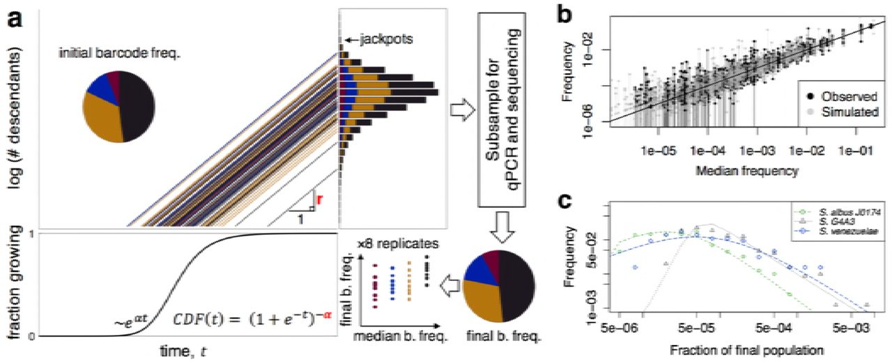
Importantly, it is unclear how stochastic variability in growth rates and lag times affects genetic drift. One way to study this quantitatively is by examining the distribution of the number of bacteria arising from a single bacterium after a given amount of time τ, where the time τ is substantially longer than the standard doubling time (Fig. 1a). This is a stochastic quantity which can be described by a probability distribution that we term here the ‘distribution of descendants’. In a system with seasonality, for example, one might look at this distribution after one season. Defined as such, the distribution of descendants is a fundamental quantity of which little is known for bacteria. Quantifying this distribution and how it varies across species and environments would likely improve our understanding of genetic drift in microbial populations and, ultimately, our ability to correctly interpret the genetic variability observed in sequence data.

a, Clonal cells, represented by colored circles, are grown for a period of time (τ) before their relative abundances are measured. b, The variability in the proportion of descendants between replicate populations of cells is used to determine the distribution of descendants. c, The distribution of descendants may take on a variety of shapes that have different rates of converging to zero. A heavy-tailed distribution (solid line) would result in "jackpots" where individuals have much greater reproductive output than expected based on their initial frequency. d, In order to track lineages, we constructed a barcoded library of Streptomyces where each spore has a unique 30 base-pair lineage-specific sequence integrated into its chromosome.
Here we present a scalable methodology for quantifying the distribution of descendants in clonal populations. We used a generalizable barcode tagging approach that enabled us to track descendants from hundreds of sub-populations differing only by a short DNA barcode inserted in their chromosome. We developed two analysis methods for determining the distribution of descendants from barcode data, and applied these approaches to soil bacteria from the genus Streptomyces. We focused on Streptomyces because they have complicated life-cycles, and the impact of life-cycle stages on the distribution of descendants is particularly poorly understood (26). Using the variability between replicates, we show that the distribution of descendants is heavy-tailed – that is some bacteria represent a far greater proportion of the final population than their initial frequency. Furthermore, using microscope time-lapse imaging, we demonstrate that the heavy-tailed nature of the distribution of descendants can, in our case, be largely explained by phenotypic variability in lag time before exponential growth. We then examine the implications of heavily-skewed distributions of descendants for the population genetics of microorganisms.
RESULTS
High-throughput measurement of the distribution of descendants
Directly determining the distribution of descendants would require tracking each individual cell and all of its offspring within a clonal population. Such a brute force strategy is exceedingly difficult, if not impossible. Therefore, we developed an alternative method to track sub-populations of cells and infer the shape of the distribution of descendants based on changes in the relative abundance of sub-populations between replicates (Fig. 1bc). This method involves tagging bacterial lineages of an otherwise clonal population with a unique 30 base-pair random sequence inserted at a fixed site on the chromosome (Fig. 1d). A similar technique has been used previously to tag yeast and Escherichia lineages (27, 28). After barcoding, we grew 5 different strains of Streptomyces in 8 separate replicate populations starting from 3 different initial concentrations. Streptomyces strains first germinate and then grow as interconnected filamentous colonies within liquid medium. After 7.5 days of growth, genomic DNA was extracted and the barcoded region was amplified before sequencing (see Methods). We observed between 211 and 2,534 unique barcoded lineages per strain across all replicates in the experiment. An example of the data collected for one of the five strains is depicted in Fig. S1.
Since our analysis methods are based on the variability between replicate populations, they require that the technical variability due to the experimental procedure be far less than the biological variability. To investigate both of these components of variability, we compared the frequency distribution determined from technical (PCR) replicates to that originating from distinct biological replicates. We found that technical replicates had substantially higher correlation than biological replicates (Fig. S2), confirming that most of the variability is biological in nature. This allows the shape of the distribution of descendants to be inferred from fluctuations in the relative abundance of barcodes between biological replicates. However, it is worth noting that we can only observe the right side of the distribution of descendants, because the lower detection limit of our method is approximately 1 in 105 cells based on the number of initial templates in PCR and sequencing reads. Therefore, we would not observe the rarest barcodes if they decrease in relative frequency substantially during the course of the experiment. Nonetheless, we are most interested in the right-tail of the distribution of descendants because it might include lineages that increase considerably in relative abundance.
The distribution of descendants is skewed with a heavy tail
Two extremes of the barcode frequency distribution across replicates reveal characteristics of the distribution of descendants (Fig. 2a). At one end, the abundance of a barcode present at high frequency is expected to be normally distributed across replicates. This is because, for abundant barcodes, each barcode represents a large number of initial cells and the final barcode frequency is a sum of many realizations of the distribution of descendants. Based on the central limit theorem, the variation across replicates will approach normality, so long as the underlying distribution of descendants has a tail that decays sufficiently fast. We tested whether the relative frequencies of the 8 replicates belonging to the most abundant barcodes could be normally distributed using the Shapiro-Wilk test. Each of these barcodes is estimated to be shared by over 1,000 initial cells per replicate. For 4 out of 9 of these abundant barcodes the normal distribution was rejected with p-value < 0.02 (Fig. 2b). Moreover, the fact that we could repeatedly reject a normal distribution even with a small number of replicates indicates that the deviations from normality are strong. Thus, this analysis suggests that the underlying distribution of descendants is heavy-tailed.

a, Barcodes at the two extremes of relative abundance reflect the shape of the distribution of descendants. b, Abundant barcodes, those shared by more than 1000 cells in the initial population, are expected to converge to a normal distribution due to the central limit theorem. However, many of the most abundant barcodes were not normally distributed across replicates, based to their p-values (at right) in the Shapiro-Wilk test. Instead, the abundant barcodes originating from three different strains (colors) were widely scattered in terms of their final proportion of the population (x-axis). c, The singletons, those barcodes occurring in only 1 out of 8 replicates, approximate the shape of the distribution of descendants since they likely started from single cells. For the strain with the most singletons, Streptomyces G4A3 (808 singletons), we observed that their relative abundances at the end of the experiment were more heavy-tailed than a fitted log normal distribution (green curve). The outlying “jackpots” represent cells that grew to a far higher abundance than the median abundance of singletons, in many case by more than 100-fold. Note that the left-side of the distribution is likely truncated because it contains barcodes that fall below the lower detection limit of our method.
At the other extreme, as the initial frequency of a barcode approaches a single cell (Fig. 2a), the distribution of final barcode frequencies should approximate the distribution of descendants. We made the approximation that barcodes appearing in only 1 out of 8 replicates of a given initial concentration were sufficiently rare to have originated from a single cell. While we would expect this assumption to be violated in about 10% of cases, the impact of starting from 2 cells should be on the order of 2-fold. The resulting distribution of barcode frequencies for these “singletons” is heavy-tailed and appeared broader than a log-normal distribution (Fig. 2c). Surprisingly, for many strains the distribution spanned over three orders of magnitude, meaning that some barcodes were over-represented by more than 1000-fold that of a typical barcode starting from an identical initial frequency (Fig. S3).
While the singleton distribution provides a model-free estimate of the distribution of descendants, the downside of this approach is that it only uses a subset of the data, and it requires the presence of many rare barcodes. For example, one of the barcoded strains, S. S26F9, had a diversity of barcodes, but only six were at low enough frequency to be observed in a single replicate (Fig. S3c). Correspondingly, we wondered whether it would be feasible to develop a more statistically robust procedure for determining the distribution of descendants by fitting a growth model to all of the data points for each strain.
Stochastic exits from dormancy largely explain the heavy-tail
In order to develop a model for fitting the entire dataset, we first needed to establish the major sources of growth variability among Streptomyces cells in a population. We reasoned that growth variability would largely result from two sources: differences in lag time before growth (driven by variability in germination times) or variability in growth rates that is auto-correlated across divisions. To determine which source dominated growth variability in our experimental system, we tracked strains under a microscope during their first day of growth on agar medium containing the same nutrients as the liquid experiment. This resulted in large images (Fig. 3a) that we aligned between time points to track the growth of each germinated spore (see Methods). Colony growth was constrained to two dimensions for a long time, which allowed us to estimate the number of genomes present from the area covered by the colonies. This method provides a means of directly assessing the distribution of descendants until the time the colonies intersect and can no longer be distinguished.

a, A vertical cross-section representing one-fifth of a composite image of S. S26F9growth after 22.4 hours on solid medium with regions shown in (b) denoted by white boxes. b, Colonies originating from single spores can be drastically different in size at the same point in time. The image on the left shows the largest non-intersecting colony after 22.4 hours of growth. The two images on the right highlight the smallest identifiable colonies (circled) at the same time point and scale. The colony on the left has approximately 330 times more mycelial area than either of the colonies on the right. c, Growth curves for 301 colonies of S. S26F9 tracked under the microscope. Each line represents the mycelial area of a colony originating from a single spore, and the lines are truncated when colonies intersect. Since mycelium thickness is approximately constant, this measure is proportional to the total length and volume of the mycelium filaments. The largest colonies had a mycelia area almost 3-orders of magnitude greater than the smallest colonies at the end of the experiment.
Three of the five strains mostly completed germination during the course of the experiment, while two strains germinated too late to adequately track under the microscope. All three early-germinating strains displayed wide variation in colony size after one day of growth, with the largest colonies being almost 3-orders of magnitude larger in biomass than the smallest (Fig. 3b, Fig. S4). This likely underestimated the extent of variability, as large colonies can easily overwhelm smaller colonies so that they cannot be identified at later time points and because we sampled only hundreds of spores, thus missing rare instances of early germination. Nevertheless, it was clear that variation in germination times might largely account for the extreme variability observed in the distribution of descendants. Such lag time variability in Streptomyces has recently been shown to be a phenotypic effect rather than a genotypic effect (20). After germination, the colonies grew in size deterministically at nearly the same rate (Fig. 3b, Fig. S4). However, it is possible that minute differences in growth rate could compound the initial variability to make the distribution even wider at time points beyond the duration of colony tracking. Overall, the result from the time-lapse microscopy revealed that the growth of our Streptomyces strains can be partitioned into stochastic germination and deterministic growth for the utilized growth media.
Fitting the entire dataset supports distributions of descendants with fatter than log-normal tails
Based on the microscope data, we constructed a model in which we partitioned growth into two phases: an initial lag time drawn from a distribution, followed by exponential growth at a fixed rate common to all cells. We wished to determine whether a model based on variability in germination times alone could adequately recapitulate the entire dataset and, if so, determine the distribution of descendants through parameter fitting without limiting ourselves to the subset of the data representing rare barcodes. To this end, we simulated the entire experimental process, starting from sampling an initial population of barcodes, then “growing” each barcode according to the aforementioned growth model, and sampling the resulting barcode frequencies for PCR amplification and sequencing steps (Fig. 4a). Since we know the initial census population size from plate counting, the number of initial templates per replicate based on quantitative PCR, and the number of reads obtained in sequencing, the entire simulation depends only on the shape of the distribution of lag times relative to a time scale set by the fixed exponential growth rate. Since the fraction of germinated spores as a function of time follows a sigmoidal curve (20), we compared two families of commonly used sigmoidal curves: the generalized logistic function and the cumulative distribution function of the skew normal distribution, which respectively lead to power-law and log-normal tails for the distribution of descendants (Fig. S5).

a, We performed simulations of the entire experiment with different distributions of descendants to test their ability to recapitulate the observed data (see Materials and Methods). b, The variation in relative barcode frequencies between 8 replicate populations is shown for the strain S. coelicolor at full initial concentration (black). Vertical lines connect the observed relative frequencies of each of the 8 biological replicates (points) corresponding to a given barcode, and extend to zero in cases where a barcode was not observed in one or more of the 8 replicates. Simulation results (gray) closely mirror the observed data. c, The optimal distributions of descendants obtained from parameter fitting (colored lines) generally matched the relative frequencies of singletons (points) for the three strains with the most singletons: S. albus J1074 (400 singletons), S. G4A3 (808), and S. venezuelae (64).
Each of the two sigmoidal families was controlled by two parameters, r and α, that allow independent adjustment of the distribution of descendants’ width and skew (i.e., left-right asymmetry) (Fig. 4a). We used the results of 1000 simulations to quantify the fit of each parameter combination that was tested (Methods). Briefly, the optimality criterion (ω2) was based on the sum-of-squared differences between the cumulative distributions of the simulations and the observed data (the Cramér-von Mises criterion). The value of ω2 was calculated for many different combinations of the two parameters for the two families of germination curves (Fig. S6), and the lowest value of ω2 was selected as the optimal combination of r and α.
We found that, for 4 out of 5 species, the generalized logistic function yielded a better fit (Table S1). The two distributions only had substantially different fits in the cases with the greatest barcode diversity, suggesting that a large number of barcodes are required to adequately discern the right-tail of the distribution. Thus, in agreement with observations from singleton barcodes (Fig. 2c), the results from using all of the barcode data further support distributions of descendants with fatter than lognormal tails.
In all cases the simulations appeared to recapitulate the observed variability with high fidelity (Fig. 4b). This indicated that the simple growth model was sufficient to capture most of the variability between replicate populations. Impressively, the distribution of descendants qualitatively matched the observed singleton frequencies for the three simulated strains with the most singleton barcodes (Fig. 4c), thus providing a validation for our model-based approach for deducing the distribution of descendants by using all the barcode data. Overall, these results confirmed that variability in lag time between strains can explain the observed "jackpots", established a robust procedure for deducing the distribution of descendants, and indicated that the tail of the distribution of descendants is fatter than lognormal.
Selection is an implausible explanation for the observed distribution of descendants
A potential source of growth variation is the existence of genetic differences within the population. One genetic basis for variation is that some barcodes have pre-existing mutations that impart a higher growth rate, resulting in an exponential divergence in relative abundance over time. However, the method we used to fit the data to the simulation (Fig. 4) is unaffected by per-barcode selection coefficients because it relies on variability of fates among individuals with the same barcode. We confirmed this by incorporating selection coefficients into our stochastic simulation (see Methods) and observed negligible effect on the fitted distribution of descendants. Another way to uncover differences in inter-barcode selection coefficients is to look for correlations between the final relative frequencies of rare barcodes. We tested this by plotting the relative frequency of barcodes that were only present in 2 of 8 replicates (Fig. S7). If jackpots within this set are due to selection, we would expect them to manifest in both replicates. In contrast, the correlation between replicate barcodes was extremely low (Pearson’s r = 0.08), indicating that inter-barcode selection coefficients are not a major source of the observed variability between replicates.
These results do not rule out the possibility that there were rare individuals within a barcode lineage with new or recently acquired beneficial mutations. Such mutants would likely have had to arise after the start of the experiment in order to only be present in a minority of replicates. Given the high number of positively-skewed replicates, it is implausible that so many mutants of large effect size could occur so rapidly. Furthermore, we estimate that most cells only doubled about 10-15 times over the course of the experiment, depending on each strain’s initial concentration. Even a large growth rate advantage of 10% would be expected to result in at most a 3-fold variability in final abundances. Nonetheless, it is well known that mutation is a major cause of fitness variation in populations, and we cannot rule out the fact that some of the variance in the distribution of descendants was attributable to genetic differences.
The heavy-tailed distribution of descendants yields large deviations from classical population genetics predictions
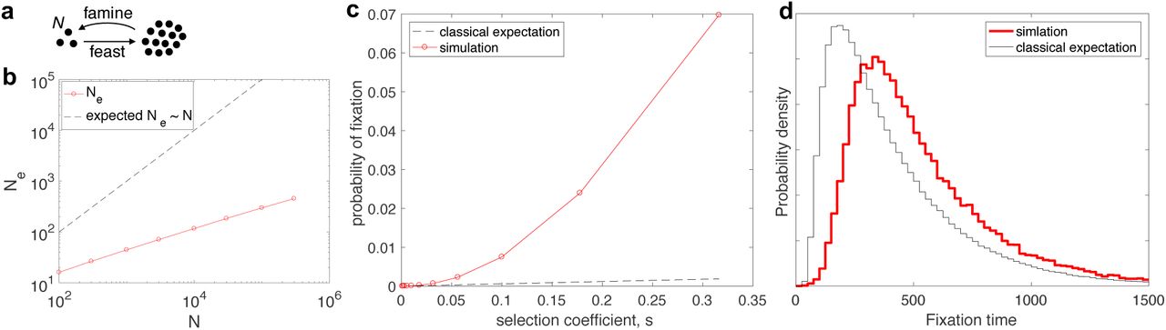
We next examined the population genetics consequences of the experimentally inferred heavy-tailed distribution of descendants through population genetics simulations. We focused on S. G4A3, for which the optimal fit was given by the generalized logistic germination curve with r = 0.2 and α = 0.28 (Fig. 4c, Table S1). We modeled a situation in which we start with N individuals, let them grow exponentially to large numbers following a stochastic exit from dormancy, and then sample N individuals at random to start the next ecological cycle (Fig 5a, Methods).

a, In the model, N individuals exit dormancy stochastically and grow exponentially at the same growth rate until a very large population size is reached. N individuals are then randomly sampled to start the next cycle. b, Shown are the variance effective population sizes (Ne) that result from simulations with different numbers of initial cells (N) (red circles connected by lines). Strikingly, Ne does not scale linearly with N (black dashed line). Instead, Ne follows a sub-linear power-law: Ne ~ Nγ with γ < 1. c, The probability of fixation is shown as a function of the selection coefficient s (red, N = 100,000, r = 0.2, α = 0.28). The classical expectation based on the formula presented in the text is shown for matching N and Ne (black dashed line). A log-log presentation of this result (Fig. S9a) reveals that, for large s, the probability of fixation is a super-linear power-law as a function of s. d, The probability of distribution for the fixation times of a neutral allele with an initial fraction of 50% is shown. The model with the experimentally determined heavy-tailed distribution of descendants is shown in red (same parameters as in b), and the Fisher-Wright model with matching effective population size is shown in black.
Through a simulation of this process, we first determined the distribution of descendants after one ecological cycle, i.e. the distribution, v(n), for the number of individuals, n, descending from one individual after one cycle. Classical population genetics theory states that the consequences of genetic drift can be captured by a Fisher-Wright model with a (variance) effective population size Ne = N / var(v). Strikingly, we found that Ne scales sub-linearly with N (Fig. 5b) for the empirically-derived distribution of descendants. That is, doubling the population size does not double the effective population size. In fact, Ne exhibited an apparent power law scaling Ne ~ N0.41. This counter-intuitive behavior stems from the fact that var(v) does not converge to a constant as a function of N (see Methods) due to the heavy-tailed nature of the distribution of descendants. Thus, even if individuals grow independently, a sub-linear scaling of Ne with N can emerge for certain distributions of lag times, which leads to a divergence between N and Ne that grows with N. This result strictly holds only for α/r < 2. For α/r > 2 or descendant distributions with lognormal tails, significant deviations from Ne~N would still occur at low N, but the proportionality between N and Ne would eventually be restored for large enough N (Fig. S8a).
The heavy-tailed distribution of descendants affects the population dynamics beyond reducing Ne (29). Through simulations, we determined the fixation probability of beneficial mutations with different selection coefficients, s. We observed (Fig. 5c) that as s increases, the probability of fixation increases much more rapidly than expected based on the classical population genetics prediction (for haploid populations) (30), which states:

In fact, the probability of fixation increases faster than linearly and follows an apparent power law as a function of s (Fig. S9a). The classical formula with matching Ne only agrees with the simulations for very small s (Fig. S9a). As a control, we verified that this formula agrees well with simulations of the Fisher-Wright model with matching Ne across the range of s values (Fig. S9b). Therefore, although the role of stochasticity is amplified for heavy-tailed distributions of descendants, it is partly counterbalanced by an increased efficiency of selection.
Finally, we examined whether purely neutral dynamics are also different from the predictions of a Fisher-Wright model with the same Ne. To this end, we computed the distribution of fixation times for a neutral allele starting at 50% abundance (Fig. 5c). We found that neutral mutations take significantly longer to fix with a heavy-tailed distribution of descendants. Thus, the population genetic dynamics resulting from the experimentally determined distribution of descendants is not captured by classical population genetic models with equivalent variance effective population size. Importantly, these deviations are generic to heavy-tailed distributions and would persist even for distributions of descendants with lognormal tails, although the magnitude of the difference would be smaller (Fig. S8b).
DISCUSSION
In this study, we developed and applied a scalable procedure for determining the distribution of descendants arising from a population of bacteria. Surprisingly, the distribution of descendants was heavy-tailed, resulting in a wide range of relative abundances after only a short time (Fig. 2). This variation was largely explained by differences in lag time before exponential growth (Fig. 3). We further showed that the observed variability in lag times and the resulting heavy-tailed distribution of descendants have non-trivial consequences for population genetics after many cycles of growth and dormancy.
This work highlights a simple and potentially common mechanism for generating heavy-tailed distributions of descendants in microbial populations. Such distributions would arise as long as the exit from dormancy is stochastic and the variation in lag times is large compared to the doubling time of actively growing cells. It is already well established that many bacteria taxa have dormancy states that allow them to persist in unfavorable environments, and in fact natural environments are often numerically dominated by dormant microorganisms (31). While there are known examples of stochastic exit from dormancy in bacteria (20, 24, 25), it is still unknown how common such stochasticity is among microorganisms. However, it has been argued, for example in the context of desert plants (32), that stochastic exit from dormancy is a bet hedging strategy that increases survival in uncertain environments. Given the generic nature of this argument, it is likely that stochastic exists from dormancy are common across the tree of life. We therefore expect that the findings described here will be relevant to many microbial populations, and will simulate further work on stochastic germination.
Quantification of this stochasticity is important not only as a means of characterizing bet hedging strategies but also for how we predict and interpret changes in allele frequencies. The functional form of germination stochasticity determines how heavy-tailed the distributions of descendants are. In particular, an exponential rise of the germination curve (Fig. 4a) can lead to fat-tailed, power-law like distributions. In contrast, a Gaussian distribution of germination times would lead to log-normal distributions, which are less extreme. Heavier tails result in greater deviations from classical population genetics predictions. One intuitive way to think about this is that the variance of a distribution no longer summarizes it well if the distribution is heavy-tailed. Thus, variance-based adjustments of the effective population size are insufficient to capture the allele dynamics. In this way, luck might play a far greater role in evolution than generally considered by classical population genetics models.
The heavy-tailed nature of the distribution of descendants is anticipated to have several effects on bacterial populations. First, extreme stochastic variability can decrease the effective population size dramatically below the census population size (13), even when the census size is measured at population bottlenecks within ecological cycles. Moreover, our experimental results supported a population genetics model in which the discrepancy between census and effective population sizes increases with the number of individuals and, therefore, becomes more important for large systems. Such processes can greatly amplify the effects of genetic drift and lead to faster elimination of genetic diversity, larger fluctuations of allele frequencies, and an increased lower-bound at which weak selective pressure can effectively act. In particular, amplified genetic drift may influence microbial population dynamics on timescales that are important to commercial biotechnologies or bacterial infections. Second, classical population genetics models with matching variance effective population size do not adequately represent dynamics in a population with a heavy-tailed distribution of descendants. We showed that the probability of fixation of beneficial mutations increases faster than linearly with the selection coefficient and that fixation times of neutral alleles are longer than expected given the effective population size. Third, since many infections are caused by a small initial number of cells or viruses, wide distributions of descendants may greatly influence the early burden on the host and partly explain the variability in symptoms observed between patients with the same infection. Finally, our results offer support for the notion that true fitness, that is the long-term propensity to have more descendants, is difficult to measure (33). Even the largest sub-populations in our experiments exhibited variability in their relative abundance between replicates due to jackpots. Owing to insufficient replication or low initial population size, this variability could easily be interpreted as a long-term heritable fitness difference when potentially none is present.
While, to our knowledge, this is the first measurement of a distribution of descendants for bacteria, it is known that viruses also exhibit large variation in the number of progeny generated from each infected cell. For example, human cells can differ by up to 300-fold in the number of released viruses depending on the stage of the cell cycle in which the infection occurs (34, 35). The methodology employed here for tracking Streptomyces could be extended to study the distributions of descendants for other species and environments. It would be particularly interesting to determine the distribution of descendants of bacterial populations in their natural environment or as part of the human microbiome, where additional complexities might further broaden the distribution relative to the homogeneous environment explored in this study.
MATERIALS AND METHODS
Construction of barcoded strains of Streptomyces
Oligonucleotides 5’-GATCCACACTCTTTCCCTACACGACGCTCTTCCGATCT-3’ and 5’-S20-N30-AGATCGGAAGAGCGTCGTGTAGGGAAAGAGTGTG/3Phos/ were purchased from Integrated DNA Technologies. The latter oligonucleotide is different for each strain library and contains a unique 20-nucleotide strain barcode (S20), a stretch of 30 random nucleotides that form the set of lineage barcodes (N30), and a 3’-phosphate modification. To permit robust identification of a strain in the presence of sequencing errors, the S20 sequences were designed using EDITTAG (36). The 34-nucleotide complementary region of the two oligonucleotides were annealed, made double stranded using Klenow Polymerase (Promega), and then modified using T4 Polynucleotide Kinase (New England Biolabs), which removes the 3’-phosphate and adds 5’-phosphates. Subsequently, this DNA insert was ligated into plasmid pSRKV004 cut with BamHI and EcoRV (New England BioLabs). The plasmid pSRKV004 is a derivative of the integrating plasmid pSET152 (37) in which the orientation of EcoRV and BamHI sites in the multiple cloning site is reversed.
To reduce the background of pSRKV004 without inserts after ligation, the ligation mixture was digested with EcoRV and NotI (New England BioLabs) and then transformed into E. coli 10G ELITE cells (Lucigen) via electroporation. Transformants were selected on lysogeny broth (LB) plates with 50 μg/ml Apramycin, and the pool of transformants underwent plasmid preparation (miniprep) using a commercial kit (Promega). The miniprep was again digested with EcoRV and NotI and the resulting library was introduced into the conjugation helper strain ET12567-pUZ8002 (37) via chemical transformation. Transformants were selected on LB + 15 μg/ml Chloramphenicol + 50 μg/ml Kanamycin and 50 μg/ml Apramycin plates, pooled, and grown in liquid LB containing 15 μg/ml Chloramphenicol, 50 μg/ml Kanamycin and 50 μg/ml Apramycin for 2-3 hours in a 37°C shaker.
This E. coli culture was used for conjugation into the desired Streptomyces strain according to a standard protocol (37). Briefly, the transformed conjugation helper strain was mixed with Streptomyces spores, the bacterial mix was grown on mannitol-salt (MS) agar for 16 hours and then overlaid with Apramycin (100 μg/ml) and Nalidixic acid (50 μg/ml). Strains successfully undergoing conjugation integrate the plasmid at a phage attachment site in their genomic DNA (38). Barcoded libraries were prepared by scraping spores from exconjugants and selecting against E. coli carryover by propagating the spores on Streptomyces Isolation Medium (37) supplemented with 50 μg/ml Nalidixic acid and 100 μg/ml Apramycin for two growth cycles.
Strains and growth conditions
Five barcoded Streptomyces strains were chosen based on having more than 100 distinct barcodes per strain. These five strains were S. coelicolor, S. albus J1074, S. G4A3 (39), S. S26F9 (40), and S. venezuelae. Across all experiments, we observed a total of 283, 1611, 2534, 211, and 419 unique N30 barcodes, respectively, for the 5 strains. Full concentration spore stocks were diluted 10-fold and 100-fold to generate three initial concentrations, and aliquoted into 8 replicates per concentration, each containing a single strain (120 total populations). Each replicate (30 μl) was used to inoculate 1 ml of 1/10th concentration ISP2 liquid (10 g Malt extract, 4 g Yeast extract, and 4 g Dextrose per 1 L) in a sterile 1.5 ml polystyrene tube (Evergreen Scientific). A small hole was made in the cap of each tube to allow air flow. Tubes were incubated for 7.5 days at 28°C while shaking at 200 rpm.
DNA extraction and sequencing
After growth, strains were centrifuged at 2000 rpm for 10 minutes to pellet the cells. A 750 μl volume of supernatant was removed, leaving about 150 μl remaining. Note that about 10% of the original volume was lost to evaporation during growth. The remaining volume containing mycelium was sonicated at 100% amplitude for 3 minutes using a Model 505 Sonicator with Cup Horn (QSonica) while the samples were completely enclosed. After sonication, the samples were centrifuged, and the supernatant containing DNA was used as template for PCR amplification.
PCR primers (Table S2) were designed with unique 8-nucleotide i5 and i7 index sequences and Illumina adapters. The random barcode (N30) sequence occurs at the start of the sequencing read to assist with cluster detection on the Illumina platform. Since strains could be distinguished by their sequence specific barcode (S20), we amplified each replicate using a unique dual-index combination, but used the same set of combinations for all 5 strains. Hence, the S20 region effectively acted as a third index sequence that allowed the 5 strains sharing dual-index primers to be correctly de-multiplexed. This permitted all 24 samples per strain to be multiplexed without needing to have some samples only separated by a single i5 or i7 index. All strains were amplified separately before pooling, requiring a total of 120 PCR reactions (5 strains with 24 replicates each). In addition, we performed two more technical (PCR) replicates of one sample belonging to each strain.
Extracted DNA was amplified using a qPCR reaction consisting of a 2 min denaturation step at 95°C, followed by 40 cycles of 20 sec at 98°C, 15 sec at 67°C, and 15 sec at 80°C. Each well contained 10 μL of iQ Supermix (Bio-Rad), 1.6 μL of 10 μM left primer, 1.6 μL of 10 μM right primer, 4 μL of DNA template, and 2.8 μL of reagent grade H2O per sample. A standard curve of pure template DNA was used to estimate the initial DNA copy number per sample. The resulting amplicons were pooled by sample and purified using the Wizard SV-Gel and PCR Cleanup System (Promega). Samples were sequenced by the UW-Madison Biotechnology Center on an Illumina Hi-Seq 2500 in rapid mode. Sequences were deposited into the Short Read Archive (SRA) repository under accession number PRJNA353868.
DNA sequence analysis
Using the R (41) package DECIPHER (42), DNA sequencing reads were filtered at a maximum average error of 0.1% (Q30) to lessen the degree of cross-talk between dual-indexed samples (43). Sequences were assigned to the appropriate strain by exact matching the S20, and the nearest barcode by clustering N30 sequences within an edit distance of 5. To completely eliminate any remaining cross-talk, we subtracted 0.01% + 5 reads from the count of every barcode by sample. The remaining reads were normalized by dividing by the total number of reads per sample. The final result of this process was a matrix of read counts for each unique barcode across every sample by strain (Fig. S1).
Time-lapse imaging of the initial growth
To simultaneously track the growth of many Streptomyces colonies, we inoculated spores onto a device developed as part of another study (20). Each of the five strains were added to a separate well containing 90 μL of 1/10th ISP2 with 1.25% purified agar (Sigma-Aldrich). The surface of each well was imaged for 48 hours using a Nikon Eclipse Ti microscope with a 20x phase contrast lens. Time points were collected every half hour across a 15 x 15 grid with 20% overlap, and stitched together with Nikon NIS Elements software to construct a large high-resolution image.
Images were processed using in-house Matlab scripts. First, 25% sized images were aligned between time-points by identifying shared features using the computer vision toolbox. Regions of the image with remaining mis-alignment were fixed by local image registration. These transformations were then scaled to larger (50% sized) images used for further analysis. Growing colonies were detected by comparing the difference between subsequent time points, and area was determined through thresholding the image since mycelium are darker than the background. Tracking was terminated at the time point before colonies intersected. Manual validation was applied to remove artifacts that were incorrectly identified by the algorithm as mycelium. Finally, growth curves were removed with extreme jumps between time-points or decreases in colony size, which were characteristic of localized failures in thresholding.
Complete simulations with different distributions of lag times
We performed comprehensive simulations in order to determine whether the experimental results can be explained solely based on a variability in lag times and deduce the distributions of descendants that best explain the data. We accomplished this by simulating the growth of barcoded lineages under different distributions of descendants and comparing the resulting distribution of barcodes to the observed distribution of barcodes across the 8 replicates per strain at a given concentration. First, a background barcode frequency distribution was generated by averaging the relative barcode frequency distributions across all 8 replicates. This distribution is reasonably well-approximated by an exponential distribution, but is truncated because very rare barcodes are not observed. We supplemented these rare barcodes by extrapolating the exponential distribution and adding back “virtual” barcodes at less than the 10th percentile of relative frequency. Since these barcodes are extremely rare, they collectively have minimal effect on the relative frequencies of the other barcodes.
The simulation begins by sampling the initial number of individuals (n) from a Poisson distribution. For each parameter combination, we first optimized the initial (census) population size (n) to yield the same number of unique barcodes that were observed in the real data. The barcodes assigned to these individuals are drawn from the pool of barcodes in accordance with the aforementioned background barcode frequency distribution. We then assume that an individual i starts growing exponentially with growth rate r, after a stochastic lag time ti:

where xi is the number of descendants of i, si is a selection coefficient (assumed to be barcode specific), and T is the time when exponential growth is terminated by the experimenter or exhaustion of resources. We are only interested in the distribution of relative frequencies:

since we only experimentally determine relative barcode frequencies. Notice that  is independent of T, indicating that T is irrelevant as long as it is large enough (i.e., T > ti). We further assume that ti’s are independent and identically distributed random variables, described by the cumulative distribution function (CDF):

And α > 0 is a parameter controlling the skew of the distribution. The effect of varying α on germination times is shown in Fig. S5. This model was chosen to reflect the observation that germination delays largely explain the observed variability in the number of descendants (Fig. 3). We compared this distribution of ti’s to one drawn from a skew normal distribution with shape (α) controlling the skewness of the distribution (44). Note that the other (location and scale) parameters defining a skew normal are irrelevant because the simulation only considers the relative, rather than absolute, lag times.
After the relative barcode frequencies are calculated, the simulation subsamples the distribution in accordance with the predicted number of initial templates in qPCR followed by the observed number of sequencing reads. To better reflect the real data, these two steps are performed on a per-replicate basis. Thus, there are only two free parameters in the simulation, one proportional to the fixed growth rate (r), and a second controlling the skew of "jackpots" (α). We performed a sweep across a range of parameter combinations to find the optimum based on the outcome of 1000 replica simulations per combination. Spacing for the search grid was chosen such that parameter combinations differed by close to the amount of variability observed between replicate simulations near the optimum (Fig. S6). Accordingly, further optimization of the parameter values would largely be due to noise because of stochasticity among the 1000 replicates.
To define an optimality criterion, we split the simulation results (Fig. 4b) into successive bins by median barcode frequency, with 10 bins that were evenly spaced in log-space per order of magnitude. For each bin, we then compared the sum-of-squared differences (ω2) between the cumulative frequency distributions of the real data and that of the combined results of the 1000 simulations. The parameters yielding the minimal ω2 were considered optimal, although oftentimes nearby parameters yielded similar values of ω2 due to the density of the search grid (Fig. S6). We tested whether a distribution could be rejected by comparing ω2 of the real data to that of the 1000 simulations tested against one another through leave-one-out. That is, for each simulation we calculated ω2 against the rest of the simulations after leaving it out of the dataset. The reported p-value (Table S1) represents the fraction of simulations with at least as extreme of an ω2 as the real data.
Modeling the population genetics consequences of the distribution of descendants
The population genetics simulation consists of discrete time steps. Each time step captures the dynamics over one ecological cycle. In the beginning of each ecological cycle, N random variables ti are drawn from a lag time distribution as described in the previous section, and the corresponding relative abundances of descendants are computed as  where
where  . For models with selection we set
  , and normalized the sum to 1. To complete the cycle, N random individuals are selected from the multinomial distribution specified by
  to start the next cycle.
To find the variance effective population size, Ne, we computationally determined the distribution of descendants, υ, after a full ecological cycle, that is the discrete probability distribution for the number of descendants from one individual after one ecological cycle. The mean of υ is 1. We then set 
All simulations were performed with parameters r = 0.2 and α = 0.28. For these parameters, the random variable  (with t distributed as above) has no finite variance. In fact, for large
  , we have probability density:

which is of Pareto form with  . Because of the infinite variance of
 and var(υ) depend on N and do not converge to a constant as N → ∞. This leads to the sub-linear dependence of Ne on N, which appears to be a power-law.
FUNDING INFORMATION
This work was supported by the Simons Foundation, Targeted Grant in the Mathematical Modeling of Living Systems Award 342039, the National Science Foundation Grant DEB 1457518, and the National Institute of Food and Agriculture, US Department of Agriculture, Hatch project 1006261. The funders had no role in study design, data collection and interpretation, or the decision to submit the work for publication.
AUTHOR CONTRIBUTIONS
EW performed the experiments. EW and KV designed the study, analyzed the data, performed the simulations, and wrote the manuscript.
COMPETING INTERESTS
The authors declare that they have no competing financial or non-financial interests.
ACKNOWLEDGEMENTS
We thank Sri Ram for constructing the barcoded strain libraries used in this work, Ye Xu for help with microscopy experiments, the UW Biotechnology Center DNA Sequencing Facility for performing the Illumina sequencing associated with this study, and the UW-Madison Center for High Throughput Computing (CHTC) for providing compute resources. We are grateful for feedback from David Baum, Anthony Ives, and Laurence Loewe during preparation of the manuscript.
Footnotes
The authors declare no conflict of interest.
REFERENCES


