

Abstract
Research synthesis, especially in the form of meta-analysis, requires data extraction from primary studies. Meta-analysis synthesizes effect sizes, often calculated from summary statistics of studies. However, exact values of such statistics are commonly hidden in figures. The R package metaDigitise extracts descriptive statistics such as means, standard deviations and, if applicable, correlations from the four types of plots: 1) mean and error plots (e.g. bar graphs with standard errors), 2) box plots, 3) scatter plots and 4) histograms. The package interactively guides the user through data extraction process. Notably, it enables a large-scale extraction using image files, letting the user stop processing, edit and add to the resulting data fame at any point. Further, it facilitates reproducible data extraction from plots with little inter-observer bias, thus, allowing a group of people to participate the extraction of data collaboratively.
Introduction
In many different contexts, researchers need to make use of data presented in primary literature. Most notably, this includes meta-analysis, which is becoming increasingly common in many research fields. Meta-analysis uses effect size estimates and their sampling variance, taken from many studies, to understand whether particular effects are common across studies and to explain variation among these effects (Glass, 1976; Borenstein et al., 2009; Koricheva, Gurevitch & Mengersen, 2013; Nakagawa et al., 2017). Meta-analysis therefore relies foremost on data extracted from primary literature, and more specifically, descriptive statistics (e.g., means, standard deviations, correlation coefficients) that have been reported in the text or tables of research papers. Descriptive statistics are also, however, frequently presented in figures and so need to be manually extracted using digitising programs. While inferential statistics (e.g., t - and F-statistics) are often presented along side descriptive statistics and can be used to derive effect sizes, descriptive statistics are much more appropriate to use because sources of non-independence in experimental designs can be dealt with more easily (Noble et al., 2017). Although there are several existing tools to perform tasks like this (e.g. DataThief (Tummers, 2006), GraphClick (Arizona-Software, 2008), WebPlotDigitizer (Rohatgi, 2017)), these tools are not designed specifically for meta-analysis for three main reasons.
First, they typically only provide the user with calibrated x,y coordinates from imported figures. and do not differentiate between common plot types that are used to present data. This means that a large amount of downstream data manipulation is subsequently required, that is different across plots types. For example, data are frequently presented in mean and error plots (Figure 1A), for which the user wants a mean and error estimate for each group presented in the figure. With existing programs, x,y coordinates of means and errors are returned, to which the user must manually discern between mean and error coordinates and assign points to groups. The error then needs to be calculated as the deviation from the mean, and then transformed to a standard deviation, depending on the type of error presented.
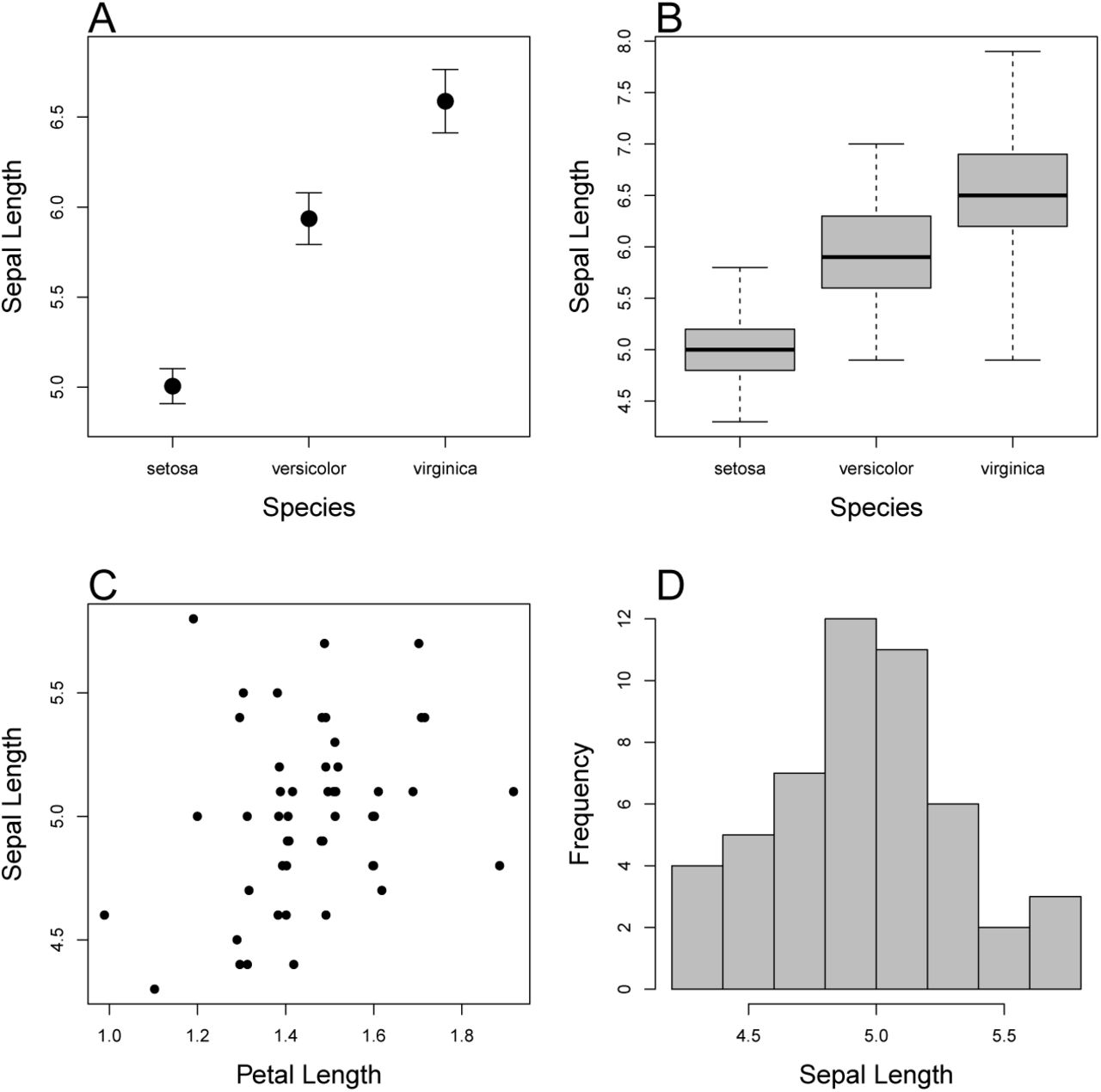
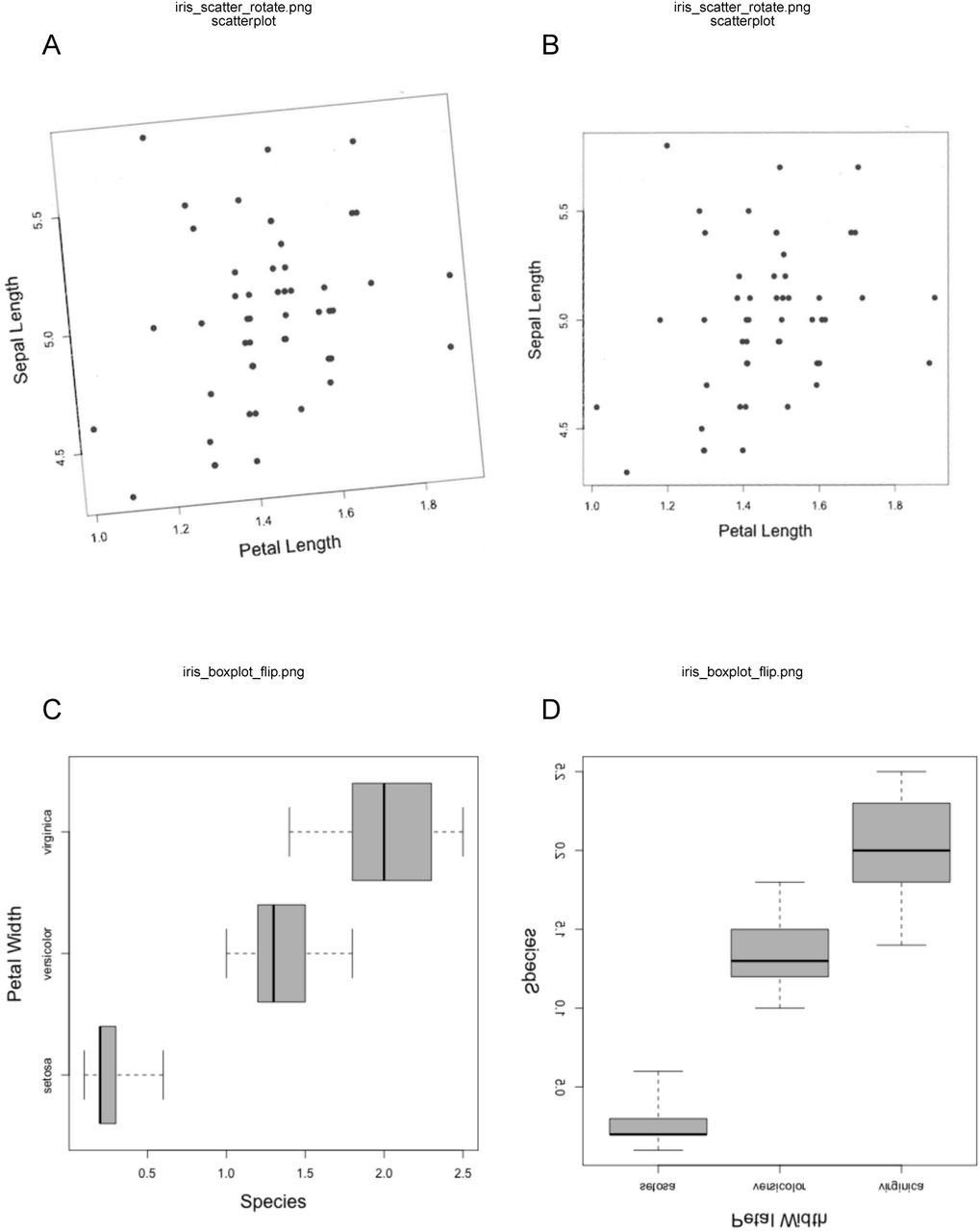
Four plot types that metaDigitise is designed to extract data from: A) mean and error plot, B) box plot, C) scatter plot and D) histogram. Data is taken from the iris dataset in R. A and B are plotted with the whole dataset, C and D are just the data for the species setosa.
Second, digitising programs do not easily allow the integration of metadata at the time of data extraction, such as experimental group or variable names, and sample sizes. This makes the downstream calculations more laborious, as the information has to be added later, in most cases using different software.
Finally, existing programs do not import a set of images and allow the user to systematically work through them. Instead they require the user to manually import images one by one, and export data into individual files, that need to be imported and edited using different software. In essence, existing software does not provide an optimized research pipeline to facilitate data extraction, editing and reproducibility.
These are major issues because extracting from figures can be an incredibly time-consuming process. Furthermore, although meta-analysis is an important tool in consolidating the data from multiple studies, many of the processes involved in data extraction are opaque and difficult to reproduce, making extending studies problematic. Having a tool that facilitates reproducibility in meta-analyses will increase transparency and go a long way to resolving the reproducibility crises we are seeing in many fields (Peng, Dominici & Zeger, 2006; Peng, 2011; Sandve et al., 2013; Parker et al., 2016; Ihle et al., 2017).
Here, we present an interactive R package, metaDigitise, which is designed for large scale data extraction from figures, specifically catering to the the needs of meta-analysts. To this end, we provide tools specific to data extraction from common plot types (mean and error plots, box plots, scatter plots and histograms, see Figure 1). metaDigitise operates within the R environment making data extraction, analysis and export more streamlined. It also provides users with options to conduct the necessary calculations on processed data immediately after extraction so that comparable summary statistics can be obtained quickly. metaDigitise condenses summary data extracted from multiple figures into a single data frame which can be can easily exported. Processed data can also be easily extracted and analysed in any way the user desires in downstream analysis within R. Conveniently, when needing to process many figures at different times metaDigitise will only import figures not already completed within a directory. This makes it easy to add new figures at any time. metaDigitise has also been built for reproducibility in mind. It has functions that allow users to redraw their digitisations on figures, make corrections and access the raw calibration data which is written automatically for each figure that is digitised into a special folder within the directory. This makes sharing figure digitisation and reproducing the work of others simple and easy, and allows meta-analysts to update meta-analyses more easily.
Directory Structure, Image Processing and Reproducibility
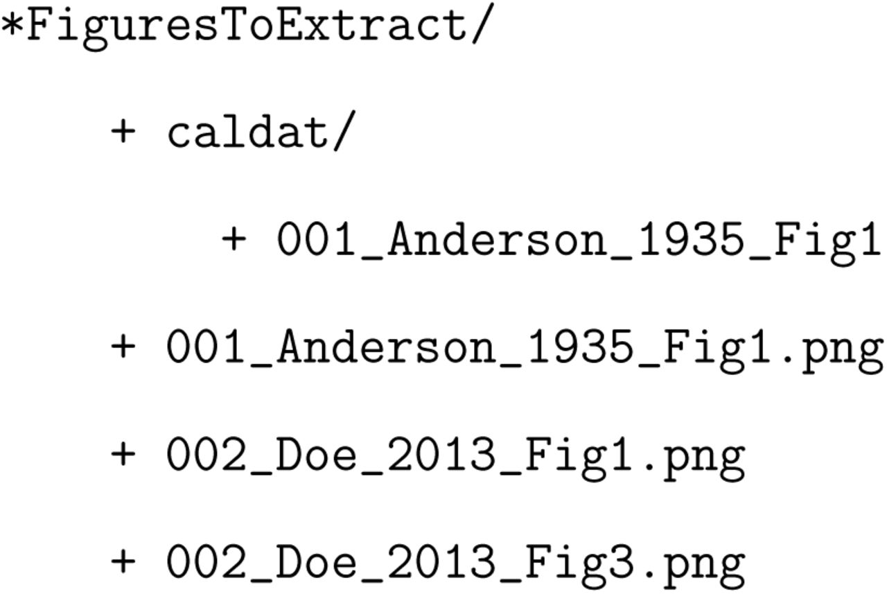
The metaDigitise package is designed to be flexible, yet simple to use. There is one main function in the package, metaDigitise(), which interactively takes the user through the process of extracting data from figures. metaDigitise() was created with the idea that the user would likely have multiple images to extract from. It therefore operates in the same way whether the user has one or multiple images. metaDigitise() is designed to work on a directory containing images of figures copied from primary literature, in .png, .jpg, .tiff, .pdf format. This directory is specified to metaDigitise() through the dir argument. The user is free to set their own broad directory structure (e.g. one directory for all images or one directory for each paper extracted from). We would recommend having all files for one project in a single directory with an informative and unambiguous naming scheme for images to make it easy to identify the paper and figure the data come from. This cuts out the need to change directories constantly. For example the directory structure could look like:

It is important for the user to think about their directory structure early on in this process (also more generally in the context of their entire project), especially if they plan to share the extractions with collaborators or when publishing the project.
When metaDigitise() is run, it recognizes all the images in a directory and automatically imports them one by one, allowing the user to click and enter relevant information about a figure as they go. This expedites digitising figures by preventing users from having to constantly change directories and / or open new images. The data from a completed image is automatically saved as a metaDigitise object in an .RDS file to a caldat directory that is created within the parent directory when first executing the metaDigitise() function. These files enable re-plotting and editing of images at a later point (see below).
A particularly powerful and flexible aspect of metaDigitise() is its ability to identify images that have been previously digitised and only import images that have not been digitised in subsequent calls of the function. This means that all figures do not need to be extracted at one time and that new figures can be added as the project develops. After each image is extracted, the user is asked whether they wish to continue or quit the extraction process. Upon rerunning metaDigitise(), previously digitised figures are simply ignored during processing, but their data is re-integrated within the final output after new files are completed automatically.
After completing all images, or upon quitting, the processed data (in a form specified by the user) is then returned. From all plot types, metaDigitise() summarises the data from a figure as a mean, standard deviation and sample size, for each identified group within the plot (should multiple groups exist). These are the descriptive statistics needed to create many of the relevant effect sizes and sampling error for a meta-analysis. In the case of scatter plots, metaDigitise() also returns the correlation coefficient between the points within each identified group.
Diverse Plot Types
metaDigitise recognises four main types of plot; Mean and error plots, box plots, scatter plots and histograms, shown in Figure 1. Each of these can be processed together and integrated into a single output. Alternatively, users can keep like figures together and process them separately.
In order to correctly extract data from figures metaDigitise() always requires the user to calibrate the axes in the figure. To do this, the user is required to click on two known points on the axis in question, and then enter the value of those points in the figure. Using this information, metaDigitise() then calculates the value of any clicked points in terms of the figure axes. In the case of mean and error plots and box plots, it calibrates only the y-axis (assuming the x-axis is redundant). For scatter plots and histograms both axes are calibrated.
Mean and error plots
metaDigitise() prompts the user to enter group names and allows the user to enter sample sizes (n), which are used in downstream processing. The user is then prompted to click on an error bar followed by the mean. Error bars above or below the mean can be clicked - sometimes one is clearer than the other. metaDigitise() assumes that the error bars are symmetrical. Where the user has clicked the error is displayed in a different colour to the mean (Figure 2A). The user can subsequently add more groups, edit groups or remove groups. Finally the user is asked what type of error was used in the figure: standard deviation (SD, σ), standard error (SE) or 95% confidence intervals (CI95). Standard deviation is calculated from standard error as

and from 95% confidence intervals as

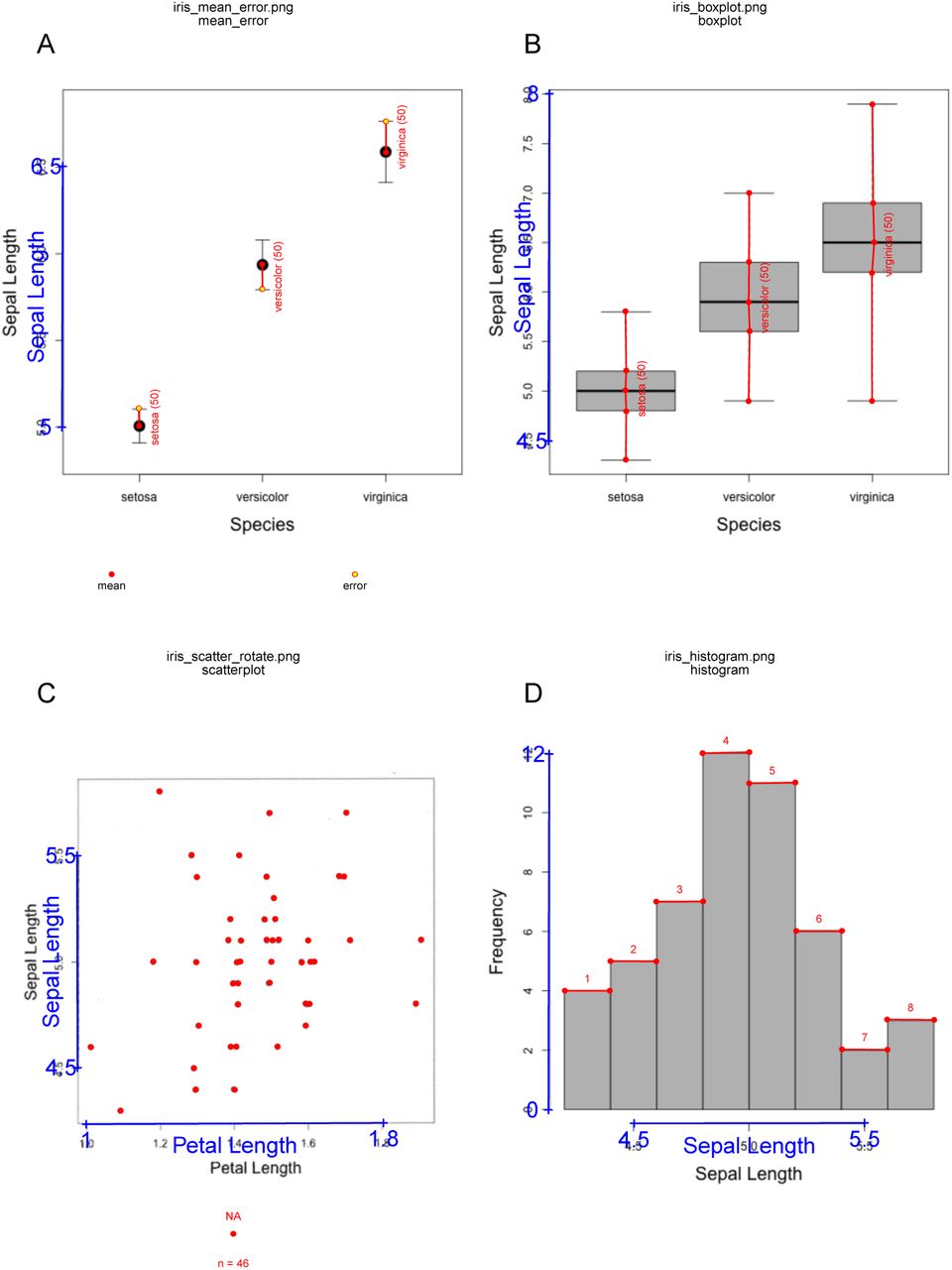
Demonstration of data extraction from different plot types
If the user does not enter a sample size at the time of data extraction (if, for example, the information is not readily available) the SD is not calculated. This can be entered at a later time, however (see below). A function, error_to_sd(), that converts the different error types to SD is also available in the package.
Box plots
As with mean and error plots, metaDigitise() prompts the user to enter group names and allows the user to enter sample sizes (n), which are used in downstream processing. The user is then prompted to click on the maximum (b), upper quartile (q3), median (m), lower quartile (q1) and minimum (a). metaDigitise() will check that the maximum is greater than the minimum, and return a warning if that is not the case. The user can subsequently add, edit or remove groups. From the extracted data, the mean (μ) and SD are calculated as

following Bland (2015) and

where Φ-1(z) is the upper zth percentile of the standard normal distribution, following Wan et al. (2014). As with mean and error plots, if the user does not enter a sample size at the time of data extraction the SD is not calculated. Two functions, rqm_to_mean() and rqm_to_sd(), that convert box plot data to mean and SD respectively are also available in the package.
Scatter plots
metaDigitise() prompts the user to enter groups names and then to click on points. Points added by mistake can be deleted. The user can subsequently add groups, edit groups (add or remove points) or delete groups. Different groups are plotted in different colours and shapes, with a legend at the bottom of the figure (Figure 2C). Mean, SD and sample size are calculated from the clicked points, for each group. Where the sample size from the clicked points does not match a known sample size (e.g. if there are overlaid points), the user can enter an alternate sample size.
Histograms
metaDigitise() prompts the user to click on the top corners of each bar. Bars can subsequently be deleted. For each bar a midpoint (m; mean x coordinates) and a frequency (f; mean y coordinates, rounded to the nearest integer) is calculated. The sample size, mean and SD are calculated as:


As with the scatterplots, if the sample size from the extracted data does not match a known sample size, the user can enter an alternate sample size.
Extracting Data From Plots
We will now demonstrate how metaDigitise() works using figures generated from the well known iris data set. Users can install the metaDigitise package from GitHub as follows:
R> install.packages("devtools") R> devtools∷install_github("daniel1noble/metaDigitise") R> library(metaDigitise)Assume that the user would like to extract descriptive statistics from studies measuring sepal length or width in iris species for a fictitious project. There are a few studies that only present these data in figures. As the user reads papers found from a systematic search, they add figures with relevant data to a “FiguresToExtract” folder as follows
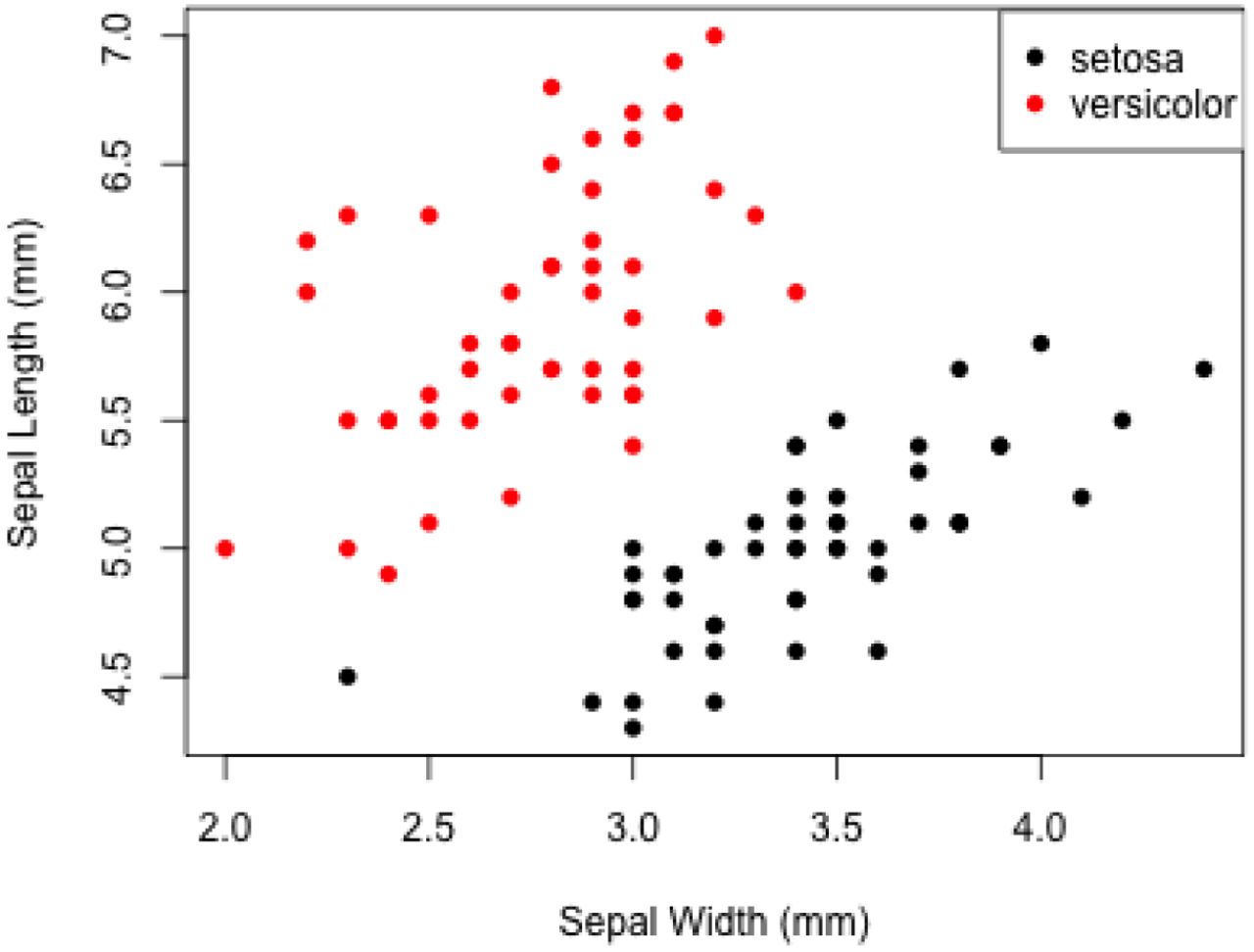
*FiguresToExtract/ + 001_Anderson_1935_Fig1.pngHere, the naming of the files placed in the folder will contain the paper number, first author and the figure number to keep data uniquely associated with figures. At first there is one figure in the folder, shown in Figure 3. Running metaDigitise() brings up a series of prompts for the user using a main menu that provides access to a number of its features (”…” here represents the user’s path to the project directory):
R> digitised_data <- metaDigitise(”…/FiguresToExtract”, summary = TRUE) Do you want to… 1: Process new images 2: Import existing data 3: Edit existing data Selection:
Example scatterplot (001_Anderson_1935_Fig1.png) of sepal length and width for two species of iris (setosa and versicolor)
The user simply enters in the numeric value that corresponds to what they would like to do. In this case they want to “Process new images”. The user is then asked whether there are different types of plot(s) in the folder. This question is most relevant when there are lots of different figures in the folder because it will then ask the user for the type of figure as they are cycled through.
Are all plot types Different or the Same? (d/s)metaDigitise() then asks the user whether the figure needs to be rotated or flipped. This can be needed when box plots and mean and error plots are not orientated correctly. In some cases, older papers can give slightly off angled images which can be corrected by rotating. So, in this prompt the user has three options: f for “Flip”, r for “rotate” or c for “continue”.

After this, metaDigitise() will ask the user to specify the plot type. Depending on the figure, the user can specify that it is a figure containing the mean and error (m), a box plot (b), a scatter plot (s) or a histogram (h). If the user has specified d instead of s in response to the question about whether the plot types are the same or different, this question will pop up for each plot, but will only be asked once if plots are all the same.
Please specify the plot_type as either: m: Mean and error b: Box plot s: Scatter plot h: Histogram R> sAfter selecting the figure type a new set of prompts will come up that will ask the user first what the y and x-axis variables are. This is useful as users can keep track of the different variables across figures and papers. Here, the user can just add this information in to the R console. Once complete, details on how to calibrate the x and y-axis appear, so that the relevant statistics / data can be correctly calculated. When working with a plot of mean and standard errors, the x-axis is rather useless in terms of calibration so metaDigitise() just asks the user to calibrate the y-axis.

The user can just follow the instructions on screen step-by-step (instructions above have been truncated by ‘…’ to simplify), and in the order specified. Before moving on, the user is forced to check whether or not the calibration has been set up correctly. If n is chosen because something needs to be fixed then the user can re-calibrate.
What is the value of y1 ? R> 4.5 What is the value of y2 ? R> 7 What is the value of x1 ? R> 2 What is the value of x2 ? R> 4 Re-calibrate? (y/n) R> nOften, plots might contain multiple groups that the meta-analyst wants to extract from. metaDigitise() handles this nicely by prompting the user to enter the group first, followed by digitisation of this groups data. After digitising the first group, and having exited, metaDigitise() will ask the user whether they would like to add another group. Users can continually add groups (a), delete groups (d), edit groups (e) or finish a plot and continue to the next one (f - if another plot exists). The number of groups are not really limited and users can just keep adding in groups to accommodate the different numbers that may be presented across figures (although it can get complicated with too many).
If there are multiple groups, enter unique group identifiers (otherwise press enter) Group identifier: R> setosa Click on points you want to add. If you want to remove a point, or are finished with a group, exit by clicking on red box in bottom left corner, then follow promptsTo finish selecting points, the user can exit by clicking on the red button that appears when extracting points. The user is then asked if they want to add or delete points from that group.
Add or Delete points to this group, or Continue? (a/d/c) R> cOnce we are done digitising all the groups our plot will look something like Figure 4.
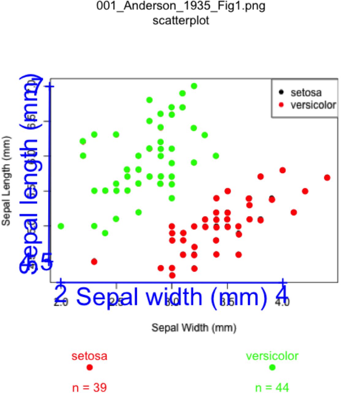
Digitisation of sepal length and width for two species of iris (setosa and versicolor). Names of the variables and calibration (in blue) are plotted alongside the digitised points (green = versicolor; red = setosa). The sample sizes for each group are provided on the lower part of the plot. All figures are clearly labelled at the top to remind users of the filename and plot type. This reduces errors throughout the digitisation process.
When completed metaDigitise() will write the digitised data as a metaDigitise object to a RDS file in the caldat directory, such that our new directory structure is as follows

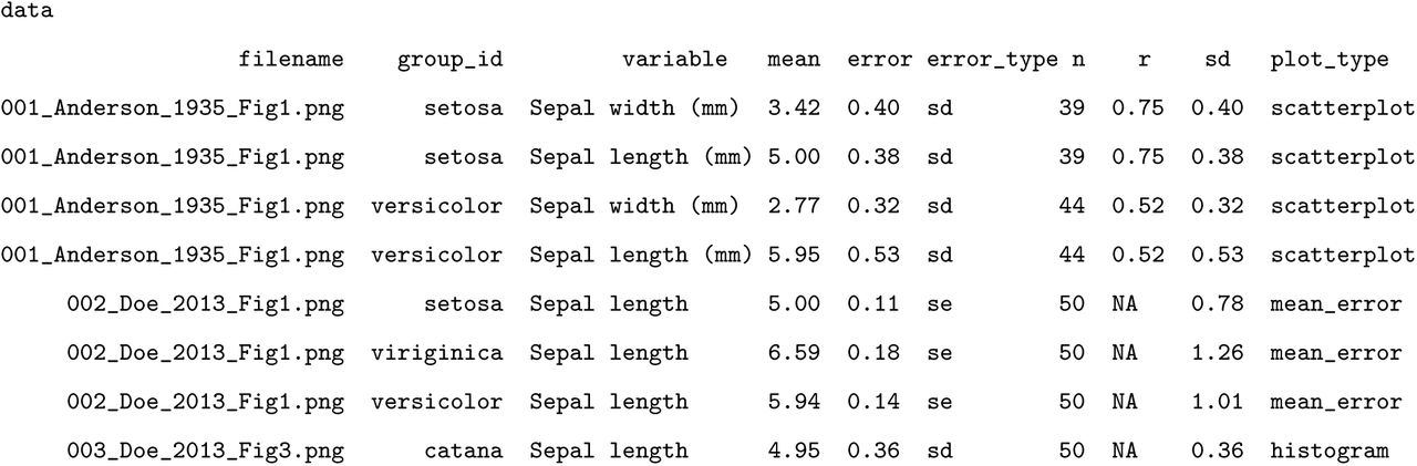
Users can access the metaDigitise object created (001_Anderson_1935_Fig1) at any time using the metaDigitse() function. In the R console, the summarised data for the digitised figure can be printed on screen or even written to a .csv file:
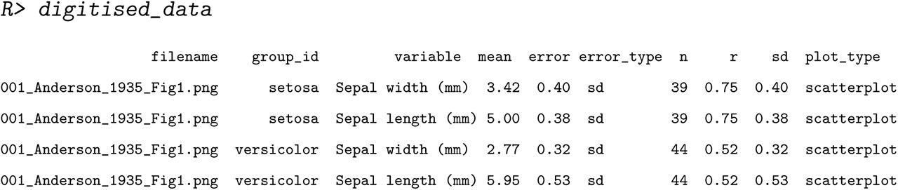
The mean for each of the two variables, along with the two species, are provided. Since this is a scatterplot, the user also gets the Person’s correlation coefficient between sepal length and width for each species. These match reasonably well with the actual means of sepal length and width for each of the species in the full ‘iris’ dataset:

One thing anyone with a familiarity with the iris dataset will notice is that the sample sizes for each of these species (which are n = 50 each) are quite a bit lower. This is an example of some of the challenges when extracting data from scatter plots. Often data points will overlap with each other making it impossible (without having the real data) to know whether this is a problem. However, a meta-analyst will probably realise that the sample sizes here conflict with what is reported in the paper. Hence, metaDigitise also provides the user with options to input the sample sizes directly (see Editing section below), even for scatter plots and histograms where, strictly speaking, this should not be necessary.
Nonetheless, it is important to recognise the impact that overlapping points can have on summary statistics, particularly its effects on standard deviation (SD) and standard error (SE). Here, the mean point estimates are nearly exactly the same as the true values, but the SD’s are slightly over-estimated:

Adding new figures
Users can add additional figures as new papers with relevant information are found. Each figure should be in its own file with unique naming, even if a single paper has multiple figures for extraction. For example, another paper on different populations (and one new species) of iris contained two additional figures where important data could be extracted. These figures can simply be named accordingly and added directly to the same extraction folder:

The user has already processed one figure (001_Anderson_1935_Fig1.png). We can tell this because the caldat folder has digitised data in it (caldat/001_Anderson_1935_Fig1). Now the user has two new figures that have not yet been digitised. This example will nicely demonstrate how users can easily pick up from where they left off and how all previous data gets re-integrated. It will also demonstrate how different plot types are handled. All we have to do to begin, is again, provide the directory where all the figures are located:
R> digitised_data <- metaDigitise("…/FiguresToExtract", summary = TRUE)The user gets the same set of prompts and simply chooses option one. This will permit users to digitise new figures, and will integrate previously completed digitisations along with newly digitised data together at the end of the session, or when the user decides to quit. This time, 001_Anderson_1935_Fig1.png is ignored and the new plots cycle on screen; first 002_Doe_2013_Fig1.png and then 002_Doe_2013_Fig3.png. Since there are a few different figure types, the user answers the first question in the R console as “d”:

Here, the user specifies the new plot type as m for 002_Doe 2013_Fig1.png because the user has a plot of the mean and error of sepal length for each of the three species. The user is then prompted a bit differently from our scatter plot as the x-axis is not needed for calibration:

Again, metaDigitise() will simply guide the user through digitising each of these figures describing to them exactly what needs to be done. At any point if mistakes are made the user can choose relevant options to edit or correct things before ending the figure. This process continues for each plot so long as the user would like to continue and after completing a single plot the user is always prompted as follows:
Do you want continue: 1 plots out of 2 plots remaining (y/n) R> yThis continues until users have completed all non-digitised figures in the folder, at which point metaDigitise() concatenates the new data with previously digitised data in the object:
Re-importing, Editing and Plotting Previously Digitised data
A particularly useful feature of metaDigitise is its ability to re-import, edit and re-plot previously digitised figures. We can do this from the initial options from metaDigitise()
R> digitised_data <- metaDigitise("…/FiguresToExtract") Do you want to… 1: Process new images 2: Import existing data 3: Edit existing data Selection:If the user chooses “Import existing data”, they have the option of either 1) importing data from all digitised images or 2) importing data from a single image that has been digitised. If 2, then a list of files are provided to the user that they can select. Editing existing data allows users to easily re-plot or edit information or digitisations that have previously be done for any plot. This is accomplished by guiding the user through a new set of options:
Choose how you want to edit files: 1: Cycle through images 2: Choose specific file to edit 3: Enter previously omitted sample sizes Selection:If the user is unsure about the name of the specific figure they need to edit or simply want to just check the digitisations of figures they can choose “Cycle through images”, which will bring up each figure, one by one, overlaying the calibrations, group names (if they exist), sample sizes (if they were entered) and the selected points. The user will then be given the choice to edit individual images. Alternatively, choosing option 2, will bring up a list of the completed files in the folder and the specific file can be chosen, at which point it will be replotted. Either of these options will cycle through a number of questions asking the user what they would like to edit:
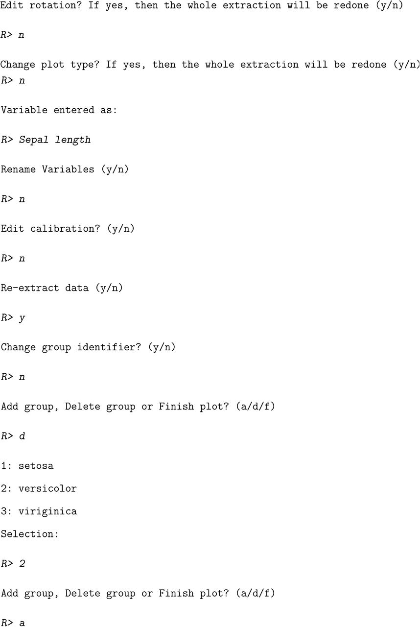
A whole host of information can be edited including the rotation, plot type, the variable name(s) that were provided, the calibration and even the digitisation of groups. When editing the metaDigitise object is re-written to the caldat folder and the edits are immediately integrated into the existing object once complete.
Additional Features
Figure Rotation and Adjustment
Figures may have been extracted from old publications, for example from scanned images, and so are not perfectly orientated on the image. This will make the calibration of the points in the figure from the image problematic. metaDigitise() allows users to rotate the image. By clicking two points on the x-axis, metaDigitse calculates the angle needed to rotate the image so the x-axis is horizontal, and rotates it. (Figure 5A,B)

Figure rotation. A) and B) show how non-aligned images can be realigned through user defined rotation. C) and D) show how figures can be reorientated so as to aid data input.
Furthermore, some figures, including mean and error, boxplots or histograms, may be presented with horizontal bars. metaDigitise() assumes that the bars are vertical, but allows the user to flip the image so that the bars are vertical if provided horizontally (Figure 5C,D).
Obtaining Processed Data
While metaDigitise() provides users with the summary statistics by default, for all plot types, in many cases the user may actually be interested in obtaining the processed digitised data from scatter plots (i.e. calibrated points). This is very easy to do my changing the default summary argument from TRUE to FALSE in metaDigitise(). Instead of providing the user with summary statistics it will return a list containing four slots for each of the figure types (mean error, box plot, histogram and scatter plots). An example of a data object returned from digitising figures is as follows:

Here, the user can easily access the list of processed scatter plot data by simply extracting the scatter plot slot:
>R scatterplot <‐ data$scatterplotAdding sample sizes to previous Digitisations
In many cases important information, such as sample sizes, may not be readily available or clear when digitising figures. In these circumstances users will have answered ‘no’ to the question about whether they have sample sizes or not while digitising. To expedite finding and adding in these sample sizes to do the necessary calculations (if for example a figure presented 95% CI’s or standard errors), metaDigitise() has s specific edit option that allows users to enter in previously omitted sample sizes. It works by first identifying the missing sample sizes in the digitised output, re-plotting the relevant figure and then prompting the user to enter the sample sizes for the relevant groups in the figure, one by one. As an example, assume that we were missing sample sizes for two groups in 002_Doe_2013_Fig1.png:
Here, we can see that we are missing the sample sizes for setosa and viriginica, and as a result, sd is not calculated because metaDigitise() needs this information to make the calculation. If the user found this information after contacting the authors for clarification then they can add these back in as follows:
R> digitised_data <- metaDigitise("…/FiguresToExtract") Do you want to… 1: Process new images 2: Import existing data 3: Edit existing data Selection: R> 3 Choose how you want to edit files: 1: Cycle through images 2: Choose specific file to edit 3: Enter previously omitted sample sizes Selection: >R 3metaDigitise() will replot the figure after this and list, only the groups missing data, for which the user can then update the data. This is then re-integrated back into the data automatically and the sd calculated.
Group " setosa ": Enter sample size R> 50 Group " viriginica ": Enter sample size R> 50Inter-observer Variability and Validation
Inter-observer variability in digitisations
In order to evaluate the consistency of digitisation using metaDigitise between users, we simulated a dataset of two traits with two different groups. These data were then used to construct plots of the four different types (scatterplot, mean and error, histogram and boxplots). Each variable was plotted twice for each given plot type (figures were modified slightly to give users a sense that they were digitising new data) generating a total of 14 figures. 15 independent digitisers were provided with a directory with all 14 figures in a randomised order. Digitisers ran metaDigistise on their own computers, across different operating systems (including Mac, Windows and Linux). Digitisers varied in their level of experience, from people with experience of meta-analyses or comparative work to those without any science background. We asked users to digitise all 14 figures and collected the mean, standard deviation and correlation coefficient (for scatterplots) generated by metaDigitise() for every plot digitised. We transformed these data to standardized differences as

Where θ is the estimate value and  is the true value, meaning that deviations were percentage differences from the true summary statistics. The correlation coefficient deviation was not divided by the true value, as it is already on a standardised scale. This deviation can be seen as a measure of bias. The resulting data was used to assess between- and within- user variability (i.e., the intra-class correlation coefficient) in the data. This was done using linear mixed effect models with user identify as a random effect. Standardised mean, standard deviation and correlation coefficients were used as response variables in seperate models. Sampling variance for ICC estiamtes was generated based on 1000 parametric bootstraps of the model and the significance was tested using liklihood ratio tests. These models were run using the lme4 (Bates et al., 2015) and rptR (Stoffel, Nakagawa & Schielzeth, 2017) packages in R.
If digitisations were consistent across all users then we should find no significant between user variability in the data. Indeed, across plot types we found no evidence for any inter-observer variability in digitisations for the mean (ICC = 0, 95% CI = 0 to 0.029, p = 1), standard deviation (ICC = 0, 95% CI = 0 to 0.033, p = 0.5) or correlation coefficient (ICC = 0.053, 95% CI = 0 to 0.296, p = 0.377). There were was little bias between digitised and true values, on average 1.63% (mean = 0.02%, SD = 4.9%, r = -0.03%) and overall there were only small absolute differences between digitised and true values, deviating, on average 2.18% (mean = 0.40%, SD = 5.81%, r = 0.33%) across all three summary statistics.
SD estimates from digitisations are clearly more prone to error than means or correlation coefficients. If the mean absoluate difference is calculated for each plot type, we can see that this effect is driven mainly by extraction from boxplots and histgrams (% difference):

This is because SD estimation from the summary statistics extracted from boxplots is more error prone, especially at small sample sizes (Wan et al., 2014).
Testing the accuracy of digitisations
To test how accurate metaDigitise is at matching points to their true values, we generated four random scatterplots, each with 20 data points, and digitised these with metaDigitise(). This was done by one digitiser, as there is no detectable between user variation. Data digitised using metaDigitise was essentially perfectly correlated with the true simulated data for both the x-variable (Pearson’s correlation; r = 0.9999915, t = 2137.4, df = 78, p < 0.001) and y-variable (r = 0.9999892, t = 1897.8, df = 78, p ¡ 0.001).
Discussion and Conclusions
Although metaDigitise is already very flexible, and provides functionality not seen in any other package (Table 1) it is clear that there are some functions that it does not perform. A notable feature that metaDigitise lacks is automated point detection. Point detection is available in several packages (Table 1). However, from our experience of using these functions, manual digitising is more reliable and often equally as fast. Particularly given that calibration (for point detection) needs to be done for each plot individually in any case. Additionally, auto-detection often misses many points which then subsequently need to be manually added. Based on tests of metaDigitise (see above), figures can be extracted in around 1-2 minutes, including the entry of metadata. As a result, we do not belive that current automated point detection provides substantial benefits in terms of time or accuracy.
Another feature that metaDigitise (currently) lacks, is an ability to zoom in on plots. Zooming may enable users to gain greater accuracy when clicking on points. However, from our own experience (and indeed from the results above), if you are using a reasonably sized screen then the accuracy is already high from these programs, and there is not much gain to be had from zooming in on points in many circumstances.
In contrast to some other packages, metaDigitise currently also does not extract lines from figures. In our own experience, line extraction is not particularly useful for meta-analysis, although we recognise that it may be useful in other fields. Should a user like to extract lines with metaDigitise, we would recommend extracting data as a scatter plot, and clicking along the line in question. A model can then be fitted to these points (setting the argument “summary = FALSE” in metaDigitise - will provide access to the processed data) to estimate the parameters needed.
Comparison of functionality between different digitisation softwares.
Finally, metaDigitise currently does not allow for asymmetric error bars. At present this is a deliberate omission, as it is not clear how best to derive SD from such data, given also that such asymmetric error bars may represent different things in different figures.
Descriptve statistics are usually the most robust sources of information for calculating effect size statistics (Noble et al., 2017). These are most often presented in figures. Users may therefore also want to compare effect size estimates from inferential statistics with those derived from descriptive statistics (obtained for example using metaDigitise) from a paper. Comparing these different effects sizes can be useful in identifying uncertainties and problems within a paper. In the future, we hope to provide functions to easily convert inferential statistics to standardised effect size estimates, which can seamlessly be integrated with summary statistics from metaDigitise, to calculate equivalent standardised effect size estimates and their sampling variance.
Increasing the reproducibility of figure extraction for meta-analysis and making this laborious process more streamlined, flexible and integrated with existing statistical software will go a long way in facilitating the production of high quality meta-analytic studies that can be updated in the future. We belive that metaDigitise will improve this research synthesis pipeline, and will hopefully become an integral package that can be added to the meta-analysts toolkit.
Acknowledgments
We thank the I-DEEL group at UNSW for incredibly useful feedback, and a host of colleagues for testing, providing feedback and digitising including: Rose O’Dea, Fonti Kar, Malgorzata Lagisz, Julia Riley, Diego Barneche, Erin Macartney, Ivan Beltran, Gihan Samarasinghe, Dax Kellie, Jonathan Noble, Yian Noble and Alison Pick. JLP was supported by a Swiss National Science Foundation Early Mobility grant (P2ZHP3_164962), DWAN was supported by an Australian Research Council Discovery Early Career Research Award (DE150101774) and UNSW Vice Chancellors Fellowship and SN an Australian Research Council Future Fellowship (FT130100268).


