

Abstract
There is increasing interest in developing diagnostics that discriminate individual mutagenic mechanisms in a range of applications that include identifying population specific mutagenesis and resolving distinct mutation signatures in cancer samples. Analyses for these applications assume that mutagenic mechanisms have a unique relationship with neighboring bases that allows them to be distinguished. Direct support for this assumption is limited to a small number of simple cases, e.g. CpG hypermutability. We have directly evaluated whether the mechanistic origin of a point mutation can be resolved using only sequence context for a more complicated case. We contrasted mutations originating from the multitude of mutagenic processes that normally operate in the mouse germline with those induced by the potent mutagen N-ethyl-N-nitrosourea (ENU). The considerable overlap in the mutation spectra of these two samples make this a challenging problem. Employing a new, robust log-linear modelling method, we demonstrate that neighboring bases contain information regarding point mutation direction that differs between the ENU-induced and spontaneous mutation classes. A logistic regression classifier proved to be substantially more powerful at discriminating between the different mutation classes than alternatives. Concordance between the feature set of the best classifier and information content analyses suggest our results can be generalized to other mutation classification problems. We conclude that machine learning can be used to build a practical classification tool to identify the mutation mechanism for individual genetic variants. Software implementing our approach is freely available under the BSD 3-clause license.
Author Summary Mutations are a fundamental contributor to developing diversity in biological capabilities. There are a multitude of processes that affect how DNA is damaged and whether the damage is repaired in such a way as to produce a mutation. In some instances, mutation is a key adaptive feature of normal biological tissue development. For instance, some immune cells employ enzymatic machinery to elevate the mutation rate to generate additional diversity in the molecules responsible for recognizing pathogens. Mutation is also key to abnormal developmental processes, such as those characterizing cancers. For these and other applications, knowing the mechanisms by which individual mutations arise would enhance our understanding of the biology. Here, we have established and exploited the existence of a relationship between the DNA sequence immediately flanking point mutations and the mechanism of mutation. Using machine learning techniques, we demonstrate how to distinguish mutations that occurred by normal cellular processes from those induced by a potent mutagen. The resulting classifiers showed very strong performance in a manner that was robust. Our results demonstrate the potential for high resolution determination across the genome of where individual mutagenesis mechanisms have operated.
Introduction
In most catalogs of genetic variation, the data consist of variants that derive from a mixture of mutagenic processes. Whether analysis of the genetic variants alone allows resolving the causative mechanism for an individual genetic variant remains an open question. Instances of a singular etiological relationship between point mutation mechanism and flanking sequence are known for only a small number of relatively simple cases. From a biochemical perspective, it seems a reasonable conjecture that the sequence of neighboring bases should affect mutagenic processes in general. This conjecture remains substantively unverified as is the related conjecture that knowledge of neighbouring sequence is sufficient to identify the specific mutagenic origin. Methods have been developed that can discriminate between entire mutation spectra (Zhu et al., 2017), such as those characteristic of cancers, and to estimate the major components of these spectra (Alexandrov et al., 2013; Shiraishi et al., 2015). As far as we are aware there has not been a detailed examination of the relationship between a mutation mechanism and neighbouring bases with a view to identifying mechanistic origins of individual variants. Here, we employ machine learning methods to address this using a data set of point mutations of known origin. We limit discussion, and analysis, to the 12 distinct single nucleotide point mutations.
In mammals, mutation processes exhibit considerable heterogeneity which manifests between genomic locations, cell types, disease states and clinical treatments. The within-genome heterogeneity of sequence composition is taken as an indicator of the heterogeneous operation of mutation processes operating in the germline and multiple factors are implicated in driving this pattern (Hodgkinson and Eyre-Walker, 2011). These include factors that distinguish gametogenesis between the sexes (e.g. Huttley et al., 2000), which manifest at the level of entire chromosomes, to the localized operation of transcription-coupled DNA repair processes (e.g. Svejstrup, 2002). There is also considerable complexity in the origin of mutations affecting somatic tissues. Variation in mutagenesis distinguishes normal cell lineages, as evidenced by the biochemically specified somatic hypermutation that occurs in immune cells (Chahwan et al., 2012). The spectrum of mutations can be a distinctive feature of different cancers (Pleasance et al., 2010). This may result from tissue-specific exposure to exogenous mutagens, such as the reported excess of G → T* transversions (where * indicates a mutation direction and its strand complement) in smoking-associated lung cancer (Hainaut and Pfeifer, 2001). It may also reflect defects in specific DNA repair processes (Viel et al., 2017). In all of these cases the catalog of mutations arises from a mixture of different processes, making assignment of a specific cause to a single mutation challenging.
Germline heterogeneity in mutagenesis has been correlated with a number of genomic features and processes including the abundance of G and C nucleotides (hereafter GC) and sexual dimorphism in gametogenesis. The primary explanation for the positive correlation with GC is that it reflects a causal relationship with the recombination rate via the process of biased gene conversion (Hellmann et al., 2005; Hodgkinson and Eyre-Walker, 2011; Meunier and Duret, 2004). Differences between the sexes in the spectrum of point mutations leads to differences in GC between chromosomes based on time spent in the male germline (Huttley et al., 2000).
We can decompose the process of a mutation into two fundamental steps: lesion formation followed by a failure of DNA repair to reconstitute the original base pair. High exposure of cells to UV light, which elevates formation of dipyrimidine lesions, illustrates the role of lesion creation on mutagenesis (Pfeifer et al., 2005). The accumulation of defects in DNA mismatch repair genes, which contribute to development of colorectal cancer, illustrate the role of defective DNA repair (Viel et al., 2017). In both of these cases, the rate at which the different point mutations occur can be affected, highlighting that different types of point mutation can have a common mechanistic origin. As systemic changes to mutation process are a feature of cancer cells, a primary analysis focus in cancer biology has to been to resolve mutagenic signatures that characterize cancers (Alexandrov et al., 2013; Shiraishi et al., 2015). This work exploits the presumed relationship between point mutation processes and flanking DNA sequence.
The nucleotides flanking a mutated position contain information regarding the mutagenesis process responsible for the change. Hypermutability of the CpG dinucleotide illustrates the relationship between neighbouring bases and point mutation mechanism. Association of a 3’-G with elevated C→T mutation rates derives from the binding preference of DNA methylases (Krawczak et al., 1998). These enzymes bind to this dinucleotide and modify C to 5-methyl-cytosine. The resulting modified base exhibits a 10-fold increase in spontaneous deamination rate, an effect so pronounced as to almost entirely swamp alternate causes of C→T mutations (Zhu et al., 2017). The apparent simplicity of the relationship between C→T point mutations and flanking nucleotides reflects the dominance of a single chemical process in creating lesions.
The sequence motifs associated with non-C→T point mutations are more complicated (Zhu et al., 2017), suggesting contributions from multiple mutagenesis mechanisms. It was shown from an analysis of millions of human germline mutations that more than one nucleotide at flanking positions were associated with the non-C→T point mutations (Zhu et al., 2017). This is consistent with multiple mutation mechanisms contributing to these point mutations. At present, the mechanistic basis underlying these mutation associated sequence motifs (mutation motifs) remains unknown. Even in the case of cancer, the diversity of defects in DNA repair that afflict these cells limit our certainty regarding the possible mechanisms that may be responsible for a specific genetic variant.
The systematic use of mutagens in forward genetic screens provides an opportunity to develop an understanding of the relationship between neighbouring sequence and mutagenesis. N-ethyl-N-nitrosourea (ENU) is a synthetic alkylating chemical widely employed in mutagenesis studies (Álvarez et al., 2003; Lee et al., 2012; Stottmann and Beier, 2014), causing new germline mutations at ~100 times higher rate than the spontaneous mutation rate (Stottmann and Beier, 2014). Exposure to ENU can induce formation of a number of alkylation adducts including N1-adenine (e1A), O4-thymine (e4T), O2-thymine (e2T), and O2-cytosine (e2C)(Noveroske et al., 2000; Shrivastav et al., 2010). If the DNA repair system fails in repairing these adducts, they are mispaired during DNA replication to a non-complementary nucleotide, resulting in a single base change mutation (Justice et al., 1999; Noveroske et al., 2000). The resulting ENU-induced mutations are dominated by A → G* mutations and A → T* mutations, with rare reported occurrences of C → G* mutations (Takahasi et al., 2007).
Whether ENU mutagenesis induces mutations randomly with regards to flanking DNA sequence is debated (Barbaric et al., 2007; Bauer et al., 2015). The unique ENU-induced mutation spectra distribution described above has provided the basis for the ENU-induced variant filtering strategy (Andrews et al., 2012). For example, removing any C → G* transversions, leaves only genetic variants likely to be generated by ENU process and thus candidates for novel phenotypes. We refer to this filtering strategy as the naïve (classification) method, in which the mutation mechanism is assigned solely on the basis of mutation direction. The approach has high accuracy solely because of the excess of ENU-induced mutations. However, there remains a possibility of misclassification of mutation origin in these studies as some fraction of the point mutations labelled as being ENU-induced will instead have originated by non-ENU mutagenesis. If sequence neighborhood does affect mechanism, then mutation classification techniques that exploit this information should improve over the naïve method.
Machine learning techniques are well suited to the problem of sequence-based classification of samples (Ben-Hur et al., 2008; James et al., 2013). The goal of machine learning classification is to find a rule, based on observed object features, that can assign new objects to one of several classes (James et al., 2013; Sonnenburg, 2008). Machine learning techniques have been applied to a diverse array of sequence-based classification problems ranging from microbial taxon assignment (e.g. Bokulich et al., 2018) to predicting the position of nucleosomes in eukaryotic cells from ChIP-seq data (e.g. Peckham et al., 2007).
In this study, we evaluate whether sequence features can improve the performance of classifiers devised to discriminate between mutagen induced and spontaneous point mutations in the mouse germline. We affirmed a highly significant influence of neighboring nucleotides on ENU point mutations and that these associations differ from those evident in spontaneous mutations. Our results reveal that a combination of k-mer size and representation of second-order interactions among nucleotides was able to markedly improve classification performance in comparison to the naïve classifier approach. All scripts developed for this work are made available under an open source license.
Results
Distinctions between ENU-induced and spontaneous point mutations
A logical requirement for using sequence features to discriminate samples is that those features differ in abundance between the samples. We addressed this using two complementary formal hypotheses tests. The “spectra” hypothesis test compares the distribution of point mutation outcomes in the two source materials. The “neighbourhood” hypothesis test contrasts the association of neighbouring bases with those point mutation outcomes. In both cases, ENU-induced germline point mutations were obtained from the Australian Phenomics Facility, and spontaneous germline mutations from Ensembl database (see Materials and Methods).
We employed a log-linear model to test the null of equivalence in mutation spectra between the ENU-induced and spontaneous samples (Zhu et al., 2017). This test considers the relative distribution of outcomes from mutations of, for example, the base T. A separate test was employed for each possible starting base. Consistent with published reports, the spectra of ENU-induced and spontaneous point mutations in the mouse were significantly different (Fig S1 and Table S1). To simplify the following, and as stated in the Introduction, we abbreviate the description of a point mutation and its strand complement using the notation X→Y*, i.e. A→G* refers to both A→G and its strand complement T→C. Direct examination of counts for the ENU-induced mutations reveals they were dominated by A → G* and A → T* mutations, with frequencies of 42% and 27% respectively. These contrast with their abundance in mouse spontaneous mutations of 29% and 3.7% respectively. Visualization of the spectrum analyses (Fig S1) reflects these changes in proportion. These differences affirm the basis for the current naïve mutation classification algorithms applied to ENU samples.
The striking difference in mutation spectra was also accompanied by striking differences in the magnitude and identity of neighbouring base influences. Prior to discussing the results, we briefly describe the log-linear modelling analyses employed. We use position indices that are relative to the point mutation location, defined as position 0, with negative / positive indices representing 5’- / 3’- positions respectively. Consider, for example, the question of whether bases at the position immediately 3’- to a point mutation of A→G associate with the mutation. The test assesses the null hypothesis that in sequences where an A→G mutation occurred, the base counts at the +1 position are equivalent to those at the +1 position for occurrences of A in the reference distribution. This is an example of a single position (first-order), or independent (denoted I in our modelling notation) effect. We can also evaluate whether the joint counts of bases at two positions are equal between the mutated and reference sequence collections (second-order dependence, or 2D). Our previous analyses of spontaneous germline mutations from humans identified neighbour effects as highly influential, and that independent and second-order effects dominated higher-order effects (Zhu et al., 2017). These analyses are readily extended to comparing equivalence between samples, as is the objective here. See Materials and Methods for more details.
Our analyses established there were strongly significant differences between the ENU-induced and spontaneous mutations in the identity of the associated mutation motifs, and their relative magnitude. To simplify the exposition, we limit our discussion here to description of the results from the A→G* case, the most abundant ENU-induced point mutation. (We note that all point mutations exhibited strongly significant differences and summarize these in Table S2). The maximum relative entropy (RE) association of independent positions with A→G was 5-fold larger in the ENU-induced sample. This maximum association was at +1 in the ENU-induced sample, compared with −1 for the spontaneous sample (Fig 1). Using the log-linear model, we rejected the null hypothesis of the equivalence between ENU-induced and spontaneous samples for neighbouring base associations with AEG mutations. While these samples revealed highly significant differences for nearly all effects orders (Table 1), the magnitude of difference was greatest for the I and 2D effects (Fig S2). As mentioned above, these patterns held true for all point mutation directions (Table S2).

Neighboring base associations significantly differ between ENU-induced and spontaneous germline A→G mutations. Position is relative to the point mutation at position 0. RE is relative entropy, derived from the deviance of the log-linear model (Zhu et al., 2017). Letter height is proportional to the relative entropy term for that base. Normally oriented (180°-rotated) letters represent bases that are positively (negatively) associated with the point mutation. See Materials and Methods for more details.
Log-linear analysis comparing neighbour associations between mouse germline and ENU-induced A→G mutations. Deviance is from the log-linear model, with df degrees-of-freedom and corresponding p-value obtained from the χ2 distribution. p-values below 0.025 were determined to be significant.
Of further relevance to feature selection for classifier design is the physical limit to these associations. Estimation of the physical limit of association from longer flanking contexts was obtained using relative entropy as per Zhu et al. (2017) (see Fig S3 and Table S3). The ENU-induced sample showed the physical limit mean, median and standard deviation of 3.2bp, 2bp, and 1.7bp respectively. In contrast, the corresponding statistics for spontaneous mutations were 2.9bp, 2.5bp, and 2bp. As a consequence of this variability, we considered a range of different neighborhood sizes in development of the classifiers.
Development of a two-class machine learning classifier
In developing classifiers, we evaluated a collection of algorithms, sample sizes, sequence feature sets, k-mer size and hyperparameter values (see Materials and Methods for details). Classifier development was strictly limited to data from a single mouse chromosome. We arbitrarily chose chromosome 1 given availability of sufficient data (see Table S4). We note here that we present only the Logistic Regression (LR) classifier results in the manuscript as they performed systematically better than naïve Bayes (NB) classifiers. NB results are in supplementary material.
Classifier performance was measured as the area under the receiver operating characteristic curve (AUC) score. For any particular classifier, its performance was measured using the mean and standard error derived from 5 replicate AUC measures obtained from the cross validation analysis. A classifier whose mean AUC score was greater than that of another classifier was taken to be superior, after considering the standard errors.
In the following, we describe the classifier feature sets using a combination of the terms M, I, 2D, FS and GC%. We refer the reader to Materials and Methods for a more detailed description. These terms correspond to the mutation direction (M), the set of contributions from independent flanking positions (I), and the set of contributions arising from 2-way dependence among flanking positions (2D). The fully saturated (FS) model is a model containing M and all possible independent and multi-position interactions. (In the regressions, the exact values for the I and D terms depend on the value of k.) The GC% corresponds to the percentage of G+C nucleotides in flanking DNA sequence.
For LR, we made choices regarding two hyperparameters. ℓ1 regularization was chosen as it prunes out unneeded features by setting their associated weights to 0 (Bühlmann and Van De Geer, 2011). This allowed us to establish which features contribute to the classification. The regularization parameter C controls overfitting by affecting the trade-off between variance and bias of regression parameter estimates. We selected the value of C that returned the best classifier performance on the validation set (see Materials and Methods).
Comparison of training curves resulting from classifier evaluation indicated that M+I+2D provided robust performance. The learning curves show the sensitivity of the classifier performance to training set size, where the latter is the total of both ENU-induced and Spontaneous classes. For the categorical feature sets, we considered four distinct models: M, M+I, M+I+2D and FS. It can be seen from Fig 2 that when training size is > 4, 000 samples, the rate of classifier performance improvement with increasing sample size drops off markedly. For subsequent comparisons, we used classifiers trained on data sets with ~16,000 samples as their standard errors allowed greater resolution between the feature sets. Of the classifiers that only included categorical features, the naïve classifier employed for classifying ENU-induced mutations, M, was the least accurate. Inclusion of individual position features, represented by I, provided a substantial improvement over M. The best performing classifiers, however, included features representing dependence among positions (see Table S5 for detailed statistics). That said, the overlap in standard errors of the  for the M+I+2D and FS models (Fig 2) indicate that inclusion of two-way dependence captured the majority of information contained by the sequence neighbourhood. The value of C that returned maximal performance was consistently 0.1 for all models and all samples that considered higher-order interactions (i.e. 2D and above).

Model M+I+2D was sufficient for classifying mutations. Learning curves from training data are shown for four proposed classification models from 7-mers: M, M+I, M+I+2D and FS. The mean  and standard error were calculated from the 5 chromosome 1 training samples. See the text for an explanation of model notation.
Choosing neighborhood size
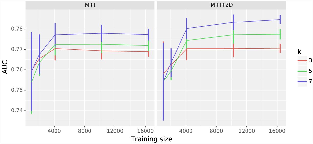
As illustrated by the log-linear analyses reported above, the physical limit of neighboring base influence differs between point mutations and mutation mechanism (Figure S3 and Table S2). We therefore assessed the impact of sequence neighborhood size, comparing performance for three different k-mer sizes (3, 5, 7) for the M+I and M+I+2D feature sets. Comparison of learning curves established that for training set sizes > 4k, classifiers based on a 7-mer context performed better than the other two values of k (Fig 3). The impact of choice of k differed between the feature sets, with the strongest improvements with increasing k evident for the M+I+2D model. In the following analysis, all classification experiments are performed with the 7-mer neighborhood context. (For detailed AUC statistics please refer to Tables S6, S7, and S5.)

Classifier learning curves identified 7-mers as having the best performance. The influence of k-mer choice on learning curves is shown for models M+I and M+I+2D. Plot titles indicate the model being evaluated.  and the standard error were computed as described in Fig 2.
Incorporating GC% feature did not improve the classification performance
As described in the introduction, the existence of a correlation between sequence GC% and mutation processes in mammals has been known for some time. We therefore considered whether inclusion of GC% as a feature would improve classifier performance. GC% was estimated from ±500bp flanking each mutation. Only the naïve classifier (M) performance was improved by inclusion of the GC% feature (Fig S4). The impact on classifiers containing sequence features ranged from no effect (M+I) to substantially worse (FS). We speculate that the improvement of M+GC% over the M feature set arises because the GC% term indirectly measures the base composition of the immediate neighborhood captured by the I term.
Applying classifier to whole genome
From the classifier development process described above, we selected the LR classifier with k = 7, M+I+2D feature set, and hyperparameters ℓ1, C = 0.1 trained on the ~ 16, 000 data sample from chromosome 1. We applied this classifier to all mouse point mutations and display the results by chromosome in Fig 4. The vertical axis is the AUC score for all chromosomes except chromosome 1 where, because it was used for training, it is the average AUC across the 5 different cross-validation samples (see Materials and Methods). With a mean and standard deviation of the chromosome AUC scores of 0.8 and 0.01 respectively, the LR M+I+2D classifier has a relatively good performance across the entire genome. Interestingly, the classifier performed worst with chromosome 1 data.

Per chromosome classification performance on the mouse genome of the LR M+I+2D classifier. The classifier was trained on ~16,000 mutations from chromosome 1. The AUC score obtained after applying the trained classifier to the remaining mutations (not used for training) from the chromosome 1 is represented by the blue bar.
Performance of the one-class classifier was substantially worse
We sought to evaluate whether the mutation motifs associated with spontaneous mutations were sufficiently distinctive as to allow a machine learning algorithm to effectively identify non-spontaneous mutations. This corresponds to an outlier analysis. We tackled this using a one-class (OC) Support Vector Machine (SVM). (See Materials and Methods for more detail.) We considered the same feature set choices as for the LR models in a 7-mer context. As shown in Fig 5, the M+I+2D feature set showed the best performance. However, all OC classifiers had much lower  than even the simplest two-class classifier (M). Furthermore, the OC M+I+2D classifier applied to the entire genome exhibited a systematically lower AUC compared to the LR classifier (Fig 6).

The one-class SVM classifier performed worse than all logistic regression classifiers. x-axis is the size of the training sample, y-axis is the  and standard error were calculated as per Fig 2.

The one-class classifier performs worse than the logistic regression classifier on the entire genome. LR – logistic regression, and OC – one-class Support Vector Machine classifiers. The classifiers were developed on 7-mers with the M+I+2D feature set.
Discussion
We have sought to establish the extent to which the etiological relationship between flanking sequence and mutagenesis can be used to identify the mechanism via which individual point mutations originate. Genetic variants in the mouse arising from application of ENU, a potent chemical mutagen, were contrasted with those arising spontaneously. We show that ENU-induced point mutations are very strongly associated with neighboring bases in a manner that differs to their spontaneous counterparts. A two-class classifier performed markedly better to the current standard technique for identifying ENU mutations and was robust to genomic sequence attributes that have previously been shown to affect mutation processes. Our examination of the potential for machine learning based on the single category of spontaneous germline mutations revealed substantial challenges remain to resolving this more general case.
Comparison of the mutation spectra between spontaneous and ENU-induced germline mutations supported previous conclusions. The spectral analysis compared the breakdown of mutations from a single base mutation from ENU-induced and spontaneous mutations. The proportions of A→G* and A→T* mutations were substantially increased ~1.5 fold and ~7.5 fold, respectively, in the ENU-induced compared to spontaneous sample. These observations are consistent with previous reports (Barbaric et al., 2007; Justice et al., 1999; Noveroske et al., 2000; Takahasi et al., 2007). The abundance of A→G* point mutations in both the ENU-induced and spontaneous samples underscores the challenge of using mutation direction alone for classifying mechanistic origin, and the likelihood that such an approach will be error prone.
Our analyses established that the DNA sequence flanking ENU-induced mutations does contain distinctive information. After correcting for multiple hypothesis tests (Holm, 1979), highly significant associations between neighboring bases and point mutations were found for the ENU-induced sample, along with highly significant differences in neighborhood between the ENU-induced and spontaneous mutations. As ENU induces an elevated rate of DNA lesion formation, it seems plausible these differing neighboring base associations reflect that chemistry. Alternately, they may derive from operation of different DNA repair processes to those typically active in the germline (Noveroske et al., 2000; Shrivastav et al., 2010; Takahasi et al., 2007). In addition to the independent neighborhood effects, all ENU-induced mutations were found to be significantly associated with higher-order effects. Similar to what we was observed from humans (Zhu et al., 2017), the higher-order effects on ENU-induced mutations were evident in a manner such that bases at physically contiguous positions showed the largest RE (Fig S2). The latter may reflect the importance of base stacking on helix stability (Yakovchuk et al., 2006)
Our analyses of the influence of sequence neighborhood on ENU-induced point mutations clarify previous reports. Barbaric et al. (2007) found a significant enrichment of base G or base C at one of the two most immediate flanking positions. Their measurement encompassed all 12 mutation types and thus could not resolve whether this was a systemic influence of ENU, or one related to a specific point mutation. Indicating it is the latter, our analyses identified this specific pair of neighboring bases as highly significantly associated with ENU-induced A→G*. Our results contradict the claim, by Bauer et al. (2015), that there were no neighboring base influences. We note that those authors did not formally test this hypothesis.
A succinct LR model was capable of strong performance, even when trained on just a small fraction of the total data. The current standard classifier, model M, represents the baseline performance. M considers only mutation direction and ignores sequence neighborhood entirely. The performance  of the M+I+2D feature set on the trading data from mouse chromosome 1 was ~ 7% better than that of M while the fully saturated (FS) model exhibited comparable performance (Fig 2). This observation indicates that including dependent effects with order > 2 confers little benefit to classification performance. This observation is consistent with the results from our log-linear analysis which showed a small residual deviance after fitting the I+2D model (Fig S2).
The GC% statistic, previously correlated with mutation processes in mammals, was determined to be a crude surrogate of more explicit neighborhood features. GC% is a sequence composition summary statistic. Inclusion of this feature in the classifier only improved the M model. In all other cases it had no effect or reduced classifier performance (Fig S4). This result emphasizes the mechanistic role of individual bases, as reflected by the mutation motifs (Fig 1), rather than a more general property (e.g. the local DNA melting point) of a sequence region.
Application of the developed LR classifier to the whole genome produced a greater performance than what we observed on the training chromosome. We evaluated classifier performance on a per-chromosome basis to facilitate evaluating whether a relationship existed between classifier performance and the distinctive k-mer distributions reported for mammal sex chromosomes (Huttley et al., 2000). The AUC from the combined sex-chromosomes lay within the range of AUC scores from the autosomes, indicating the discriminatory resolution of the classifier was robust to such differences. The observation that both the two-class and one-class classifiers returned their lowest AUC for chromosome 1 data (the part that had not been used for training) is puzzling (Figs 4, 6). The consistency between these very different machine learning algorithms suggest that mouse chromosome 1 presents a particularly challenging case for classification. The basis for this remains unknown.
It is worth noting that our LR classifier is trained using relatively balanced data, that is the number of ENU and germline mutations were comparable in our data set. This design reflects our interest in understanding what sequence factors affect classifier performance, rather than the specific objective of delivering a classifier for studies employing ENU. In such studies, the mutation classes will be highly imbalanced as we expect many more ENU than spontaneous mutations (up to 100-fold excess). This attribute needs a different trade-off between false positive and false negative predictions from the classifier. There are several extensions to this work that may be useful when a practitioner attempts the class imbalanced task. First is to consider using a performance metric that is less sensitive to class imbalance (Davis and Goadrich, 2006). Second is to extend the learning method to manage class imbalance during training, either using re-sampling methods or cost sensitive methods (Haixiang et al., 2017).
A one-class classifier would also provide a means for generic identification of mutations that did not match a designated reference sample. For instance, a forward genetics screen employing ENU where spontaneous mutations are rare. While the outcome of feature selection identified the feature set M+I+2D as the best performing OC classifier, the  from the genome was 0.67. This is significantly better than a random guess, but just ~84% of the two-class classifier performance. This discrepancy in performance likely reflects the overlap between sequence features of the ENU-induced and spontaneous mouse germline mutations. Since the one-class models are trained only on one sample, they are very sensitive to irrelevant neighborhoods compared to the two-class classifiers. In other words, the presence of “noise” makes it difficult to identify neighborhoods that are unique to the positive class. Furthermore, the one-hot encoding (see Materials and Methods) for one-class classification produces a sparse table for the sample size, which can reduce classification performance.
Both the choice of k and the corresponding feature set can improve over the results obtained here. For values of k in {3, 5, 7}, we considered the full set of alternate feature sets, i.e. M, I, and all possible dependent interaction terms. Classifier performance increased with value of k. There was a trade-off between classifier performance and memory usage with choice of k. This precluded extending k for the comprehensive feature set comparison. We did, however, consider the simpler M+I model for much larger values. The results there indicate additional, potentially quite substantial, gains in performance may be attainable. Learning curve analysis of the M+I model for k = 61 returned  (Fig S5). Inclusion of 2D terms was precluded by memory issues. A potential solution to this arises from restricting the D features to those for physically adjacent positions. Our log-linear analyses revealed the strongest information content exists among dependently interacting positions that are physically adjacent with each other and/or the mutating position. Incorporating this into feature selection could significantly improve classifier performance for both the one and two-class classifier problems.
While we also considered NB, the generally poorer performance of this approach (Fig S7) led us to discard it. There have been systematic examinations of differences between LR and NB classifiers (Ng and Jordan, 2002). These differences are due to the different structural assumptions used by the classifiers. LR is a discriminative classifier, and it directly estimates the conditional probability of interest. NB is a generative classifier, estimating both the prior and likelihood before using them to estimate the posterior probability of interest. The design choice of estimating the likelihood makes NB more sensitive to data that violates the Gaussian noise assumption. Therefore when the underlying data does not exhibit Gaussian noise, LR classifiers have lower asymptotic error than NB. In addition, if training sizes are relatively large, then LR performs better than the NB classifiers (Ng and Jordan, 2002).
Our results have established the utility of including a representation of sequence neighborhoods in classifiers for resolving point mutation origins. There remain open questions as to why should large k be so informative, when the analysis of information content of neighboring bases revealed a quite restrictive limit (Fig S3 and Zhu et al., 2017). Perhaps, as speculated previously (Bauer et al., 2015), this reflects broader sequence features correlated with open chromatin status during spermatogenesis. Irrespective of biological mechanism, the marked improvement in classifier performance we were able to achieve is suggestive further improvements are possible.
We have shown that neighboring positions can be used to classify the mechanistic origins of mutations using machine learning techniques. The LR classifier can be expressed in relation to the log-linear models and this relationship allowed us to “dissect” the contribution level between different positions. However, the classifier features used here were mainly designed for two classes. While we used them for the one-class classification as well, and the performance was better than random guessing, the best customization of feature selection for the one-class classifier remains unresolved. We further restricted our effort to considering only neighborhood sizes up to k = 7. This reflected a practical barrier to looking at larger k due to the feature table becoming too large, and requiring too much memory. Introducing a kernel to the classifier design may be a potential solution to examine a much bigger k in a computationally efficient way. Kernel functions can be developed to examine the weighted contributions of different features as a whole, without explicitly computing the feature vectors.
Materials and Methods
Spontaneous and ENU-induced germline mutation data
We constructed the data set for mutation origin identification from Ensembl release 88 and an ENU variation database from the Australian Phenomics Facility. The number of variants per chromosome are reported in Table S4 in the Supplementary Information.
As defined in the Introduction and Results sections, we adopt the following notation to refer to the 12 different point mutations. The mutation of base X into base Y is indicated by X→Y. We denote a point mutation and its strand complement using *. For instance, A→G* refers to both A→G and its strand complement T→C.
Mouse spontaneous germline variants
The germline spontaneous variant data was obtained from the Ensembl database using EnsemblDb3 (http://ensembldb3.readthedocs.io). For each genetic variant we obtained the SNP name, genomic location, effect and alleles. Only biallelic SNPs were used. Because the Ensembl database did not include mutation direction for mouse variants, we computed mutation direction using phylogenetic methods.
Inference of mutation direction was performed using ancestral sequence reconstruction (Yang et al., 1995). The genomic alignments of mouse protein coding genes and their one-to-one orthologs from the rat and squirrel were sampled from Ensembl using EnsemblDb3. Checks were performed to ensure the obtained syntenic alignments could be used. Specifically, only mouse genetic variants where the genomic alignment contained unambiguous bases for all species were retained. The genomic alignments were sliced to be centred on a genetic variant. We fitted the HKY85 substitution model (Hasegawa et al., 1985) by maximum likelihood using PyCogent3 (Knight et al., 2007, http://cogent3.readthedocs.io) and estimated the most likely base at the mouse variant locus for the common ancestor of mouse and rat. This ancestral base, which matched one of the reported mouse alleles, is taken as the starting base and this allows inference of the mutation direction that produced the genetic variant.
A total 254,680 validated mouse germline spontaneous variants within protein coding regions were sampled. These variant records are further separated into sub-categories according to mutation direction and chromosomal location (Table S4).
ENU variants
ENU induced variant data examined in this study were obtained from the Australian Phenomics Facility website (https://pb.apf.edu.au/phenbank/download/). In the database, each genetic variant record includes the variant identifier, genomic location, putative effect, reference base and variant base. The mutation direction is inferred as a change from the reference to variant base. Only synonymous and non-synonymous mutations in mouse exonic protein coding regions were used for this study. This resulted in 234,177 ENU-induced mutations. Summary details of ENU variant records regarding mutation direction and the chromosomal location are presented in Table S4.
Association of neighboring bases using log-linear modelling
We employ our previously published log-linear methods (Zhu et al., 2017) and corresponding MutationMotif software (https://bitbucket.org/pycogent3/mutationmotif) for evaluating the association of neighboring nucleotides and spontaneous and ENU-induced point mutations in the mouse. In summary, these methods allow statistical evaluation of the association between point mutations and bases at individual, or multiple, sequence positions. They further allow comparisons between samples for these associations. The log-linear models operate via comparing the count of observed bases at a position in sequences for which the point mutation is known against a paired reference distribution of counts from unmutated sequences. The association of bases at a single position with point mutations is referred to as an independent effect and the influence of bases at two or more positions are referred to as dependent effects. These tests were used to assess the null hypotheses that ENU-induced point mutations occur independent of neighbouring bases. We also tested the null that the neighbouring base effects were the same between ENU-induced and spontaneous point mutations.
Mutation motifs were visualized in a sequence logo style. The stack height in these figures corresponds to relative entropy (RE). Individual letter heights within a stack represent the relative magnitude of the residual from the log-linear model for that letter. Base(s) that are overabundant in mutated sequences are on top with a normal orientation. Base(s) with letters rotated 180° are underrepresented in mutated sequences.
Prediction of mutation origins
A difference in the association of neighbouring bases with spontaneous and ENU-induced mouse point mutations provides a basis for using machine learning classifiers to predict mutation origin. We consider two scenarios for such analyses. In the first, two mutation classes are known in advance allowing development of a discriminating function. In the second, we consider the case in which only one mutation class is known in advance and we seek to identify mutations that are ‘outliers’ to this known class. Of the numerous alternate machine learning techniques that could be applied to the two-class problem, we employ logistic regression (hereafter LR) and Naïve Bayes (hereafter NB). We employ LR because of its similarity to the log-linear modelling approach described above. NB was chosen as it is methodologically quite different from LR and has also been used extensively for sequence classification. For the one-class problem, we use a support vector machine (SVM). In all cases, we use the open source software library scikit-learn (Pedregosa et al., 2011).
Logistic Regression
The parametric nature of LR facilitates mechanistic interpretation of the developed classifier (Prosperi et al., 2009; Wålinder, 2014). This is of particular interest here as we seek to relate attributes of the biological data to classifier performance. LR is based on the logistic function (James et al., 2013) as shown in Eq 1. The response value of LR ranges from 0 to 1. In classification, the probability that an observation belongs to a certain mutation class (e.g. ENU) is expressed in Eq 2. We classify mutation X as originating by mutation class 1 if Pr(Y = 1| X) is greater or equal to 0.5.

The approximate probability πq of a mutation given feature sets can be expressed as:
P(X) ranges between 0 and 1, and the logistic regression expression of P(X) is or
or where X is the input vector of features. β is a parameter weight vector describing how important each feature is, a larger β value indicating a more important feature, however, a large β may also indicate that the associated feature is over-fitted. Also, according to Eq 5, we found that different settings of β value will lead to different prediction probability. We want our classifier to perform as accurate as possible, therefore, we need to find the optimal set of β which generates the maximum prediction probability without over-fitting feature weights. The ℓ1 norm (ℓ1) regularization was performed to achieve this.
In this study, we used ℓ1 regularization because it prunes out unneeded features by setting their associated weights to 0. This characteristic allows us to understand the contribution of each feature better. Mathematically, ℓ1 regularized logistic regression by solving the following optimization problem (Pedregosa et al., 2011) where hyperparameter C is a positive constant that balance how much we care about fitting the training data compared to penalizing large weights. C was tuned during cross validation process to maximize the likelihood, and the according estimates of β were stored for subsequent use in predicting mutation origin based on the selected feature set.
Naïve Bayes
NB classifiers are built upon the assumption of conditional independence of the predictive variables given the class. This assumption is typically violated. However, as our variant data were randomly sampled from different mice the dependency between mutations is relatively low and thus the NB classifier was expected to perform reasonably.
To learn information from training samples according defined feature sets and to predict origins of mutation with NB classifier, similar to the logistic regression classification, each variant data is ultimately represented as a vector of binary features including mutation direction and the neighborhood sequences. In a NB algorithm, the posterior probability a variable was ENU-induced given a feature set is calculated as where Origin classes 1, 0 correspond to ENU-induced and spontaneous germline mutations respectively. This product goes over all data in the training sample, where xq represent feature vectors. If the resulting posterior probability is higher than a defined cutoff threshold, then a mutation is classified as ENU-induced mutation; otherwise, it is considered to be a normal mouse germline mutation. To optimize Pr(Origin = 1|X), key components p(X|Origin) for each origin class, in Eq 7 is estimated by a smoothed version of maximum likelihood
 where, for each origin class,
  is the frequency count of feature xi, xi ∊ X appearing in a sample belonging to that particular origin class, and similarly, N(Origin) is the frequency count of sample belonging to a particular origin class. α is the smoothing factor and value of α is tuned during cross validation process to optimize the result, and n is the number of features.
One of the main advantages of NB classifiers is that they are probabilistic models. In addition to predicting the class label of a point mutation can be predict, the probability of the class labels is also generated.
One-class classification using SVM
The logistic regression classifier and Naïve Bayes classifiers are designed to solve the two-class situation, that is to distinguish whether a mutation is a germline spontaneous mutation or an ENU-induced mutation. An interesting possibility is that may arise in real studies is that the properties of an alternative mutation mechanism are unknown, but a well characterized reference data set exists. In the case, we are interested in finding out whether a mutation is likely to be a member of the reference set. In the present case, the reference distribution corresponds to spontaneous germline point mutations and we wish to know whether we can successfully identify the ENU-induced mutations.
To address this question we employed a one-class SVM algorithm to identify whether or not a mutation is considered to be a spontaneous mutation given training data and a proposed feature set. The spontaneous mutations are now the target objects and are labeled as +1, and the ENU-induced mutations are outliers and are labeled as −1. Training of the one-class classifier involves analysis of only spontaneous mutations to learn a classification boundary. To make the one-class SVM classifier results comparable to the logistic regression classifier results, we adopted the linear kernel when constructing the classifier, and we have the following decision function where αi are the Lagrange multipliers, ρ are the parameters of the hyperplane, and
  is the linear kernel function. The classifier are then applied to the test data to determine whether a mutation is a spontaneous mutation (positive) or a ENU-induced one (negative).
The feature sets employed for classification
The machine learning approaches require numerical representation of the data. The choices of features employed will affect the final performance of a classifier. If the feature is not enough to describe a data sample, then there is not enough information available for a classifier to learn the data structure well. Intuitively, increasing the number of non-correlated features typically increases classification performance. However, if too many features selected, it is computationally expensive.
We explored four different types of features: mutation direction, independent neighborhood effects, dependent neighborhood effects, and GC%. Mutation direction, which we represent by M, is the point mutation direction (e.g. C→T), of which there are 12 possible mutation directions. Independent effects, which we represent by I, is the influence of bases at flanking positions independent of what bases are present at other positions. Dependent effects are indicated by #D where # is the effect order. For example, a second-order dependent effect, represented by 2D, is the influence of the bases at 2 separate positions. For a 5-mer with the mutation at the central base there are 6 possible pairs of positions. The fully saturated feature set, represented by FS, contains the mutation direction and all possible independent, dependent features. Each of these are logical propositions which are represented by a one-hot encoding (illustrated in Table 2).
One-hot encoding of two mutation records for analysis. (a) An example raw data set containing an ENU and a Spontaneous mutation record. For each record, 1 bp neighboring bases on both side are shown (i.e. k = 3), positions −1, +1 are the left and right flanking neighboring positions respectively. (b) The one-hot encoding of the example data for a M+I classifier. In our notation, the feature ‘Mutation direction’ corresponds to M and the features ‘Pos’ correspond to I. Within a Feature, there are multiple possible values: 12 for the ‘Mutation direction’ feature, 4 for each ‘Pos’ features. For each record (column), only a single row within a feature can equal ‘+1’.
We further considered the percentage of G and C nucleotides (GC%) around a point mutation. We include this property as a significant positive correlation exists between inferred mutation rate and GC% in mammals (Hodgkinson and Eyre-Walker, 2011). The GC% is obtained from 500bp flanking sequences around a mutation (500bp from each side), numerical data.
For feature sets that were strictly categorical, genetic variant data was encoded with the one-hot encoding scheme. We use a {+1, −1} encoding for binary features, where +1 indicates that the logical proposition is true and −1 indicates that the logical proposition is false. Application of this process is illustrated for a small example in Table 2. In this example, the first record was derived from ENU-mutagenised mice and for the feature Variant class, is assigned +1 for the ENU value, −1 for the Spontaneous value. This process continues such that for a single record, only one of the possible values of a feature can be assigned +1.
As the GC% feature is not categorical, a different numerical representation was employed. The mutation direction features are categorical features, and labeled as +1 if true, or −1 if not true. On the other hand, the GC% feature is a numerical feature requiring a numerical representation of average GC percentage in neighbouring sequences around a mutation, ranges from 0% to 100%. Because the range of values of raw data varies widely, the proposed classifier may not work properly without normalization. During a normalization application, the different numerical scales of GC% and the one-hot encoded categorical feature values were adjusted to a notionally common scale. This leads to these different features having approximately the same effect in the computation of similarity (Aksoy and Haralick, 2001). We used sklearn StandardScaler to obtain a scalar for a normalized transform of the training data. The scalar derived from the training set was also used to normalize the test data.
Machine learning experimental design
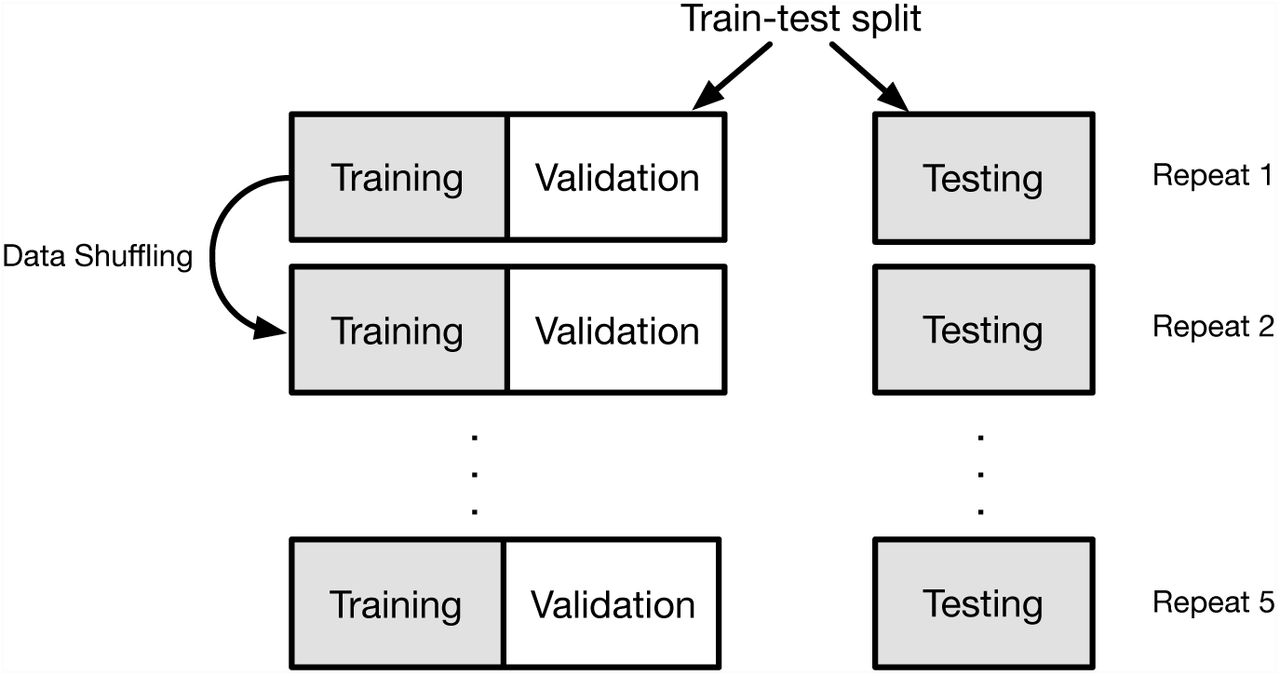
There are multiple factors that may influence the performance of a classifier. These include the choices regarding the algorithm, the values of associated hyperparameters and the feature set to be used for classifying. In addition, there is there are design considerations concerning selection of data for training and subsequent testing. The processes we employed for both the one- and two-class classification problems are illustrated in Fig 7. Our core algorithm choices are described above. Our experimental design for involved training our classifiers on data derived from mouse chromosome 1 only. For each algorithm, we used cross validation to tune the hyperparameters and optimize the classifier. For every cross validation iteration, we firstly perform a random train-test split, and divide our data sets into training data and testing data. Then inside the training data, we further split training data to actual training data and validation data (Fig 8). We train the classifier on actual training data, set hyperparameters on validation data and finally evaluate classification performance on testing data. Within each validation process, we compared algorithm performance with different hyperparameter values and the hyperparameter generating the best performance for the available data was saved. For each classification experiment, this process was repeated 5 times.

Overview of classifier algorithm evaluation. (a) Two-class classification includes labelled spontaneous and ENU-induced germline point mutations in the training data. (b) One-class classification includes only spontaneous germline point mutations in the training data. For both approaches, training data was limited to mutations occurring on mouse chromosome 1.
Procedure of cross validation. For each cross validation iteration, the data were shuffled and then divided into three segments, one for training, one for validation and the third one for testing. For each experiment, performance of algorithms with different hyperparameter were compared. The best algorithm for the available data was saved. The process was repeated 5 times.
For the LR classification, the hyperparameter C is the trade-off regularization parameter which trades off misclassification of training examples against simplicity of the decision surface. A low C makes the decision surface smooth, while a high C aims at classifying all training examples correctly by giving the model freedom to select more samples as support vectors. We considered candidate C options from the log-scale of: 0.01, 0.1, 1, 10, 100. The C value that resulted in the best performance (please refer to Classifier performance evaluation section), was chosen for all subsequent analyses.
For the Naïve Bayes classification, the hyperparameter alpha is the Laplace parameter used to smooth categorical data. We considered candidate alpha options of: 0.01, 0.1, 1, 2, 3. The value of alpha which resulted in the best performance was chosen for all subsequent analyses.
Classifier performance evaluation
We evaluated classifier performance using the area under the receiver operating characteristic curve (AUC). One of the advantages of using AUC score as the performance measure is that the score does not require choice of a cutoff threshold. Many binary classification algorithms compute a series of performance scores (e.g. overall accuracy, sensitivity, and specificity), and they classify based upon whether or not the score is above a certain threshold. Therefore, as the choice of threshold is of particular importance in these scoring schemes, shifting of the threshold may dramatically alter the score and thus the performance of a classifier. AUC score has the advantage of illustrating the trade-off between sensitivity and specificity for all possible thresholds rather than just the one that was chosen by the modeling technique. Here, the AUC scores of the different experiments are reported and we interpret a larger AUC score as indicating better classification performance.
The effect of increasing the number of examples during training
The whole classification process is achieved by implementing training and testing phases. In the training phase, a set of data and their respective labels are used to build a classification model. In the test phase, the trained classifier is used to predict new cases. Overlap sampling between training and testing data will make the prediction performance of a classifier overly optimistic, because of the overfitting problem. To avoid the overfitting situation, for each experiment, to start with, both ENU-induced mutations and mouse germline mutations are split into two non-overlapping sets for training and testing.
The accuracy of a classifier improves with the number of observations used to train the algorithm. This improvement tends to be rapid initially, and then when the training size is sufficient to a point, the improvement decreases gradually. The “learning curve” is used to describe this phenomenon, and is used to estimate the number of samples needed to train a particular classifier to achieve its optimal accuracy (Mukherjee et al., 2003). To plot learning curves and find the desired training size, after selecting a specific classifier and set of features, we used progressively larger samples of observations to train the classifier and then plot accuracy performance against the number of training observations.
Availability of data and materials
The pre-processed data used in this study are available at Zenodo https://zenodo.org/record/1204695 under the Creative Commons Attribution-Share Alike license. Data files are typically gzip compressed standard formats, e.g. tab delimited text files, fasta formatted sequence files. The scripts performing the data sampling and applying the analyses reported in this work are freely available at Zenodo https://zenodo.org/record/1283516 under the BSD clause-3 license.
Acknowledgements
We thank B Kaehler, H Simon and H Ying for comments on earlier versions of the manuscript.
References


