

Abstract
Sequence-to-sequence alignment is a widely-used analysis method in bioinformatics. One common use of sequence alignment is to infer information about an unknown query sequence from the annotations of similar sequences in a database, such as predicting the function of a novel protein sequence by aligning to a database of protein families or predicting the presence/absence of species in a metagenomics sample by aligning reads to a database of reference genomes. In this work we describe a deep learning approach to solve such problems in a single step by training a deep neural network (DNN) to predict the database-derived labels directly from the query sequence. We demonstrate the value of this DNN approach on a hard problem of practical importance: determining the species of origin of next-generation sequencing reads from 16S ribosomal DNA. In particular, we show that when trained on 16S sequences from more than 13,000 distinct species, our DNN can predict the species of origin of individual reads more accurately than existing machine learning baselines and alignment-based methods like BWA or BLAST, achieving absolute performance within 2.0% of perfect memorization of the training inputs. Moreover, the DNN remains accurate and outperforms read alignment approaches when the query sequences are especially noisy or ambiguous. Finally, these DNN models can be used to assess metagenomic community composition on a variety of experimental 16S read datasets. Our results are a first step towards our long-term goal of developing a general-purpose deep learning model that can learn to predict any type of label from short biological sequences.
Main Text
Many important problems in bioinformatics can be framed as determining a mapping from short biological query sequences to salient categorical or numerical labels. Taxonomic classification or binning; prediction of protein function, gene properties, or pathogenicity; read filtering for contaminants; RNA-seq quantification; and antibiotic resistance profiling all fall in this category. While it may be possible to solve each such problem in isolation, we instead aim to develop a single machine learning model capable of solving a wide range of these problems. This end-to-end approach has potential to learn directly from sequencing data, increase runtime efficiency, reduce the need for human effort and problem-specific information, and discover novel features.
The flexibility of artificial neural networks make them a promising choice for building such a general tool. Our end-to-end deep neural network (DNN) approach reframes the sequence-labeling problem as condensing relevant information from numerous labeled sequences into the weights of the network. The DNN architecture we apply leverages depthwise separable convolutions (Figure 1), which have been shown empirically to use parameters more efficiently than regular convolutions in architectures for both vision (for example, Xception12 and MobileNets14) and language processing (e.g. SliceNet13). We explore the plausibility of replacing popular database-matching tools with this deep learning solution by studying its application to a well-characterized problem of practical importance: predicting species-level taxonomy directly from short reads of 16S ribosomal DNA.

The neural network architecture used in this study consists of three depthwise separable convolutional filters followed by two or three fully-connected layers (in green), which are tiled as needed along the length of the input and combined via an average pooling layer prior to the softmax output layer.
Ribosomal RNA sequencing has been an essential tool for studying microbial phylogeny since its introduction more than forty years ago.1,2 Massive cost reductions due to recent improvements in sequencing technology have made it possible to develop large, public repositories of high-quality 16S sequencing data; the Human Microbiome Project alone contains more than 14 terabytes of data and thousands of taxonomically characterized communities.3,4 This growing data richness enables new types of research probing composition, diversity, and function of complex microbial communities, but also necessitates creating analysis methods capable of efficiently handling these large sequencing datasets. Existing tools for read-based taxonomic classification such as the Ribosomal Database Project (RDP) SeqMatch tool,8,33 mothur,6 and QIIME7 typically rely on explicit sequence matching against identified genomic sequences via a k-mer, Basic Local Alignment Search Tool (BLAST),29,30 suffix tree, and/or edit distance approach.
There are few machine learning models for read-level classification, many of which still tend to incorporate explicit sequence similarity. For example, the popular RDP Classifier8 uses a naive Bayes approach to provide taxonomic assignments for 16S sequences from superkingdom to genus based on relative frequencies of 8-mers. Similarly, La Rosa et al.9’s probabilistic topic modeling approach classifies 16S rRNA sequences from phylum to family by exploiting the frequencies of fixed-length k-mers. These and other such k-mer-based approaches are limited by the loss of positional information and the complexities of dealing with noise and bias. Indeed, neither of the aforementioned works discuss handling noisy input sequences.
Neural networks have not yet been thoroughly explored as an alternative to explicit sequence matching. One of the earliest studies in this direction uses three-layer fully-connected neural networks with backpropagation to predict species membership from DNA barcode sequences.10 Although this approach yields more accurate species assignments than alignment or distance search on two simulated datasets and attains high accuracy on two empirical datasets, its practicality is limited due to the work’s small scale (fewer than ten distinct species at a time) and its focus on long (400-750 base pair) reads. Recent work by Khawaldeh et al.11 shows that a convolutional neural network can achieve over 99% accuracy at the order level of the taxonomic hierarchy, though their prediction task was limited to nine distinct labels and they offered no direct comparison to existing approaches nor validation on experimental reads. Ultimately, this past work provides initial evidence in support of neural networks, but falls short of providing meaningful guidance on whether a modern deep learning solution for read labeling has any practical advantages over popular sequence matching approaches.
To our knowledge, no previous work demonstrates that neural networks can classify genomic sequencing data of realistic scales at fine taxonomic resolution, or provides an in-depth comparison to existing machine learning and sequence matching techniques. We show that our proposed neural network architecture for sequence labeling scales successfully to more than 13 thousand distinct species without requiring explicit sequence similarity features, and moreover that it can accurately analyze both synthetic and experimental read data. Specifically, we find that these learned, discriminative classifiers achieve performance comparable to that of traditional alignment tools for long, relatively noiseless queries, but produce more accurate read-level taxonomic labels when query sequences are particularly ambiguous or noisy, even when we restrict our attention to a range of noise rates (0.5% to 10%) produced by next-generation sequencing technologies in practice. We use these results to understand the conditions under which this deep learning solution is most advantageous, and conclude by discussing the generality of our approach and associated analysis methods.
Results
Training Performance
We first explored, for each of five read lengths L = {25, 50, 100, 150, 200}, whether a neural network, DNNL, of the structure in Figure 1 is capable of learning to predict accurate read-level labels. We trained each model DNNL, independently on a set of synthetic reads, NCBIL, generated by extracting all subsequences of length L from a set of 19,851 16S references sequences from NCBI.20 Figure 2(a) shows that, overall, classification accuracy increased as a function of read length: as read length increased from 25 to 200 base pairs, the Bayes optimal classification rate rose from 19.8% to 72.4% for the species task and 49.2% to 96.3% for the genus task. Each neural network achieved species classification accuracy within 2.0% of the maximum achievable accuracy on the training set, which shows that these models are capable of learning the underlying read-level mapping reasonably well. For comparison, species-level classification accuracies using the Burrows-Wheeler aligner (BWA)25,26 fell, on average, 4.6% below Bayes optimal. Higher-order predictions obtained by marginalizing the models’ probability distributions were also highly accurate, coming within 1.0%, 0.6%, and 0.5% of Bayes optimal accuracies at the genus, family, and order levels, respectively. On the remaining class, phylum, and superkingdom classification tasks, DNN25 attained 84.4%, 90.0%, and 99.9% read-level accuracies, whereas the remaining models surpassed 95.7% accuracy on all these tasks.


(a) The results of each neural network DNN200, DNN150, DNN100, DNN50, and DNN25 on its training set (NCBI200, NCBI150, NCBI100, NCBI50, and NCBI25, respectively) on the order, family, genus, and species predictions tasks compared to the Bayes optimal accuracy rate (‘opt’), (b) The same as (a) when all methods are evaluated on reads from NCBI250.
Evaluating each neural network on NCBI250 revealed the impact of read length during training (Figure 2(b)). Overall, the models performed well on these 250 base pair reads, particularly at less granular taxonomic ranks: DNN25 attained 98.3% read-level accuracy on order prediction, and the remaining networks (DNN50, DNN100, DNN150, and DNN200) achieved over 99.7% read-level accuracy on order, class, phylum, and superkingdom classification. Performance was more variable at finer resolutions: read-level species accuracies ranged from 64.1% to 74.5%, with those for DNN25 and DNN50 being noticeably lower (6.1% and 13.6% below Bayes optimal, respectively). On the other hand, DNN200, DNN150, and DNN100 all came within 4.1% of this species-level Bayes optimal classification rate. We found that DNN200 classified the 250 base pair reads most accurately at every taxonomic rank, achieving 77.7%, 97.8%, and 99.5% accuracy for the species, genus, and family prediction tasks.
Solely examining classification rates obscures the probabilistic nature of the deep learning models’ predictions. To investigate whether these probability assignments themselves have any interesting properties, we compared the probability weights assigned by DNN100 across the length of a fixed reference sequence. Figure 3(a) shows that DNN100 made no within-genus mistakes on synthetic reads from the Salmonella enterica reference sequence, whereas in Figure 3(b) within-genus mistakes were common in regions of the reference sequence where DNN100 assigned low probability weights to the true Salmonella bongori label. However, in both of these cases we found that the neural network predicted the correct species with high confidence for synthetic reads within 100 base pairs of the hypervariable regions (identified using analysis by Chakravorty et al.27 and the E. coli coordinate from Brosius et al.28).


Probability weight assigned to the correct species label by DNN100 for every 100 base pair subsequence of (a) Salmonella enterlca (RefSeq ID NR_116126.1), (b) Salmonella bongori (NR_116124.1), and (c) Streptomyces libani (NR_042301.1) reference sequences. Offset from the beginning of the reference to the start of the subsequence is specified on the x-axis, and color represents whether DNN100’s most confident prediction is the correct label (yellow), another species label in the correct genus (cyan), or a species outside the genus (blue), (d) The genus-level probability weights assigned by DNN100 to the Streptomyces label for the same reference sequence as (c).
We repeated this analysis on a Streptomyces libani reference sequence and found that the model’s output probabilities followed an entirely different trend (Figure 3(c) and (d)). Unlike in the Salmonella cases, the probability the model assigns to the correct species label remains below 0.36 across the reference. Moreover, aside from a few correct assignments near the labeled hypervariable regions, within-genus mistakes dominate Figure 3(c). Indeed, we found the model’s genus-level predictions to be both accurate and confident on the same synthetic reads from the reference sequence; Figure 3(d) shows that DNN100 made no genus mistakes and assigned at least 0.8 probability to the Streptomyces label everywhere except for a small region between V2 and V3.
Noise Experiments
Experimental reads inevitably contain noise. To better understand how our models would behave on noisy reads, we retrained DNN25, DNN50, DNN100, and DNN200 on synthetic reads from a sample of 12,598 of the species in the NCBI training data with base-flipping noise randomly injected into the input examples. Including noise at a rate of 4% during training reduced DNN100’s read-level species accuracy on noiseless training examples from 52.7% to 52.0%. Moreover, when we trained DNN100 with 16% noise, it classified species correctly for only 46.9% of these noiseless training examples, which is lower than the 49.1% achieved by using BLAST. DNN25, DNN50, and DNN200 tended to follow the same trend: increased noise during training decreased model accuracy on noiseless reads and, for sufficiently high noise rates, reduced it below the accuracy obtained by alignment. However, performance differentials tended to decrease in magnitude as read length increased, particularly at the genus level where performance gaps between the Bayes optimal classifier and the better of the alignment baselines decreased monotonically from 9.6% to 1.4%. This same trend is present in Figure 4: the pairwise differences between model and alignment performance on the task of placing the reads from held-out species into accurate genera decreased as read length L increased.
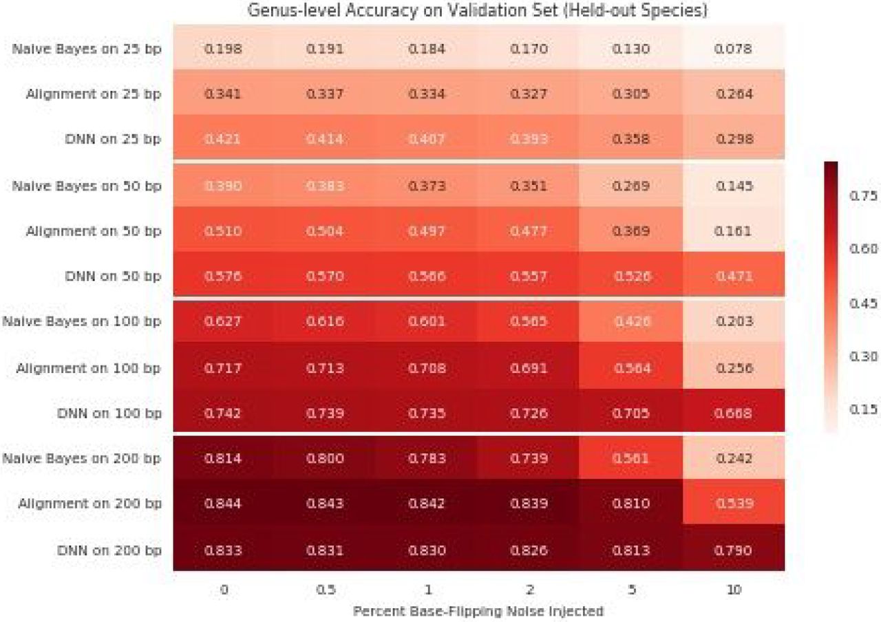
Heatmap showing the read-level accuracy of our deep learning approach relative to naive Bayes and alignment approaches on the task of assigning noisy reads from held-out species to the correct genera. Here, alignment represent the better of our BLAST and BWA baselines, and each cell is labeled with the proportion of reads placed into the correct genus when the corresponding method (y-axis) is used to assess reads corrupted by the given noise rate (x-axis).
Figure 4 reveals the differential impact of corrupting the reads from the held-out species with noise on naive Bayes and alignment approaches relative to our deep learning approach across 24 different read length and noise rate pairs. In all cases, we found our neural networks preferable to a naive Bayes baseline modeled on the RDP Classifier,8 with individual gains ranging from 1.9% to 54.8%. Our deep learning models additionally outperformed alignment baselines in 20 of these 24 experiments. Our improvement over the best alignment approach ranged from 0.3% to 41.2%, with performance gains of 5.3%, 15.7%, 14.1%, and 0.3% on 25, 50, 100, and 200 base pair queries with 5% noise, respectively. In contrast, for the 4 low-noise experiments on 200 base pair reads, we found our model performed comparably to BLAST, which attained no more than a 1.3% advantage in these scenarios. Interestingly, our neural networks reached relatively high read-level genus classification accuracies on the reads from held-out species even in settings where BWA failed to align a significant portion of the reads. For example, BWA achieved less than 3% read-level genus accuracy on 200 base pair reads from held out species with 5% or 10% injected base-flipping noise, whereas our deep learning approach obtained 79.0% and 81.3% accuracies on these same tasks.
Mock Community Evaluation
Although our experiments with base-flipping noise provided valuable insights about how our deep learning approach might perform in the presence of real sequencing errors, all experiments thus far have used simulated reads pulled directly from 16S reference sequences. To validate our method on real experimental reads, we used one of our best-performing models trained with reverse complements to analyze empirical amplicon sequencing data from microbial mock communities.
In Figure 5, we plot our community reconstructions based on the outputs of DNN 100 for 57 sets of mock community sequencing data from Nelson et al.,22 Schirmer et al.,31 and D’Amore et al.23 For six 20-organism mock community replicates, we found that our model-based estimation was able to perfectly reconstruct the list of 17 genera for 5 of the 6 replicates. At the species level, our method identified, on average, 21.8 distinct species (16.3 truly present and 5.5 false discoveries). For the remaining 51 mock community sequencing datasets, we correctly identified on average 36.0 of 45 genera and 32.6 of 56 species based on the model’s probability assignments. At the genus level, we consistently failed to recover Nanoarchaeum (a label which is not contained in our NCBI dataset) in addition to 5 other Archaeal genera: Methanocaldococcus, Pyrococcus, Sulfolobus, Archaeoglobus, and Ignicoccus. In addition, Nostoc and Leptothrix are consistently mistaken for within-family false positives: Cylindrosperum and Roseateles, respectively.

(a) The number of total predictions, true positives, and false positives contained in the species-level reconstructions calculated using model-based estimation with DNN100 for 6 replicates of the 20-organism mock community from ENA study PRJB4688 and 51 runs of the 59-organism community from PRJEB6244. (b) The same as (a) for the genus-level reconstructions.
Overall, across all 57 sets of amplicon sequencing data, our model-based estimation method attained mean positive predictive value and sensitivity of 0.657 and 0.610 at the species level, and 0.908 and 0.824 at the genus level. Comparing to analyses by D’Amore et al.,23 our approach discovered fewer spurious genera than the RDP Classifier (4.1 compared to 55.6) without a large decrease in the number of accurately recovered genera (36.0 versus 39.3), though the RDP Classifier was trained on a much more comprehensive dataset of nearly 169 times as many reference sequences. In addition, our model’s consistent inability to recover certain Archaeal genera is likely due to the “failure of the V1-V9 primers in amplifying the Archaea.”23
Discussion
Our results indicate that the deep neural network model we proposed is capable of solving read-labeling problems. Specifically, the models we trained obtained near-optimal species classification performance and marginalized accurately to higher-order taxonomic ranks (Figure 2). Pooling provides important flexibility for our models and makes it possible to apply them on read lengths they were not trained on. However, as can be seen in Figure 4, using a minimum read length that is too small can have some disadvantages in practice. In particular, when evaluated on noiseless 250 base pair reads from our NCBI references, the model trained on 25 base pair examples is noticeably less accurate below the order level than models trained on longer reads. The models trained on longer reads achieved upwards of 99.7% read-level accuracy on order classification, a result comparable to the 99.6% accuracy reported in Khawaldeh et al.11 even though our models were optimized for species prediction and we considered a much larger number of possible order labels (202 distinct order labels compared to 9).
Agreement between the models’ individual predictions and what we know about the 16S gene provides further evidence of learning. We would expect classification to be more difficult on the gene’s conserved regions, and indeed Figure 3 shows that queries which yield predictions that are more confident in the correct label tend to cover parts of the hypervariable regions. Moreover, for Streptomyces libani, one of 681 species from this most prevalent genus, our model places low probability mass on the correct species, despite making accurate, highly-confident genus assignments along the same reference sequence. This suggests that the model’s probability mass is divided amongst multiple closely-related Streptomyces species which cannot be disambiguated due to an insufficient proportion of distinctive reference sequence. In other words, the model is both less confident and less accurate on highly-conserved regions. However, differential coverage in the training data can also have an impact: the model made many within-genus mistakes for the less prevalent Salmonella bongori (2 references) but none for Salmonella enterica (11 references). As such, a more robust training or inference scheme which properly adjusts for skewed coverage might improve the quality of these predictions.
Through experimentation with base-flipping noise, we delineate a particular problem space within bioinformatics--where inputs are short and noisy--within which our learned, discriminative neural networks are preferable to sequence-matching. For every combination of read lengths and noise rates we tried in Figure 4, our deep learning approach was more accurate than the naive Bayes baseline, a reimplementation of the RDP Classifier’s underlying method. Though alignment baselines were more competitive, consistent advantages on 25 and 50 base pair queries, as well as large performance differentials in higher noise-rate scenarios (see the bottom right corner of Figure 4), still established our deep learning approach as preferable particular data regions. The fact that our method demonstrates the most significant advantages over alignment for shorter, noisier data is consistent with findings that the RDP Classifier and RDP SeqMath tools have nearly identical overall error rates on long and near-full-length test sequence from the 16S gene.8 Some relatively straightforward alterations to the deep learning approach we have outlined (for example by leveraging the hierarchical nature of taxonomic labels via multi-task learning or hierarchical softmax or by allowing users to explicitly include alignment mapping features as additional model input) might allow it to outperform in this setting, as well.
These advantages on short and noisy reads offer some guidance into how useful our proposed approach might be in practice. For example, we can think of base-flipping noise as simulating several intrinsic sources of difference, such as diversity, low quality reference sequences, sequencing errors, and subspecies variability. Moreover, Figure 2 shows a substantial decrease in the Bayes optimal classifier’s genus misclassification rate (from 50.8% to 3.7%) as a function of read length, which suggests that read length acts as a proxy for the number of queries with ambiguous label assignments. As such, our results in the presence of base-flipping noise suggest that our deep learning approach might be able to improve analytical results on experimental data with high levels of inherent error or ambiguity.
Our mock community analyses give us reason to believe that these potential practical advantages could be realized, as they establish that the success of our proposed deep learning approach to read-level taxonomic labeling extends from synthetic read sets to real next-generation sequencing data. Specifically, we showed that outputs from DNN100 on mock community sequencing reads could be integrated successfully into downstream analytics related to species-and genus-level mixture estimates (Figure 5). Indeed, the resulting community reconstructions were relatively robust to different primers, library preparation methods, DNA polymerases, and amplification targets employed by studies PRJEB4688 and PRJEB6244.
We have thus defined a new deep learning approach for solving sequence-to-label prediction problems in bioinformatics which uses a depthwise separable convolutional neural network to assign database-derived labels to query sequences in a single step. This approach to matching short biological sequences to meaningful labels provides an alternative to the widely-used two-phase approach of first aligning an unknown query sequence to a database of known reference sequences and then inferring label assignments from the annotations of similar database sequences. By focusing on a well-characterized problem of practical importance--species-level classification of reads from 16S ribosomal RNA--we established that 1) our depthwise separable convolutional network is capable of learning to accurately solve the read-level species identification problem, 2) this deep learning approach consistently outperforms alignment in two specific data regimes, and 3) this success extends to empirical metagenomic data generated using a wide range of experimental procedures. Figure 6 clarifies another way to intuit these results: the introduction of this new deep learning approach effectively extends the data regions within which we can perform accurate analyses, in particular by contributing large accuracy improvements over sequence alignment in particular data settings.

Contour plots distinguishing data regions (indexed by read length and noise rate) of high accuracy (darkest) from those of lower accuracy (lightest) for alignment methods (left) and our deep learning approach (right) based on an interpolation on the results presented in Figure 4. The rightmost plot gives contours for the advantage of our deep learning method over alignment over the same data regions, where here darker contour represent a larger advantage.
Beyond accuracy, this deep learning solution has the potential to make significant contributions in terms of the resources and performance required for labeling analyses. The model we used for our inference on mock community sequencing data requires about 1.1 G of storage for its parameters and consists of approximately 1.2 million floating-point operations per query. While actual performance levels may vary with query length and application, leveraging hardware accelerators for machine learning could allow this deep learning approach to process roughly 13 million queries per second on a V100 GPU or 156 million queries per second on a Cloud TPU. Perhaps even more enticing compared to alignment approaches is its suitability for being adapted to mobile. In general, modern smartphones are capable of processing more than 10 billion floating-point operations per second, which translates to upwards of 9 thousand queries per second. However, given the close similarity of our proposed architecture to those currently used for image processing, it should be possible to improve this estimated performance by directly leveraging work, for example by Howard et al.14, to streamline vision models for mobile and embedded applications.
Finally, we emphasize that the model and associated analysis method we outline in the current study are highly general, making this new approach an excellent candidate for replacing existing sequence-to-sequence alignment approaches on many large-scale bioinformatics problems, particularly those where data is inherently ambiguous or noisy such as the analysis of bisulfite sequencing, viral and/or microbial DNA for strain identification, immune-mapping, cell-free DNA, and ancient DNA. Indeed, this work was the basis of our team’s submission to the recent PrecisionFDA Pathogen Detection Challenge (https://precision.fda.gov/challenges/2I which confirmed through a blinded, independent evaluation that our deep learning approach performs reasonably well on data from genes beyond 16S and for several other labeling tasks (Appendix 5). Competitive accuracies for strain and serotype prediction strongly suggest that this technology is generalizable, though there is room for additional improvements over this initial method (shown by a performance gap for multilocus sequence typing). We plan to incorporate such improvements into a submission to the current MOSAIC challenge (July 25, https://platform.mosaicbiome.com/challenges/6 Overall, the current study provides an important initial proof-of-concept for and acts as a first step towards our long-term goal of developing a general-purpose deep learning model that can learn to successfully perform any task framed as the assignment of labels to short biological sequences.
Methods
NCBI Data
We used public reference sequences from the NCBI RefSeq Targeted Loci Project20 to generate synthetic reads. Specifically, we used 19,851 16S ribosomal RNA sequences provided in NCBI BioProjects 33175 and 33317 (downloaded 2017-11-27), of which 18,902 are bacterial and 949 are archaeal. These references have an average length of 1,454.13 base pairs, although individual sequences vary from 302 to 3,600 base pairs.
Let NCBIL denote a set of synthetic reads of length L generated from our NCBI reference sequences. For L = {25, 50, 100, 150, 200}, we construct this set by extracting subsequences of L base pairs from each reference sequence in a sliding window fashion, and pairing each such “read” with taxonomic labels at the superkingdom, phylum, class, order, family, genus, and species levels extracted from NCBI Taxonomy Browser.21 During this extraction and labelling process, we excluded 129 reference sequences whose reported taxonomic labels violated the tree structure of the taxonomy, and as such each set NCBIL represents 13,838 distinct species, 2,768 distinct genera, 479 families, 202 orders, 91 classes, and 38 distinct phyla (see Appendix 1 for more details).
Each read in NCBIL is a short sequence of canonical nitrogenous bases (A, C, T, G) and IUPAC ambiguity codes (K, M, R, Y, S, W, B, V, H, D, X, N). We one-hot encoded each canonical base as a four-dimensional vector and resolved each ambiguity code to the appropriate probability distribution over these four bases (Extended Data Figure 1). Note that this approach to input encoding does not make use of any quality scores; it would be straightforward to extend our approach to include this information, for example by using an extra input channel. Similarly, we one-hot encoded the species identity as a 13,838-dimensional vector.
For model selection, we split NCBIL into three smaller subsets: NCBI-0L, NCBI-1L, and NCBI-2L. We constructed NCBI-0L by first taking a random sample of 90% of the species in each genus (selecting at least one species per genus), then sampling 90% of the reads for each selected species. The remaining 10% of the reads for these species form NCBI-1L, and NCBI-2L contains all the reads for the 10% of species not selected for NCBI-0L. Appendix 2 gives an example of the read and label contents of these subsets for L=100.
Mock Community Data
In addition to our synthetic NCBI read sets, we used experimental 16S mock community sequencing data to evaluate our trained classifiers. We obtained experimental reads from Nelson et al.,22 Schirmer et al.,31 and D’Amore et al.23 through studies PRJEB4688 and PRJEB6244 in the European Nucleotide Archive.24
The mock community in study PRJEB4688 was developed by the Human Microbiome Project3 to contain equal concentrations of 20 bacterial species. In our analyses, we used the three Illumina MiSeq single-ended replicates, ERR348713-5, and the three corresponding paired-end replicates, ERR619081-3. Read lengths in these replicates vary from 225 to 384 base pairs. In contrast, all reads in the 51 mock community sequencing runs from study PRJEB6244 are 250 base pairs long, and the communities sequenced contain known amounts of DNA from ten members of Archaea and 49 bacterial strains. See Appendix 3 for more details regarding the composition of these communities or properties of the replicates.
Depthwise Separable Convolutions
In preliminary experiments, we found that artificial neural networks employing depthwise separable convolutions were effective at predicting taxonomic labels directly from short reads of 16S rRNA gene, even at the species level. Initially studied by Sifre & Mallat,15 depthwise separable convolutions can be thought of as convolutional feature extractors that separate the task of learning spatial features from that of integrating information across channels. This is accomplished by decomposing a regular convolution into two sequential operations: a spatial convolution applied independently over each channel of the input followed by a pointwise convolution across channels. For DNA sequences, we use of 1D depthwise separable convolutions, which can be formalized as follows given input x with C channels and a filter of width F:
 where W denotes a weight matrix and ∘ represents element-wise multiplication.
Model Architecture
For this read-level prediction problem we used an architecture comprised of 3 layers of depthwise separable convolutions followed by two to three fully-connected layers, a pooling layer, and a softmax output layer that produces a probability distribution over the 13,838 possible species labels. Each convolutional and fully-connected layer is followed by an activation function and dropout regularization.32 Specifically, we use leaky rectified-linear activation:
 where the slope a ∈ (0,1) for each model is as in Extended Data Table 1.
To compute a new probability distribution over higher taxonomic labels, we simply marginalized the species-level distribution produced by the softmax layer by summing the probability assigned to all species under each taxon. Moreover, to evaluate longer reads we tiled the fully-connected layers as necessary and depended on the pooling layer to combine the intermediate outputs before the softmax. We found that average pooling worked the best for this application (see Appendix 4 for more details), and as such all models presented in the current study used an average pooling layer.
Although the pooling layer allows our model to tolerate some variation in read length, we nevertheless found it useful to train multiple models optimized for different read lengths. Extended Data Table 1 shows the best configuration we found for each read length. See Appendix 2 for more details on model selection and tuning.
Training and Implementation
We implemented our neural networks using the open-source software library TensorFlow.16 To train the models, we randomly initialized the parameters for each layer according to a truncated random normal distribution with standard deviation given by  where S is the weight initialization scale (see Extended Data Table 1) and N is the number of inputs to the layer. On each iteration, we used a randomly selected mini-batch of 500 read and species label pairs to update the model parameters, with the objective to minimize cross entropy between the true species identities and the model’s predictions. These parameter updates are computed and applied using TensorFlow’s implementation of the ADAM optimizer,19 with gradients clipped to have norm at most 20.
In many of our experiments we injected random base-flipping noise into input read sequences before supplying them to the model. We have two motives for doing so. First, the noise can act as a regularizer to avoid overfitting to our synthetic reads. Second, it enables exploration into whether our models perform better on errorful reads at test time when noise is included at train time. We injected this noise by mutating each base b in a given read with fixed probability r according to the following rule:
If b is a canonical base:
Flip b to one of the other three canonical bases with equal probability.
Otherwise:
Flip b to one of the four canonical bases with equal probability.
The sequence produced by performing these random flips is then taken as input instead of the original sequence. We trained models with five different rates of base-flipping noise r = {0%, 2%, 4%, 8%, 16%} and evaluate on data with injected noise rates of r = {0%, 0.5%, 1%, 2%, 5%, 10%}. We found that models failed to train when base-flipping noise was increased to a rate of 32%.
Bayes Optimal Classifier Baseline
We used the Bayes optimal classifier to compute upper bounds for read-level accuracy. Here, Bayes optimal accuracy is the maximum accuracy achievable by perfect rote memorization of all (read, species label) pairings seen during training. Let T be a fixed set of training examples. We compute the Bayes optimal classification rate as follows:
Partition T into subgroups T1,T2, …, TN of (read, species label) pairs so that N is the number of distinct read sequences in T and all the training examples in T which share the same read sequence are contained in the same subgroup Ti
Define counti(s) as the number of times the species label s appears in the subgroup Ti and compute

Let |T| be the total number of reads in T and take
as the final accuracy


We repeat this process for higher taxonomic ranks to provide Bayes optimal accuracy bound on the superkingdom, phylum, class, order, family, and genus prediction tasks.
Alignment Baselines
We used BLAST and BWA to compute practical performance baselines based on alignment against the original reference sequences. These baselines reflect the accuracy of randomly guessing a label for each read from the set of labels associated with all alignment mappings that are equally good. Again taking T to be a fixed set of short reads, we computed the BWA baseline as follows:
Let a be an alignment mapping, so that aref is the reference sequence involved in the given alignment and aed is the edit distance score for the mapping
Set accuracy = 0 and for each read x ∊ T
Use BWA to assign a set of mappings A and primary mapping a* to the read x
If A is empty, accuracy ± 0; otherwise:
Take
accuracy ±
where C is the number of times the true label for read x appears in the set of groundtruth labels for {aref|a ∊ A*}
Let |T| be the total number of reads in T and take
as the final accuracy rate BLAST baseline accuracy in computed in the same way by simply replacing the comparison in 2b with one which checks for bit scores which are at least as large as the bit score of the best mapping.


Naive Bayes Baseline
We implemented a naive Bayes classifier based on exact 8-mer matches of query reads to the original references sequences, akin to the RDP Classifier.8 Briefly, we transformed input sequences into vectors indicating the presence or absence of each possible 8-mer subsequence. For each such 8-mer, the prior probability used for its presence was the fraction of all training set reads that contain one or more instances of the 8-mer with pseudocounts of 0.5 and 1 in the numerator and denominator, respectively, as described previously.8 The genus-specific conditional probability of each 8-mer was calculated with respect to the subset of training set reads drawn from the genus with a numerator pseudocount of the word-specific prior probability.8
The 8-mer vector representation for each read handled IUPAC ambiguity codes by assigning each possible DNA 8-mer a fractional presence. For example, the 9 base pair sequence ‘ AAAAAAAAN’ was transformed into a vector with four non-zero entries: AAAAAAAC, AAAAAAAG, AAAAAAAT all with weights 0.25, and AAAAAAAA with weight 1.0 (because this 8-mer occurs exactly in the sequence). We found that incorporating these ambiguous bases incurred a slight loss in accuracy compared to ignoring 8-mers with non-DNA characters for long reads with little noise, but improved accuracy for short or noisy reads (data not shown).
Mock Community Evaluation
We used the following iterative mixture estimation method to attempt to predict community composition from a set of raw sequencing reads:
Let DNN be a fixed neural network model and initialize a matrix of read-level probabilities P where the row Pi = DNN(xi) where xi is the ith read in the set of raw sequencing reads
Initialize a vector of mixture estimates E as the uniform distribution over all possible species labels
For each iteration:
Compute matrix T where
Update


where again we use ∘ for element-wise multiplication. We used this approach with DNN100 trained with 4% base-flipping noise to reconstruct mock communities based on sequencing data by taking the final E as our set of mixture estimates and taking the list of species with estimated mixture fractions of at least 0.001 as the predicted set of community members. Moreover, we repeated this process to estimate the genus-level composition by marginalizing to the genus level and initializing E as a uniform distribution of the appropriate size. For the purposes of this analysis, we ignored pairing information and treated each read as independent. We performed this procedure using 10,000 reads and 75 iterations for the smaller mock community, and 20,000 reads and 150 iterations for the larger one; in cases where the specified number of reads is larger than the current read set, we simply use the entire replicate.
Code Availability
TensorFlow code for building and training new models with the proposed architecture is available through the TensorFlow Research Models GitHub repository (https://github.com/tensorflow/models/tree/master/research). The released code can be used to train new models and produce model checkpoint files. If desired, one can create a custom evaluation loops which leverage these checkpoints. Those interested in other capabilities should contact seq2species-interest{at}google.com.
Data Availability
The datasets supporting the findings of this study were derived from the following public domain resources: NCBI RefSeq Targeted Loci Project
(https://www.ncbi.nlm.nih.gov/refseq/targetedloci); ENA Study: PRJEB6244
(https://www.ebi.ac.uk/ena/data/view/PRJEB6244); ENA Study: PRJEB4688
(https://www.ebi.ac.uk/ena/data/view/PRTEB4688) Data converted to TensorFlow TFRecord format is available in a bucket on Google Cloud Storage
Supplementary Information
Supplementary information is available in a separate supplementary materials document.
Author Contributions
A.B., G.D., C.F. and M.D. conceived of and designed the study. A.B., C.F., D.H.A., R.P., C.Y.M. and P.C. performed experiments. A.B., G.D., D.H.A., E.D., R.P., C.Y.M., P.C. and M.D. analyzed and interpreted results. A.B., G.D., E.D., R.P., C.Y.M. and M.D. wrote the manuscript.
Author Information
Correspondence and requests for materials should be addressed to mdepristo{at}google.com or seq2species-interest{at}google.com.
The authors declare the following competing interests: the authors are employees of Google.
Acknowledgements
For their early input, which helped to frame the initial problem and understand potential applications, we thank Adam Roberts, Cinjon Resnick, and C. Rob Young. For their sharing of experimentalist perspectives on the problem, we thank Mauricio Carneiro, Vanessa Ridaura, and Roie Levy. This work was supported by internal funding.


