

Abstract
The average power of rhythmic neural responses as captured by MEG/EEG/LFP recordings is a prevalent index of human brain function. Increasing evidence questions the utility of trial-/group averaged power estimates, as seemingly sustained activity patterns may be brought about by time-varying transient signals in each single trial. Hence, it is crucial to accurately describe the duration and power of rhythmic and arrhythmic neural responses on the single trial-level. However, it is less clear how well this can be achieved in empirical MEG/EEG/LFP recordings. Here, we extend an existing rhythm detection algorithm (extended Better OSCillation detection: “eBOSC”; cf. Whitten et al., 2011) to systematically investigate boundary conditions for estimating neural rhythms at the single-trial level. Using simulations as well as resting and task-based EEG recordings from a micro-longitudinal assessment, we show that alpha rhythms can be successfully captured in single trials with high specificity, but that the quality of single-trial estimates varies greatly between subjects. Importantly, our analyses suggest that rhythmic estimates are reliable within-subject markers, but may not be consistently valid descriptors of the individual rhythmic process. Finally, we highlight the utility and potential of rhythm detection with multiple proof-of-concept examples, and discuss various implications for single-trial analyses of neural rhythms in electrophysiological recordings.
Highlights
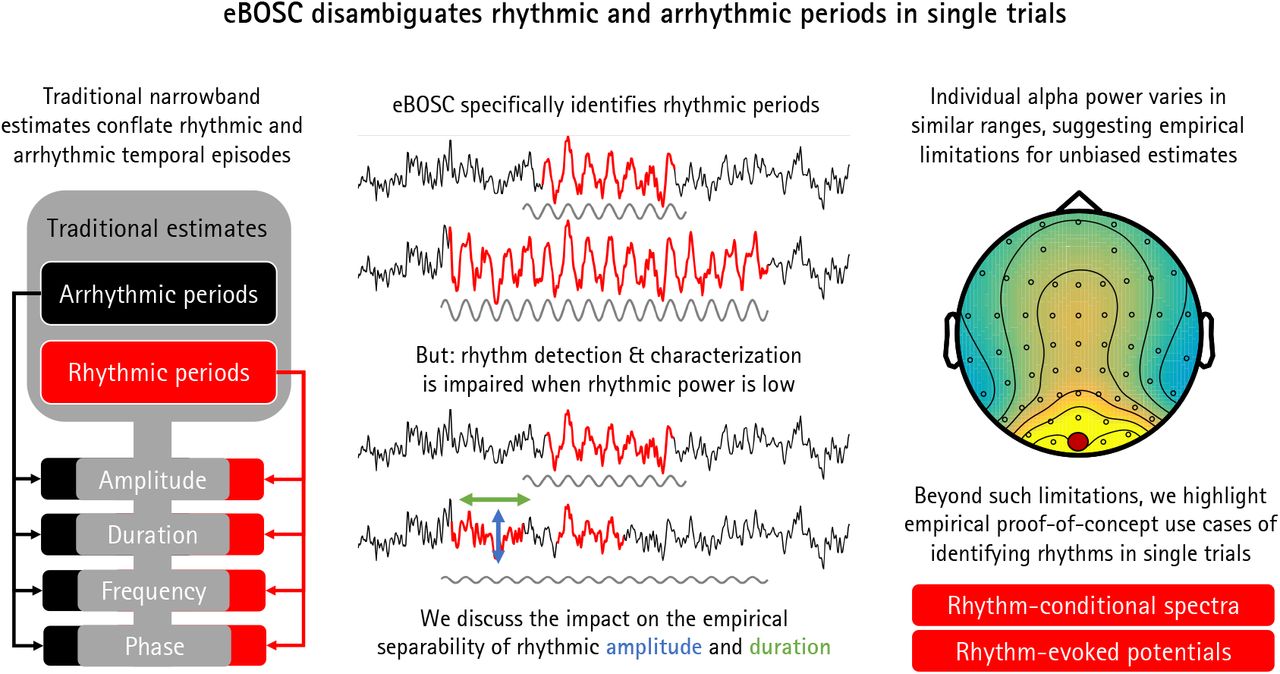
Traditional narrow-band rhythm metrics conflate the power and duration of rhythmic and arrhythmic periods.
We extend a state-of-the-art rhythm detection method (eBOSC) to derive rhythmic episodes in single trials that can disambiguate rhythmic and arrhythmic periods.
Simulations indicate that this can be done with high specificity given sufficient rhythmic power, but with strongly impaired sensitivity when rhythmic power is low.
Empirically, surface EEG recordings exhibit stable inter-individual differences in α-rhythmicity in ranges where simulations suggest a gradual bias, leading to high collinearity between narrow-band and rhythm-specific estimates.
Beyond these limitations, we highlight multiple empirical proof-of-concept benefits of characterizing rhythmic episodes in single trials.
Highlights
1.1 Towards a single-trial characterization of neural rhythms
Episodes of rhythmic neural activity in electrophysiological recordings are of prime interest for research on neural representations and computations across multiple scales of measurement (e.g. Buzsáki, 2006; Wang, 2010). At the macroscopic level, the study of rhythmic neural signals has a long heritage, dating back to Hans Berger’s classic investigations into the Alpha rhythm (Berger, 1938). Since then, advances in recording and processing techniques have facilitated large-scale spectral analysis schemes (e.g. Gross, 2014) that were not available to the pioneers of electrophysiological research, who often depended on the manual analysis of single time series to indicate the presence and magnitude of rhythmic events. Interestingly, improvements in analytic methods still do not capture all of the information that can be extracted by manual inspection. For example, current analysis techniques are largely naïve to the specific temporal presence of rhythms in the continuous recordings, as they often employ windowing of condition- or group-based averages to extract putative rhythm-related characteristics (Cohen, 2014). However, the underlying assumption of stationary, sustained rhythms within the temporal window of interest might not consistently be met (Jones, 2016; Stokes & Spaak, 2016), thus challenging the appropriateness of the averaging model (i.e., the ergodicity assumption (Molenaar & Campbell, 2009)). Furthermore, in certain situations, single-trial characterizations become necessary to derive unbiased individual estimates of neural rhythms (Cohen, 2017). For example, this issue becomes important when asking whether rhythms appear in transient or in sustained form (van Ede, Quinn, Woolrich, & Nobre, 2018), or when only single-shot acquisitions are feasible (i.e., resting state or sleep recordings).
1.2 Duration as a powerful index of rhythmicity
The presence of rhythmicity is a necessary prerequisite for the accurate interpretation of measures of amplitude, power, and phase (Aru et al., 2015; Jones, 2016; Muthukumaraswamy & Singh, 2011). This is exemplified by the bias that arrhythmic periods exert on rhythmic power estimates. Most current time-frequency decomposition methods of neurophysiological signals (such as the electroencephalogram (EEG)) are based on the Fourier transform (Gross, 2014). Following Parceval’s theorem (e.g. Hansen, 2014), the Fast Fourier Transform (FFT) decomposes an arbitrary time series into a sum of sinusoids at different frequencies. Importantly, FFT-derived power estimates do not differentiate between high amplitude transients and low amplitude sustained signals. In the case of FFT power, this is a direct result of the violated assumption of stationarity in the presence of a transient signal. Short-time FFT and wavelet techniques alleviate (but do not eliminate) this problem by analyzing shorter epochs, during which stationarity is more likely to be obtained. However, whenever spectral power is averaged across these episodes, both high-amplitude rhythmic and low-amplitude arrhythmic signal components may once again become intermixed. In the presence of arrhythmic content (often referred to as the “signal background,” or “noise”), this results in a reduced amplitude estimate of the underlying rhythm, the extent of which relates to the duration of the rhythmic episode relative to the length of the analyzed segment (which we will refer to as ‘abundance’) (see Figure 1A). Therefore, integration across epochs that contain a mixture of rhythmic and arrhythmic signals results in an inherent ambiguity between the strength of the rhythmic activity (as indexed by power/amplitude) and its duration (as indexed by the abundance of the rhythmic episode within the segment) (see Figure 3B).

Schematic illustration of rhythm detection. (A) Average amplitude estimates (right) increase with the focus on rhythmic episodes within the averaged time interval. The left plots show simulated time series and the corresponding time-frequency power. Superimposed red traces indicate rhythmic time points. The upper right plot shows the average power spectrum averaged across the entire epoch, the lower plot presents amplitudes averaged exclusively across rhythmic time points. An amplitude gain is observed due to the exclusion of arrhythmic low amplitude time points. (B-E) Comparison of standard and extended BOSC. (B+C) Rhythms were detected based on a power threshold estimated from the arrhythmic background spectrum. Standard BOSC applies a linear fit in log-log space to define the background power, which may overestimate the background at the frequencies of interest in the case of data with large rhythmic peaks. Robust regression following peak removal alleviates this problem. (D) Example of episode detection. White borders circumfuse time frequency points, at which standard BOSC indicated rhythmic content. Red traces represent the continuous rhythmic episodes that result from the extended post-processing. (E) Applied thresholds and detected rhythmic abundance. The black border denotes the duration threshold at each frequency (corresponding to D), i.e., for how long the power threshold needed to be exceeded to count as a rhythmic period. Note that this threshold can be set to zero for a post-hoc characterization of the duration of episodes (see Methods 2.13). The color scaling within the demarcated area indicates the power threshold at each frequency. Abundance corresponds to the relative length of the segment on the same time scale as presented in D. White dots correspond to the standard BOSC measure of rhythmic abundance at each frequency (termed Pepisode). Red lines indicate the abundance measure used here, which is defined as the proportion of sample points at which a rhythmic episode between 8-15 Hz was indicated (shown as red traces in D).
Crucially, the strength and duration of rhythmic activity theoretically differ in their neurophysiological interpretation. Rhythmic power most readily indexes the magnitude of synchronized changes in membrane potentials within a network (Buzsáki, Anastassiou, & Koch, 2012), and is thus related to the size of the participating neural population. The duration of a rhythmic episode, by contrast, tracks how long population synchrony is upheld. Notably, measures of rhythm duration have recently gained interest as they may provide additional information regarding the biophysical mechanisms that give rise to the recorded signals (Peterson & Voytek, 2017; Sherman et al., 2016), for example, by differentiating between transient and sustained rhythmic events (van Ede et al., 2018).
1.3. Single-trial rhythm detection as a methodological challenge
In general, the accurate estimation of process parameters depends on a sufficiently strong signal in the neurophysiological recordings under investigation. Especially for scalp-level M/EEG recordings it remains elusive whether neural rhythms are sufficiently strong to be clearly detected in single trials. Here, a large neural population has to be synchronously active to give rise to potentials that are visible at the scalp surface. This problem intensifies further by signal attenuation through the skull (in the case of EEG) and the superposition of signals from diverse sources of no interest both in- and outside the brain (Lopez da Silva, 2018). In sum, these considerations lead to the proposal that the signal-to-noise ratio (SNR), here operationally defined as the ratio of rhythmic to arrhythmic variance, may fundamentally constrain the accurate characterization of single-trial rhythms.
Following those considerations, we set out to answer the following hypotheses and questions: (1) A precise differentiation between rhythmic and arrhythmic timepoints can disambiguate the strength and the duration of rhythmicity. (2) To what extent does the single-trial rhythm representation in empirical data allow for an accurate estimation of rhythmic strength and duration in the face of variations in the signal-to-noise ratio of rhythmicity? (3) What are the empirical benefits of separating rhythmic (and arrhythmic) duration and power?
Recently, different methods have been proposed to characterize rhythmicity at the single-trial level: the power-based Better OSCillation Detection (BOSC; Caplan, Madsen, Raghavachari, & Kahana, 2001; Whitten, Hughes, Dickson, & Caplan, 2011) and the phase-based lagged coherence index (Fransen, van Ede, & Maris, 2015). Notably, both proposed algorithms make different assumptions regarding the definition of rhythmicity: BOSC assumes that rhythms are defined as spectral peaks that are superimposed on an arrhythmic 1/f background, whereas lagged coherence defines rhythms based on the predictability of phase estimates at a temporal lag that is defined by the rhythm’s period.
Here, we extend the BOSC method (i.e., extended BOSC; eBOSC) to derive rhythmic temporal episodes that can be used to further characterize rhythmicity. Using simulations, we derive rhythm detection benchmarks and probe the boundary conditions for unbiased rhythm indices. Furthermore, we apply the novel eBOSC algorithm to resting- and task-state data from a micro-longitudinal dataset to systematically investigate the feasibility to derive reliable and valid indices of neural rhythmicity from single-trial scalp EEG data. We calculate lagged coherence during the resting state to probe the inter-individual convergence between rhythm definitions. Finally, we showcase eBOSC’s ability to characterize rhythmic and arrhythmic content. We focus on alpha rhythms (~8-15 Hz; defined here based on individual FFT-peaks) due to (a) their high amplitude in human EEG recordings, (b) the previous focus on the alpha band in the rhythm detection literature (Caplan, Bottomley, Kang, & Dixon, 2015; Fransen et al., 2015; Whitten et al., 2011), and (c) their importance for human cognition (Grandy, Werkle-Bergner, Chicherio, Lövdén, et al., 2013a; Klimesch, 2012; Sadaghiani & Kleinschmidt, 2016). We present examples beyond the alpha range to highlight the ability to apply eBOSC in multiple, diverse frequency ranges.
2. Methods
2.1 Study design
Resting state and task data were collected in the context of a larger assessment, consisting of eight sessions in which an adapted Sternberg short-term memory task (Sternberg, 1966) and three additional cognitive tasks were repeatedly administered. Resting state data are from the first session, task data are from sessions one, seven and eight, during which EEG data were acquired. Sessions one through seven were completed on consecutive days (excluding Sundays) with session seven completed seven days after session one by all but one participant (eight days due to a two-day break). Session eight was conducted approximately one week after session seven (M = 7.3 days, SD = 1.4) to estimate the stability of the behavioral practice effects. The reported EEG sessions lasted approximately three and a half to four hours, including approximately one and a half hours of EEG preparation. For further details on the study protocol and results of the behavioural tasks see (Grandy, Lindenberger, & Werkle-Bergner, 2017).
2.2 Participants
The sample contained 32 young adults (mean age = 23.3 years, SD = 2.0, range 19.6 to 26.8 years; 17 women; 28 university students) recruited from the participant database of the Max Planck Institute for Human Development, Berlin, Germany (MPIB). Participants were right-handed, as assessed with a modified version of the Edinburgh Handedness Inventory (Oldfield, 1971), and had normal or corrected-to-normal vision, as assessed with the Freiburg Visual Acuity test (Bach, 1996; 2007). Participants reported to be in good health with no known history of neurological or psychiatric incidences and were paid for their participation (8.08 € per hour, 25.00 € for completing the study within 16 days, and a performance-dependent bonus of 28.00 €; see below). All participants gave written informed consent according to the institutional guidelines of the ethics committee of the MPIB, which approved the study.
2.3 Procedure
Participants were seated at a distance of 80 cm in front of a 60 Hz LCD monitor in an acoustically and electrically shielded chamber. A resting state assessment was conducted prior to the initial performance of the adapted Sternberg task. Two resting state periods were used: the first encompassed a duration of two minutes of continuous eyes open (EO1) and eyes closed (EC1) periods, respectively; the second resting state was comprised of two 80 second runs, totalling 16 repetitions of 5 seconds interleaved eyes open (EO2) – eyes closed (EC2) periods. An auditory beep indicated to the subjects when to open and close their eyes.
Following the resting assessments, participants performed an adapted version of the Sternberg task. Digits were presented in white on a black background and subtended ~2.5° of visual angle in the vertical and ~1.8° of visual angle in the horizontal direction. Stimulus presentation and recording of behavioral responses were controlled with E-Prime 2.0 (Psychology Software Tools, Inc., Pittsburgh, PA, USA). The task design followed the original report (Sternberg, 1966). Participants started each trial by pressing the left and right response key with their respective index fingers to ensure correct finger placement and to enable fast responding. An instruction to blink was given, followed by the sequential presentation of 2, 4 or 6 digits from zero to nine. On each trial, the memory set size (i.e., load) varied randomly between trials, and participants were not informed about the upcoming condition. Also, the single digits constituting a given memory set were randomly selected in each trial. Each stimulus was presented for 200 ms, followed by a fixed 1000 ms blank inter-stimulus interval (ISI). The offset of the last stimulus coincided with the onset of a 3000 ms blank retention interval, which concluded with the presentation of a probe item that was either contained in the presented stimulus set (positive probe) or not (negative probe). Probe presentation lasted 200 ms, followed by a blank screen for 2000 ms, during which the participant’s response was recorded. A beep tone indicated the end of the trial. The task lasted about 50 minutes.
For each combination of load x probe type, 31 trials were conducted, cumulating in 186 trials per session. Combinations were randomly distributed across four blocks (block one: 48 trials; blocks two through four: 46 trials). Summary feedback of the overall mean RT and accuracy within the current session was shown at the end of each block. At the beginning of session one, 24 practice trials were conducted to familiarize participants with the varying set sizes and probe types. To sustain high motivation throughout the study, participants were paid a 28 € bonus if their current session’s mean RT was faster or equal to the overall mean RT during the preceding session, while sustaining accuracy above 90%. Only correct trials were included in the analyses.
2.4 EEG recordings and pre-processing
EEG was continuously recorded from 64 Ag/AgCl electrodes using BrainAmp amplifiers (Brain Products GmbH, Gilching, Germany). Sixty scalp electrodes were arranged within an elastic cap (EASYCAP GmbH, Herrsching, Germany) according to the 10% system (cf. Oostenveld, Fries, Maris, & Schoffelen, 2011) with the ground placed at AFz. To monitor eye movements, two electrodes were placed on the outer canthi (horizontal EOG) and one electrode below the left eye (vertical EOG). During recording, all electrodes were referenced to the right mastoid electrode, while the left mastoid electrode was recorded as an additional channel. Prior to recording, electrode impedances were retained below 5 kΩ. Online, signals were recorded with an analog pass-band of 0.1 to 250 Hz and digitized at a sampling rate of 1 kHz.
Preprocessing and analysis of EEG data were conducted with the FieldTrip toolbox (Oostenveld et al., 2011) and using custom-written MATLAB (The MathWorks Inc., Natick, MA, USA) code. Offline, EEG data were filtered using a 4th order Butterworth filter with a pass-band of 0.5 to 100 Hz, and were linearly detrended. Resting data with interleaved eye closure were epoched relative to the auditory cue to open and close the eyes. An epoch of −2 s to +3 s relative to on- and offsets was chosen to include padding for the analysis. During the eBOSC procedure, three seconds of signal were removed from both edges (see below), resulting in an effective epoch of 4 s duration that excludes evoked components following the cue onset. Continuous eyes open/closed recordings were segmented to the cue on- and offset. For the interleaved data, the first and last trial for each condition were removed, resulting in an effective trial number of 14 trials per condition. For the task data, we analyzed two intervals: an extended interval to assess the overall dynamics of detected rhythmicity and a shorter interval that focused on the retention period. Unless otherwise noted, we refer to the extended interval when presenting task data. For the extended segments, task data were segmented to 21 s epochs ranging from −9 s to +12 s with regard to the onset of the 3 s retention interval for analyses including peri-retention data. For analyses including only the retention phase, data were segmented to −2 s to +3 s around the retention interval. Note that for all analyses, 3 s of signal were removed on each side of the signal during eBOSC detection, effectively removing the evoked cue activity (2 s to account for edge artifacts following wavelet-transformation and 1 s to account for eBOSC’s duration threshold, see section 2.6), except during the extended task interval. Hence, detected segments were restricted to occur from 1s after period onset until period offset, thereby excluding evoked signals. Blink, movement and heart-beat artifacts were identified using Independent Component Analysis (ICA; Bell & Sejnowski, 1995) and removed from the signal. Subsequently, data were downsampled to 250 Hz and all channels were re-referenced to mathematically averaged mastoids. Artifact-contaminated channels (determined across epochs) were automatically detected (a) using the FASTER algorithm (Nolan, Whelan, & Reilly, 2010) and (b) by detecting outliers exceeding three standard deviations of the kurtosis of the distribution of power values in each epoch within low (0.2-2 Hz) or high (30-100 Hz) frequency bands, respectively. Rejected channels were interpolated using spherical splines (Perrin, Pernier, Bertrand, & Echallier, 1989). Subsequently, noisy epochs were likewise excluded based on FASTER and recursive outlier detection, resulting in the rejection of approximately 13% of trials. To prevent trial rejection due to artifacts outside the signal of interest, artifact detection was restricted to epochs that included 2.4 s of additional signal around the on- and offset of the retention interval, corresponding to the longest effective segment that was used in the analyses. A further 2.65% of incorrectly answered trials from the task were subsequently excluded.
2.5 Rhythm-detection using extended BOSC
We applied an extended version of the Better OSCillation detection method (eBOSC; cf. Caplan et al., 2001; Whitten et al., 2011) to automatically separate rhythmic from arrhythmic episodes. The BOSC method reliably identifies rhythms using data-driven thresholds based on theoretical assumptions of the signal characteristics. Briefly, the method defines rhythms as time points during which wavelet-derived power at a particular frequency exceeds a power threshold based on an estimate of the arrhythmic signal background. The theoretical duration threshold defines a minimum duration of cycles this power threshold has to be exceeded to exclude high amplitude transients. Previous applications of the BOSC method focused on the analysis of resting-state data or long data epochs, where reliable detection has been established regardless of specific parameter setups (Caplan et al., 2001; 2015; Whitten et al., 2011). We introduce the following adaptations here (for details see section 2.6, Figures 1 & 2): (1) we remove the spectral alpha peak and use robust regression to establish power thresholds; (2) we combine detected time points into continuous rhythmic episodes and (3) we reduce the impact of wavelet convolution on abundance estimates. We benchmarked the algorithm and compared it to standard BOSC using simulations (see section 2.8).

Example of eBOSC’s post-processing routines to derive sparse continuous rhythmic ‘episodes’. (A) Simulated signal containing 1/f noise and superimposed 10 Hz rhythmicity. (B) 10 Hz rhythmic signal only. (C) Traditional output of BOSC detection: a binary matrix indicates time-frequency points that adhere to power and duration thresholds (in yellow). These matrices are used to calculate Pepisode. (D) First step of eBOSC’s post-processing: the detected matrix is ‘sparsified’ in the spectral dimension to create continuous rhythmic episodes. (E) Second step of eBOSC’s post-processing: each episode is temporally corrected for the temporal wavelet convolution by estimating the bias of each time point on adjacent time points (here exemplified for select time points via red traces). Only time points that exceed the bias estimated from surrounding time points are retained. (F) Example of final episode trace. The black line indicates the time points that were retained, whereas the red segments were removed during step E. The final episode output is then characterized according to e.g., mean frequency, duration and amplitude, whereas the time points of rhythmicity can for example be used to define rhythm-conditional spectra. These episodes are used to calculate abundance.
2.6 Specifics of rhythm-detection using extended BOSC
Rhythmic events were detected within subjects for each channel and condition. Time-frequency transformation of single trials was performed using 6-cycle Morlet wavelets (Grossmann & Morlet, 1985) with 49 logarithmically-spaced center frequencies ranging from 1 to 64 Hz. Following the wavelet transform, 2 s were removed at each segment’s borders to exclude edge artefacts. To estimate the background spectrum, the time-frequency spectra from all trials were temporally concatenated within condition and channel and log-transformed, followed by temporal averaging. For eyes-closed and eyes-open resting states, both continuous and interleaved exemplars were included in the background estimation for the respective conditions. The resulting power spectrum was fit linearly in log(frequency)-log(power) coordinates using a robust regression, with the underlying assumption that the EEG background spectrum is characterized by colored noise of the form A*f^(−α) (Buzsáki & Mizuseki, 2014; He, Zempel, Snyder, & Raichle, 2010; Linkenkaer-Hansen, Nikouline, Palva, & Ilmoniemi, 2001). A robust regression with bisquare weighting (e.g. Holland & Welsch, 2007) was chosen to improve the linear fit of the background spectrum (cf. Haller et al., 2018), which is characterized by frequency peaks in the alpha range for almost all subjects (Supplementary Figure 2). In contrast to ordinary least squares regression, robust regression iteratively down-weights outliers (in this case spectral peaks) from the linear background fit. To improve the definition of rhythmic power estimates as outliers during the robust regression, power estimates within the wavelet pass-band around the individual alpha peak frequency were removed prior to fitting1. The passband of the wavelet (e.g. Linkenkaer-Hansen et al., 2001) was calculated as
 in which IAF denotes the individual alpha peak frequency and WL refers to wavelet length (here, six cycles in the main analysis). IAF was determined based on the peak magnitude within the 8-15 Hz average spectrum for each channel and condition (Grandy, Werkle-Bergner, Chicherio, Schmiedek, et al., 2013b). This ensures that the maximum spectral deflection is removed across subjects, even in cases where no or multiple peaks are present2. This procedure effectively removes a bias of the prevalent alpha peak on the arrhythmic background estimate (see Figure 1B and C & Figure 4C). The power threshold for rhythmicity at each frequency was set at the 95th percentile of a χ2(2)-distribution of power values, centered on the linearly fitted estimate of background power at the respective frequency (for details see Whitten et al., 2011). This essentially implements a significance test of single-trial power against arrhythmic background power. A three-cycle threshold was used as the duration threshold to exclude transients, unless indicated otherwise (see section 2.13). The conjunctive power and duration criteria produce a binary matrix of ‘detected’ rhythmicity for each time-frequency point (see Figure 2C). To account for the duration criterion, 1000 ms were discarded from each edge of this ‘detected’ matrix.
The original BOSC algorithm was further extended to define rhythmic events as continuous temporal episodes that allow for an event-wise assessment of rhythm characteristics (e.g. duration). The following steps were applied to the binary matrix of ‘detected’ single-trial rhythmicity to derive such sparse and continuous episodes. First, to account for the spectral extension of the wavelet, we selected time-frequency points with maximal power within the wavelet’s spectral smoothing range (i.e. the pass-band of the wavelet;  ; see Formula 1). That is, at each time point, we selected the frequency with the highest indicated rhythmicity within each frequency’s pass-band. This served to exclude super-threshold timepoints that may be accounted for by spectral smoothing of a rhythm at an adjacent frequency. Note that this effectively creates a new frequency resolution for the resulting rhythmic episodes, thus requiring sufficient spectral resolution (defined by the wavelet’s pass-band) to differentiate simultaneous rhythms occurring at close frequencies. Finally, continuous rhythmic episodes were formed by temporally connecting extracted time points, while allowing for moment-to-moment frequency transitions (i.e. within-episode frequency non-stationarities; Atallah & Scanziani, 2009) (for a single-trial illustration see Figures 1D and 2D).
In addition to the spectral extension of the wavelet, the choice of wavelet parameter also affects the extent of temporal smoothing, which may bias rhythmic duration estimates. To decrease such temporal bias, we compared observed rhythmic amplitudes at each time point within each rhythmic episode with those expected by smoothing adjacent amplitudes using the wavelet (Figure 2E). By retaining only those time points where amplitudes exceeded the smoothing-based expectations, we removed supra-threshold time points that can be explained by temporal smoothing of nearby rhythms (e.g., ‘ramping’ up and down signals). In more detail, we simulated the positive cycle of a sine wave at each frequency, zero-shouldered each edge and performed (6-cycle) wavelet convolution. The resulting amplitude estimates at the zero-padded time points reflect the temporal smoothing bias of the wavelet on adjacent arrhythmic time points. This bias is maximal (BiasMax) at the time point immediately adjacent to the rhythmic on-/offset and decreases with temporal distance to the rhythm. Within each rhythmic episode, the ‘convolution bias’ of a time-frequency (TF) point’s amplitude on surrounding points was estimated by scaling the points’ amplitude by the modelled temporal smoothing bias.

Subscripts F and T denote frequency and time within each episode, respectively. BiasVector is a vector with the length of the current episode (L) that is centered around the current TF-point. It contains the wavelet’s symmetric convolution bias around BiasMax. Note that both BiasVector and BiasMax respect the possible frequency variations within an episode (i.e., they reflect the differences in convolution bias between frequencies). The estimated wavelet bias was then scaled to the amplitude of the rhythmic signal at the current TF-point. PT refers to the condition- and frequency-specific power threshold applied during rhythm detection. We subtracted the power threshold to remove arrhythmic contributions. This effectively sensitizes the algorithm to near-threshold values, rendering them more likely to be excluded. Finally, time points with lower amplitudes than expected by the convolution model were removed and new rhythmic episodes were created (Figure 2F). The resulting episodes were again checked for adhering to the duration threshold.
As an alternative to the temporal wavelet correction based on the wavelet’s simulated maximum bias (‘MaxBias’; as described above), we investigated the feasibility of using the wavelet’s full-width half maximum (‘FWHM’) as a criterion. Within each continuous episode and for each “rhythmic” sample point, 6-cycle wavelets at the frequency of the neighbouring points were created and scaled to the point’s amplitude. We then used the amplitude of these wavelets at the FWHM as a threshold for rhythmic amplitudes. That is, points within a rhythmic episodes that had amplitudes below those of the scaled wavelets were defined as arrhythmic. The resulting continuous episodes were again required to pass the duration threshold. As the FWHM approach indicated decreased specificity of rhythm detection in the simulations (Supplementary Figure 1) we used the ‘MaxBias’ method for our analyses.
Furthermore, we considered a variant where total amplitude values were used (vs. supra-threshold amplitudes) as the basis for the temporal wavelet correction. Our results suggest that using supra-threshold power values leads to a more specific detection at the cost of sensitivity (Supplementary Figure 1). Crucially, this eliminated false alarms and abundance overestimation, thus rendering the method highly specific to the occurrence of rhythmicity. As we regard this as a beneficial feature, we used supra-threshold amplitudes as the basis for the temporal wavelet correction throughout the manuscript.
2.7 Definition of abundance, rhythmic probability and amplitude metrics
A central goal of rhythm detection is to disambiguate rhythmic power and duration (Figure 3). For this purpose, eBOSC provides multiple indices. We describe the different indices for the example case of alpha rhythms. Please note that eBOSC can be applied in a similar fashion to any other frequency range. The abundance of alpha rhythms denotes the duration of rhythmic episodes with a mean frequency in the alpha range (8 to 15 Hz), relative to the duration of the analyzed segment. This frequency range was motivated by clear peaks within this range in individual resting state spectra (Supplementary Figure 2). Note that abundance is closely related to standard BOSC’s Pepisode metric (Whitten et al., 2011), with the difference that abundance refers to the duration of the continuous rhythmic episodes and not the ‘raw’ detected rhythmicity of BOSC (cf. Figure 2C and D). We further define rhythmic probability as the across trials probability to observe a detected rhythmic episode within the alpha frequency range at a given point in time. It is therefore the within-time, across-trial equivalent of abundance.

eBOSC disambiguates the magnitude and duration of rhythmic episodes. (A) Schema of different amplitude metrics. (B) Rhythm-detection disambiguates rhythmic amplitude and duration. Overall amplitudes represent a mixture of rhythmic power and duration. In the absence of noise (upper row), eBOSC perfectly orthogonalizes rhythmic amplitude from abundance. Superimposed noise leads to an imperfect separation of the two metrics (lower row). The duration of rhythmicity is similarly indicated by abundance and the overlap between rhythmic and overall amplitudes. This can be seen by comparing the two rightmost plots in each row.
As a result of rhythm detection, the magnitude of spectral events can be described using multiple metrics (see Figure 3A for a schematic). The standard measure of window-averaged amplitudes, overall amplitudes were computed by averaging across the entire segment at its alpha peak frequency. In contrast, rhythmic amplitudes correspond to the amplitude estimates during detected rhythmic episodes. If no alpha episode was indicated, abundance was set to zero, and amplitude was set to missing. Unless indicated otherwise, both amplitude measures were normalized by subtracting the amplitude estimate of the fitted background spectrum. This step represents a parameterization of rhythmic power (cf. Haller et al., 2018) and is conceptually similar to baseline normalization, without requiring an explicit baseline segment. This highlights a further advantage of rhythm-detection procedures like (e)BOSC. In addition, we calculated an overall signal-to-noise ratio (SNR) as the ratio of the overall amplitude to the background amplitude:  . In addition, we defined rhythmic SNR as the background-normalized rhythmic amplitude as a proxy for the rhythmic representation:
  . Unless stated differently, subject-, and condition-specific amplitude and abundance values were averaged within and across trials, and across posterior-occipital channels (P7, P5, P3, P1, Pz, P2, P4, P6, P8, PO7, PO3, POz, PO4, PO8, O1, Oz, O2), in which alpha power was maximal (Figure 5A, Figure 11).
2.8 eBOSC validation via alpha rhythm simulations
To assess eBOSC’s detection performance, we simulated 10 Hz sine waves with varying amplitudes (0, 2, 4, 6, 8, 12, 16, 24 [a.u.]) and durations (2, 4, 8, 16, 32, 64, 128, 200 [cycles]) that were symmetrically centred within random 1/f-filtered white noise signals (20 s; 250 Hz sampling rate). Amplitudes were scaled relative to the power of the 8-12 Hz 6th order Butterworth-filtered background signal in each trial to approximate SNRs. To ensure comparability with the empirical analyses, we computed overall SNR analogously to the empirical data, which tended to be lower than the target SNR. We chose the maximum across simulated durations as an upper bound (i.e., conservative estimate) on overall SNR. For each amplitude-duration combination we simulated 500 “trials”. We assessed three different detection pipelines regarding their detection efficacy: the standard BOSC algorithm (i.e., linear background fit incorporating the entire frequency range with no post-editing of the detected matrix); the eBOSC method using wavelet correction by simulating the maximum bias introduced by the wavelet (“MaxBias); and the eBOSC method using the full-width-at-half-maximum amplitude for convolution correction (“FWHM”). The background was estimated separately for each amplitude-duration combination. 500 edge points were removed bilaterally following wavelet estimation, 250 additional samples were removed bilaterally following BOSC detection to account for the duration threshold, effectively retaining 14 s of simulated signal.
Detection efficacy was indexed by signal detection criteria regarding the identification of rhythmic time points between 8 and 12 Hz (i.e., hits = simulated and detected points; false alarms = detected, but not simulated points). These measures are presented as ratios to the full amount of possible points within each category (e.g., hit rate = hits/all simulated time points). For the eBOSC pipelines, abundance was calculated identically to the analyses of empirical data. As no consecutive episodes (cf. Pepisode and abundance) are available in standard BOSC, abundance was defined as the relative amount of time points with detected rhythmicity between 8 to 12 Hz.
A separate simulation aimed at establishing the ability to accurately recover amplitudes. For this purpose, we simulated a whole-trial alpha signal (i.e., duration = 1) and a quarter-trial alpha signal (duration = .25) with a larger range of amplitudes (1:16 [a.u.]) and performed otherwise identical procedures as described above. To assess eBOSC’s ability to disambiguate power and duration (Figure 3B), we additionally performed simulations in the absence of noise across a larger range of simulated amplitudes and durations.
A major change in eBOSC compared to standard BOSC is the exclusion of the rhythmic peak prior to estimating the background. To investigate to what extent the two methods induce a bias between rhythmicity and the estimated background magnitude (for a schematic see Figure 1C and D), we calculated Pearson correlations between the overall amplitude and the estimated background amplitude across all levels of simulated amplitudes and durations (Figure 4C).

Rhythm detection performance of standard and extended BOSC in simulations. (A) Signal detection properties of the two algorithms. For short simulated rhythmicity, abundance is overestimated by standard BOSC, but not eBOSC, whereas eBOSC underestimates the duration of prolonged rhythmicity at low SNRs (A1). Extended BOSC has decreased sensitivity (A2), but higher specificity (A3) compared with extended BOSC. Note that for simulated zero alpha amplitude, all sample points constitute potential false alarms, while by definition no sample point constitutes a potential hit. (B) Amplitude and abundance estimates for signals with sustained (left) and short rhythmicity (right). Black dots indicate reference estimates for a pure sine wave without noise, coloured dots indicate the respective estimates for data with the 1/f background. [Note that the reference estimates were interpolated at the empirical abundance of the 1/f data. Grey dots indicate the perfect abundance estimates in the absence of background noise.] When rhythms are sustained (left), impaired rhythm detection at low SNRs causes an overestimation of the rhythmic amplitude. At low rhythmic duration (right), this deficit is outweighed by the severe bias of arrhythmic duration on overall amplitude estimates (e.g., Figure 13). Simulated amplitudes (and corresponding empirical SNRs in brackets) are shown on the right. Vertical lines indicate the simulated rhythmic duration. (C) eBOSC successfully reduces the bias of the rhythmic peak on the estimation of the background amplitude. In comparison, standard BOSC induces a strong coupling between the peak magnitude and the background estimate. (D) eBOSC indicates abundance more accurately than standard BOSC at high amplitudes (i.e., high SNR; see also A1). The leftward shift indicates a decrease in sensitivity. Horizontal lines indicate different levels of simulated duration. Dots are single-trial estimates across levels of simulated amplitude and duration. (E) Standard BOSC and eBOSC induce trial-wise correlations between amplitude and abundance. eBOSC exhibits reduced trial-by-trial coupling at higher SNR compared to standard BOSC. Values are r-to-z-transformed correlation coefficients.
As the empirical data suggested a trial-wise association between amplitude and abundance estimates also at high levels of signal-to-noise ratios (Figure 8), we investigated whether such associations were also present in the simulations. For each pair of simulated amplitude and duration, we calculated Pearson correlations between the overall amplitude and abundance across single trials. Note that due to the stationarity of simulated duration, trial-by-trial fluctuations indicate the bias under fluctuations of the noise background (as amplitudes were scaled to the background in each trial). For each cell, we performed Fisher’s r-to-z transform to account for unequal trial sizes due to missing amplitude/abundance estimates (e.g. when no episodes are detected).
2.9 Calculation of phase-based lagged coherence
To investigate the convergence between the power-based duration estimate (abundance) and a phase-based alternative, we calculated lagged coherence at 40 linearly scaled frequencies in the range of 1 to 40 Hz for each resting-state condition. Lagged coherence assesses the consistency of phase clustering at a single sensor for a chosen cycle lag (see Fransen et al., 2015 for formulas). Instantaneous power and phase were estimated via 3-cycle wavelets. Data were segmented to be identical to eBOSC’s effective interval (i.e., same removal of signal shoulders as described above). In reference to the duration threshold for power-based rhythmicity, we calculated the averaged lagged coherence using two adjacent epochs à three cycles. We computed an index of alpha rhythmicity by averaging values across epochs and posterior-occipital channels, finally extracting the value at the maximum lagged coherence peak in the 8 to 15 Hz range.
2.10 Dynamics of rhythmic probability and rhythmic power during task performance
To investigate the detection properties in the task data, we analysed the temporal dynamics of rhythmic probability and power in the alpha band. We created time-frequency representations as described in section 2.6 and extracted the IAF power time series, separately for each person, condition, channel and trial. At the single-trial level, values were allocated to rhythmic vs. arrhythmic time points according to whether a rhythmic episode with mean frequency in the respective range was indicated by eBOSC (Figure 2B; Figure 3C). These time series were averaged within subject to create individual averages of rhythm dynamics. Subsequently, we z-scored the power time series to accentuate signal dynamics and attenuate between-subject power differences. To highlight global dynamics, these time series were further averaged within- and between-subjects. Figure captions indicate which average was used.
2.11 Rhythmic frequency variability during rest
As an exemplary characteristic of rhythmicity, we assessed the stability of IAF estimates by considering the variability across trials of the task as a function of indicated rhythmicity. Trial-wise rhythmic IAF variability (Figure 10A) was calculated as the standard deviation of the mean frequency of alpha episodes (8-15 Hz). That is, for each trial, we averaged the estimated mean frequency of rhythmic episodes within that trial and computed the standard deviation across trials. Whole-trial IAF variability (Figure 10B) was similarly calculated as the standard deviation of the IAF, with single-trial IAF defined as the frequency with the largest peak magnitude between 8-15 Hz, averaged across the whole trial, i.e., encompassing segments both designated as rhythmic and arrhythmic. Finally, we compared the empirical variability with that observed in simulations (see section 2.8).
2.12 Rhythm-conditional spectra and abundance for multiple canonical frequencies
To assess the general feasibility of rhythm detection outside the alpha range, we analysed the retention interval of the adapted Sternberg task, where the occurrence of theta, alpha and beta rhythms has been reported in previous studies (Brookes et al., 2011; Jensen, Gelfand, Kounios, & Lisman, 2002; Jokisch & Jensen, 2007; Lundqvist et al., 2016; Raghavachari et al., 2001; Tuladhar et al., 2007). For this purpose, we re-segmented the data to cover the final 2 s of the retention interval +-3 s of edge signal that was removed during the eBOSC procedure. We performed eBOSC rhythm detection with otherwise identical parameters to those described in section 2.6. We then calculated spectra across those time points where rhythmic episodes with a mean frequency in the range of interest were indicated, separately for four frequency ranges: 3-8 Hz (theta), 8-15 Hz (alpha), 15-25 Hz (beta) and 25-64 Hz (gamma). We subtracted spectra across the remaining arrhythmic time-points for each range from these ‘rhythm-conditional’ spectra to derive the spectra that are unique to those time points with rhythmic occurrence in the band of interest.
For the corresponding topographic representations, we calculated the abundance metric as described in section 2.7 for the apparent peak frequency ranges.
2.13 Post-hoc characterization of sustained rhythms vs. transients
Instead of exclusively relying on a fixed a priori duration threshold as done in previous applications, eBOSC’s continuous ‘rhythmic episodes’ also allow for a post-hoc separation of rhythms and transients based on the duration of identified rhythmic episodes. This is afforded by our extended post-processing that results in a more specific identification of rhythmic episodes (see Figure 4) and an estimated length for each episode. For this analysis (Figure 14), we set the a priori duration threshold to zero and separated the resulting episodes post-hoc based on their duration (shorter vs. longer than 3 cycles) at their mean frequency. That is, any episode crossing the amplitude threshold was retained and episodes were sorted by their ‘transient’ or sustained appearance afterwards. We conducted this analysis in the extended task data to highlight the temporal dynamics of rhythmic and transient events.
Similarly, the temporal specificity of rhythmic episodes allow the assessment of ‘rhythm-evoked’ effects in the temporal or spectral domain. Here, we showcase the rhythm-evoked changes in the same frequency band to indicate the temporal specificity of the indicated rhythmic periods (Figure 15). For this purpose, we calculated time-frequency representations using 6-cycle wavelets and extracted power in the theta (3-8 Hz), alpha (8-15 Hz), beta (15-25 Hz) and gamma-band (25-64 Hz) in 2.4 s periods centred on the on- and offset of indicated rhythmic periods in the respective band. Separate TFRs were calculated for the detected episodes in each channel, followed by averaging across episodes and channels. Finally, we z-transformed the individual averages to highlight the consistency across subjects.
3. Results
3.1. Extended BOSC (eBOSC) increases specificity of rhythm-detection
We extended the BOSC rhythm detection method to characterize rhythmicity at the single-trial level by creating continuous ‘rhythmic episodes’ (see Figure 1 & 2). A central goal of this approach is the disambiguation of rhythmic power and duration (see Figure 3). In situations without background noise, this can be achieved perfectly. However, the addition of 1/f noise leads to a partial coupling of the two parameters. As we introduced changes to the original method, we compared the detection properties of the standard and the extended (eBOSC) pipeline by simulating varying levels of rhythm magnitude and duration.
Considering the sensitivity and specificity of detection, both pipelines performed adequately at high levels of SNR with high hit and low false alarm rates (Figure 4A). However, we observed important differences between the algorithms. While standard BOSC showed perfect sensitivity above overall SNRs of ~4, specificity was lower than for eBOSC as indicated by higher false alarm rates (grand averages: .160 for standard BOSC; .015 for eBOSC). This specificity increase is observed across simulation parameters, suggesting a general abundance overestimation by standard BOSC (see also Figure 4D). In addition, standard BOSC did not show a reduced detection of transient rhythms below the duration threshold of three cycles, whereas hit rates for those transients were clearly reduced in eBOSC (Figure 4A2). This suggests that wavelet-convolution extended the effective duration of transient rhythmic episodes, resulting in an exceedance of the temporal threshold. In contrast, by creating explicit rhythmic episodes and reducing convolution effects, eBOSC more strictly adheres to the specified target duration. However, there was also a notable reduction in sensitivity for rhythms just above the duration threshold, suggesting a sensitivity-specificity trade-off (Figure 4A2). In addition to decreasing false alarms, eBOSC also more accurately estimated the duration of rhythmicity (Figure 4A1), although an underestimation of abundance persisted (and was increased) at low SNRs. In sum, while eBOSC improves the specificity of identifying rhythmic content, there are also noticeable decrements in sensitivity (grand averages: .909 for standard BOSC; .614 for eBOSC), especially at low SNRs. Notably, while sensitivity remains an issue, the high specificity of detection suggests that the estimated rhythmic abundance serves as a lower bound on the actual duration of rhythmicity.
In a second set of simulations, we considered eBOSC’s potential to accurately estimate rhythmic amplitudes. As expected, in signals with stationary rhythms (duration = 1), the overall amplitude most accurately represented the simulated amplitude (Figure 4B left), as any methods-induced underestimation would introduce inaccuracies. Hence, at lower SNRs, underestimation of rhythmic content resulted in an overestimation of rhythmic power, as some low-amplitude time points were incorrectly excluded prior to averaging. At those low SNRs, subtraction of the background estimate (cf. baseline normalization) alleviates this overestimation. The general impairment at low SNRs is however outweighed by the advantage of rhythm-specific amplitude estimates in time series where rhythmic duration is low and thus arrhythmicity is prevalent (Figure 4B right). Here, rhythm-specific estimates accurately track simulated amplitudes, whereas a strong underestimation is observed for unspecific power indices. We again observed an underestimation of rhythmic duration with decreasing amplitudes (as in Figure 4A1).
An adaptation of the eBOSC method is the exclusion of the rhythmic alpha peak prior to fitting the arrhythmic background. This serves to reduce a potential bias of rhythmic content on the estimation of the arrhythmic content (see Figure 1C for a schematic). Our simulations indeed indicate a bias of the spectral peak amplitude on the background estimate in the standard BOSC algorithm, which is substantially reduced in eBOSC (Figure 4C).
To gain a visual representation of duration estimation performance, we plotted abundance against amplitude estimates across all simulated trials, regardless of simulation parameters (Figure 4D). This reveals multiple modes of abundance at high levels of amplitude, which in the eBOSC case more closely track the simulated duration. This further visualizes the decreased error in abundance estimates, especially at high SNRs (e.g., Figure 4A), while an observed rightward shift towards higher amplitudes indicated the more pronounced underestimation of rhythmicity when SNRs are low.
Finally, we investigated the trial-wise association between amplitude and duration estimate based on the observed coupling in empirical data (see Figure 8). Our simulations suggest that both standard BOSC and eBOSC can induce spurious positive correlations between amplitude and abundance estimates, which are most pronounced at low levels of SNR (Figure 4E). Notably, these associations are strongly reduced in eBOSC, especially when rhythmic power is high. While this suggests a remaining methods-induced association between the two parameters, it also indicates that eBOSC provides a better separation between the two (here independently simulated) parameters.
In sum, our simulations suggest that eBOSC specifically separates rhythmic and arrhythmic time points in simulated data at the expense of decreased sensitivity, especially when SNR is low. However, the increase in specificity is accompanied by an increased accuracy of duration estimates at high SNR, theoretically allowing a more precise investigation of rhythmic duration.
3.2 eBOSC detects single-trial alpha rhythms during rest and task states
While the simulations provide a gold standard to assess detection performance, we further probed eBOSC’s detection performance in empirical data from resting and task states to investigate the practical feasibility and utility of rhythm detection. As the ground truth in real data is unknown, we evaluated detection performance by contrasting metrics from detected and undetected timepoints regarding their topography and time course.
Individual power spectra showed clear rhythmic alpha peaks for every participant during eyes closed rest and for most subjects during eyes open rest and the task retention period, indicating the general presence of alpha rhythms during the analysed states (Supplementary Figure 2). In line with a putative source in visual cortex, alpha abundance was highest over parieto-occipital channels during the resting state (Figure 5A) and during the WM retention period (Figure 11). As expected, rhythmic time-points exhibited increased alpha power compared with arrhythmic time points (Figure 5A). In addition, alpha power and abundance underwent state modulations. As one of the earliest findings in cognitive electrophysiology (Berger, 1938), alpha amplitudes increase in magnitude upon eye closure. Here, eye closure was reflected by a joint shift towards higher amplitudes and durations for almost all participants (Figure 5B), suggesting that both parameters similarly reflected the state shift.

Rhythmic abundance and amplitude during rest. (A) eBOSC identifies high occipital alpha abundance and rhythmic amplitude especially during the Eyes Closed resting state. (B) Eye closure modulates both rhythmic amplitude and abundance on an individual level. Arrows indicate the direction and magnitude of parameter change upon eye closure for each subject. Red arrows indicate data during continuous eyes closed/eyes open intervals, blue arrows represent data from the interleaved acquisition. Thick arrows indicate the group average.
The temporal dynamics of indicated rhythmicity are another characteristic of interest, which we assessed by considering the rhythmic probability across trials at each time point. While such an investigation is difficult for induced rhythmicity during rest, evoked rhythmicity offers an optimal test case due to its systematic temporal deployment. For this reason, we analysed task recordings with stereotypic design-locked alpha power dynamics at encoding, retention and probe presentation (Figure 6AB). At the average level, rhythmic probability closely tracked power dynamics (Figure 6A) and time points designated as rhythmic exhibited pronounced alpha power compared with those labelled arrhythmic (6A3 vs. 6A4; 6A5 vs. 6A6). While rhythm-specific dynamics were closely capturing standard power trajectories, we observed a dissociation concerning arrhythmic power. Here, we observed transient increases during stimulus onsets that were absent from either abundance or rhythmic power (Figure 6A6). This suggests an increase in high-power transients that were excluded due to the 3 cycle duration threshold. Indeed, an increase in transient events was observed without an a priori duration threshold (see Figure 14). In sum, these results suggest an accurate detection at the average level. However, we also observed large inter-individual variability in detected rhythmicity (Figure 6A2). Such result is consistent with the prevalence of shorter rhythmicity or a general absence of rhythmic content. To resolve this ambiguity, we investigated detection in single trials.

Characterization of detected single-trial rhythmicity during task performance. (A) Average evoked alpha power and rhythmic probability at posterior-occipital channels. (A1-A4) Individual dynamics of power and rhythmicity. (A5) Rhythmic power at IAF (blue) and rhythm probability (red) exhibit stereotypic temporal dynamics during encoding (red bars), retention (0 to 3 s) and retrieval (black bars). (A6) While arrhythmic power exhibits similar temporal dynamics, it is strongly reduced in power (see scales in A5 and A6). The arrhythmic power dynamics are characterized by additional transient increases following stimulus presentations (blue vs. red traces between vertical bars; cf., A6). Data are from the first session and the high load condition. (B) Task-related alpha dynamics are captured by eBOSC at the single-trial level. Each box displays individual trial-wise z-standardized IAF alpha power, separately for rhythmic (left) and non-rhythmic (right) time points. While rhythmic time points (left) exhibit clear single-trial power increases that are locked to the task design, arrhythmic time points (right) do not show evoked task dynamics that separate them from the background, hence suggesting an accurate rejection of rhythmicity. The subplots’ frame colour indicates the subjects’ raw power maximum (i.e., the data scaling). Data are from channel O2 during the first session across load conditions. (C) Individual abundance estimates are stable across sessions. Data were averaged across posterior-occipital channels and high (i.e., 6) item load trials.
At the single-trial level, rhythmicity was indicated for periods with visibly elevated alpha power with strong task-locking (Figure 6B left). Conversely, arrhythmicity was indicated for time points with low alpha power and little structured dynamics (Figure 6B right). However, strong inter-individual differences were apparent, with little detected rhythmicity when global alpha power was low (Figure 6B bottom; plots are sorted by descending power as indicated by the frame colour of the depicted subjects and scaled using z-scores to account for global power differences). Crucially, those subjects’ single-trial power dynamics did not present a clear temporal structure, suggesting a prevalence of noise and therefore a correct rejection of rhythmicity.
Notably, individual rhythmicity estimates were stable across multiple sessions (Figure 6C), suggesting that they are indicative of trait-like characteristics rather than idiosyncratic measurement noise (Grandy et al., 2013). Note that it is unlikely that such detection differences are primarily due to misfits of the background spectrum. Simulations suggest that compared to the linear background fit that is implemented in standard BOSC, the robust fit with alpha peak removal successfully removes the bias of rhythmic alpha power on background estimates (Figure 4C), while individual power thresholds indicate a successful exclusion of the alpha peak (Supplementary Figure 2).
In sum, these results suggest that eBOSC successfully separates rhythmic and arrhythmic episodes in empirical data, both at the group and individual level. However, they also suggest prevalent and stable differences in single-trial rhythmicity in the alpha band.
3.3 Rhythmic SNR constrains indicated rhythmicity and rhythm-related metrics
While the empirical results suggest a successful separation of rhythmic and arrhythmic content at the single-trial level, we also observed strong (and stable) inter-individual differences in alpha-abundance. This may imply actual differences in the duration of rhythmic engagement (as indicated in Figure 6B). However, we also observed a severe underestimation of abundance as a function of the overall signal-to-noise ratio (SNR) in simulations (Figure 4), thus leading to the question whether empirical data fell into similar ranges where an underestimation was likely. To answer this question, we calculated the individual overall SNR during the resting state. We indeed observed that many overall SNRs were in the range, where simulations with a stationary alpha rhythm suggested an underestimation of abundance (blue line in Figure 7A. The black line indicates simulation-based estimates for stationary alpha rhythms at different overall SNR levels; see section 2.8). Moreover, the coupling of individual SNR and abundance values took on a deterministic shape in this range, whereas the association was reduced in ranges where simulations suggest sufficient SNR for unbiased abundance estimates (orange line in Figure 7A). As overall SNR is influenced by the duration of arrhythmic signal, rhythmic SNR may serve as an even better predictor of abundance due to its specific relation to rhythmic episodes (Figure 3). In line with this consideration, rhythmic SNR exhibited a strong linear relationship to abundance (Figure 7B). Importantly, the background estimate was not consistently related to abundance (Figure 7C), emphasizing that it is the ‘signal’ and not the ‘noise’ component of SNR that determines detection. Similar observations were made in the task data during the retention phase (Supplementary Figure 3), suggesting that this association reflects a general link between the magnitude of the spectral peak and duration estimates. The joint analysis of simulated and empirical data thus question the accuracy of individual duration estimates, especially at low SNRs, due to the dependence of unbiased estimates on sufficient rhythmic power.

Inter-individual alpha abundance is strongly associated with rhythmic, but not arrhythmic power and may be underestimated at low rhythmic SNR. (A) Individual abundance estimates are strongly related to the overall SNR of the spectral alpha peak. This relationship is also observed when only considering individual data within the SNR range for which simulation analyses indicated an unbiased abundance estimation. The black line indicates interpolated estimates from simulation analyses with a sustained rhythm (i.e., duration = 1; see Figure 4B left). Hence, it indicates a lower bound for the abundance underestimation that occurs at low SNRs, with notable overlap with the empirical estimates in the same SNR range. (B) The effective rhythmic signal can be conceptualized as the background-normalized rhythmic amplitude above the background estimate (rhythmic SNR). This proxy for signal clarity is inter-individually linked to abundance estimates. (C) Background estimates are not consistently related to abundance. This implies that the relationship between amplitude and abundance is mainly driven by the signal, but not background amplitude (i.e., the effective signal ‘clarity’) and that associations do not arise from a misfit of the background. (D) Rhythmicity estimates translate between power- and phase-based definition of rhythmicity. This indicates that the BOSC-detected rhythmic spectral peak above the 1/f spectrum contains the rhythmic information that is captured by phase-based duration estimates. All data are from the resting state.
As eBOSC defines single-trial power deviations from a stationary power threshold as a criterion for rhythmicity, it remains unclear whether this association is exclusive to such a ‘power thresholding’-approach or whether it constitutes a more general feature of single-trial rhythmicity. To probe this question, we calculated a phase-based measure of rhythmicity, termed ‘lagged coherence’ (Fransen et al., 2015), which assesses the stability of phase clustering at a single sensor for a chosen cycle lag. Here, 3 cycles were chosen for comparability with eBOSC’s duration threshold. Crucially, this definition of rhythmicity led to highly concordant estimates with eBOSC’s abundance measure3 (Figure 7D), suggesting that power- based rhythm detection above the scale-free background overlaps to a large extent with the rhythmic information captured in the phase-based lagged-coherence measure. Moreover it suggests that duration estimates are more generally coupled to rhythmic amplitudes, especially when overall SNR is low.
While the previous observations were made at the between-subjects level, we further investigated whether such coupling also persists between trials in the absence of between-person differences. In the present data, we indeed observed a positive coupling of trial-wise fluctuations of rhythmic SNR and abundance (Figure 8A), whereas the estimate of the scale-free background was generally unrelated to the estimated duration of rhythmicity (Figure 8B). This suggests that the magnitude of ongoing power fluctuations around the stationary power threshold relate to the level of estimated abundance. Figure 9 schematically shows how such an amplitude-abundance coupling may be reflected in single trials as a function of rhythmic SNR. These relationships were also observed in our simulations, although they were reduced in magnitude at higher levels of empirical SNR (Figure 4E). Also, there was no significant interindividual relationship between mean effective rhythmic SNR and the trial-wise correlation magnitude (r = -.07; p =.69) in the task data. The observed between-trial association in the empirical data may thus suggest an intrinsic coupling of amplitude and duration as joint representations of a rhythmic mode over and above the abundance underestimation at low overall SNRs.

The magnitude and duration of single-trial rhythmicity are intra-individually associated. Amplitude-abundance association within subjects in the Sternberg task (1st session, all trials). Dots represent single trial estimates, color-coded by subject. (Inlay) Histogram of within-subject Fisher’s z-coefficients of within-subject associations. Relationships are exclusively positive. (B) Background estimates are uncorrelated with single-trial abundance fluctuations. Note that a global background is fit for each subject, channel and condition. Trial-by-trial fluctuations of the background amplitude are due to (1) different backgrounds for the different task conditions and (2) differences in the frequency of detected rhythmic time points. The background estimate was always extracted from the frequency of the rhythmic time points (see Figure 2D for a schematic example of within-episode frequency variations).

Schematic of the potential interdependence of rhythmic SNR and abundance. Low SNR may cause the detection of shorter supra-threshold power periods with constrained amplitude ranges, whereas prolonged periods may exceed the stationary threshold when the rhythmic signal is clearly separated from the background.
In sum, these results strongly caution against the interpretation of duration measures as a ‘pure’ duration metric that is independent from rhythmic power, especially at low levels of SNR. The strong within-subject coupling may however also indicate an intrinsic coupling between the strength and duration of neural synchrony.
Finally, given the strong dependence of accurate duration estimates on sufficient rhythmic power, we investigated how the differences in rhythmicity affect the single-trial estimation of another characteristic, namely the individual alpha frequency (IAF) that generally shows high temporal stability (i.e., trait-qualities) within person at the average level (Grandy, Werkle-Bergner, Chicherio, Schmiedek, et al., 2013b) We observed a strong negative association between the estimated rhythmicity and fluctuations in the rhythmic IAF between trials (Figure 10A). That is, for subjects with pervasive alpha rhythms, IAF estimates were reliably stable across trials, whereas frequency estimates varied when rhythmicity was low. Notably a qualitatively and quantitatively similar association was observed in simulations with a stationary alpha frequency (black lines in Figure 10), suggesting that such variation may be artefactual. As lower abundance implies a smaller number of samples from which the IAF is estimated, this effect could amount to a sampling confound. However, we observed a similar link between overall SNR and IAF variability when the latter was estimated across all timepoints in a trial (Figure 10B). Again, simulations with stationary 10 Hz rhythms gave rise to similar results, suggesting that estimated frequency fluctuations can arise (at least in part) from the absence of clear rhythmicity. Hence, even when the IAF is intra-individually stable, its moment-to-moment estimation may induce variability when the rhythms are not clearly present.

Trial-by-trial IAF variability is associated with sparse rhythmicity. (A) Individual alpha frequency (IAF) precision across trials is related to abundance. Lower individual abundance estimates are associated with increased across-trial IAF variability. (B) This relationship also exists when considering overall SNR and IAF estimates from across the whole trial. Superimposed black lines show the 6th order polynomial fit for simulation results encompassing varying rhythm durations and amplitudes. Empirically estimated frequency variability is quantitatively similar to the bias observed at low SNRs in the simulated data.
Combined, these results suggest that the efficacy of an accurate single-trial characterization of neural rhythms relies on sufficient individual rhythmicity and can not only constrain the validity of duration estimates, but broadly affect a range of rhythm characteristics that can be inferred from single trials.
3.4 Exemplary benefits of single-trial rhythm detection: dissociation of 1/f slope and rhythmicity; rhythm-conditional spectra; characterizing sustained rhythms and transients
From the joint assessment of detection performance in simulated and empirical data, it follows that low SNR constitutes a severe challenge for single trial rhythm characterization. However, while the magnitude of rhythmicity at the single trial level constrains the detectability of rhythms, abundance represents a lower bound on rhythmic duration due to eBOSC’s high specificity. This allows the interpretation of rhythm-related metrics for those time points where rhythmicity is indicated, leading to tangible benefits over standard analyses. In this section, we present multiple proof-of-concept use cases of such benefits.
A considerable problem in standard narrowband power analyses is the superposition of rhythmicity on top of a scale-free 1/f background, effectively mixing the two components in traditional power estimates (e.g. Haller et al., 2018). In contrast, eBOSC inherently uncouples the two signals via explicit modelling of the arrhythmic background. Figure 11 presents a comparison between the standard narrowband estimate and eBOSC’s background and rhythmicity metrics for the alpha band during working memory retention. While high narrowband power is observed in frontal and parietal clusters, eBOSC differentiated a frontal 1/f component and a posterior-occipital rhythm cluster. Identical comparisons within multiple low-frequency ranges suggest the separation of a stationary 1/f topography and spatially varying superpositions of rhythmicity (Supplementary Figure 4). This highlights a successful separation of the scale-free slope magnitude from rhythmicity across multiple frequencies, even when topographies are partially overlapping as in the case of theta.

eBOSC uncouples spatially varying topographies of rhythmic and arrhythmic power during working memory retention. Asterisks mark the channels that were selected for the spectra on the right. The topographies are grand averages from the retention phase of the Sternberg task across Sessions 1, 7 and 8.
Furthermore, the presence of a rhythm is a fundamental assumption for the interpretation of rhythm-related metrics, i.e., like phase (Aru et al., 2015). This is often verified by observing a spectral peak at the frequency of interest. However, sparse single-trial rhythmicity may not produce an overt peak in the average spectrum due to the high prevalence of low-power arrhythmic content. Crucially, knowledge about the temporal occurrence of rhythms in the ongoing signal can be used to investigate the spectral content that is specific to those time points, thereby creating ‘rhythm-conditional spectra’. Figure 12A highlights that such rhythm-conditional spectra can recover spectral peaks for multiple canonical frequency bands, even when no clear peak is observed in the grand average spectrum. This showcases that a focus on detected rhythmic time points allows the interpretation of rhythm-related parameters. Abundance topographies for the different peaks observed in the rhythm-conditional spectra, were in line with the canonical separation of these frequencies in the literature (Figure 12B). Notably, while some rhythmicity was identified in higher frequency ranges, the associated abundance topographies suggests a muscular generator rather than a neural origin for these events.

Time-wise indication of rhythmicity affords the analysis of rhythm-conditional spectra. (A) Comparison of rhythm-conditional spectra with the standard overall spectrum during the memory retention phase. Rhythm-conditional spectra are created by comparing spectra from time-points where a rhythm in the respective frequency range has been indicated with those where no rhythm was present. Notably, this indicates rhythmic peaks at the frequencies of interest that are not observed in the overall spectrum (e.g. theta, beta) due to the prevalence of non-rhythmic events. Simultaneous peaks beyond the target frequencies indicate cross-spectral coupling. Note that these spectra also suggest sub-clusters of frequencies (e.g. an apparent split of the ‘theta-conditional’ spectrum into a putative delta and theta component). Data are averaged across sessions, loads, subjects and channels. (B) Abundance topographies of the observed rhythm-conditional spectral peaks.
Related to the recovery of spectral amplitudes from ‘overall amplitudes’, a central prediction of the present work was that the change from overall to rhythmic amplitudes (i.e., rhythm-specific gain; see Figure 3 for a schematic) scales with the presence of arrhythmic signal. Stated differently, if most of the overall signal is rhythmic, the difference between overall and rhythm-specific amplitude estimates should be minimal. Conversely, if the overall signal consists largely of arrhythmicity, rhythm-specific amplitude estimates should strongly increase from their unspecific counterparts. In line with these expectations, we observed a positive, highly linear, relationship between a subject’s estimated duration of arrhythmicity and the rhythm-specific amplitude gain (Figure 13). Thus, for subjects with short rhythmicity, rhythm-specific amplitudes were strongly increased from overall amplitudes, whereas differences were minute for subjects with prolonged rhythmicity. Note however that in the case of inter-individual collinearity of amplitude and abundance (as is observed in the present data) the rhythm-specific gains are unlikely to change the rank-order of subjects as the relative gain will not only be proportional to the abundance, but due to the collinearity also to the original amplitude. While such collinearity was high in the alpha band, decreased amplitude-abundance relationships were observed for other canonical frequency bands (Supplementary Figure 5), where such ‘amplitude recovery’ may have the most immediate benefits.

Arrhythmic duration linearly biases traditional power estimates during both rest (A) and task (B) states. The relative gain in alpha amplitudes from global intervals to eBOSC’s rhythmic periods (see schematic in Figure 1A and Figure 3A) increases with the arrhythmic duration in the investigated period. That is, if high arrhythmic duration was indicated, a focus on rhythmic periods strongly increased amplitudes by excluding the pervasive low-amplitude arrhythmic periods. In contrast, amplitude estimates were similar when arrhythmicity was low and hence rhythm-unspecific metrics contained little arrhythmic bias. Dots represent individual condition averages during the resting state. Amplitude gain is calculated as the relative change in rhythmic amplitude from the unspecific ‘overall’ amplitude (i.e., (rhythmic amplitude-overall amplitude)/rhythmic amplitude). For both rhythmic and arrhythmic amplitudes, only the amplitude above the background estimate was considered.
Furthermore, eBOSC’s creation of continuous temporal ‘episodes’ affords a characterization of rhythmic and transient episodes with significant spectral power in the absence of an a priori duration requirement. Using the traditional 3-cycle threshold as a post-hoc criterion, we observed differences in the temporal prevalence of transient events and sustained rhythms, with a larger number of transient events following stimulus onsets, in line with the observations made for rhythmic vs. arrhythmic power (Figure 6A6). In addition, these episodes can be further characterized in terms of their average cycle duration (Figure 14A2, Figure 14B2) and frequency (Figure 14A3, Figure 14B3). The latter exhibits transient increases around the response period, likely related to motor inhibition. Notably, while overall SNR constrains the detection of sustained rhythmicity (e.g., Figure 4A, 7A), the same was not observed for the number of transient episodes (Figure 14C), thereby suggesting differential origins of these signal contributions.

eBOSC provides a varied characterization of duration-specific frequency content, separating sustained rhythmicity (A) from transients (B). Here, episodes with a mean frequency between 8 and 15 Hz were post-hoc sorted by falling below or above a 3-cycle duration threshold. For each index, estimates were averaged across all episodes at any time point, followed by averaging across sessions and subjects. Note that all indices are based on episodes that fulfil the power threshold for rhythmicity. There are notable differences (e.g., an increased prevalence of transient events upon stimulus onset: B1 vs. A1). Furthermore, we observe frequency increases during the response period, which may relate to motor suppression. (C) Whereas SNR posed a major constraint on the identification of sustained rhythmicity, it did not constrain the number of detected transients, suggesting separable sources.
Finally, the temporal specificity of spectral episodes also enables a characterization of rhythm-‘evoked’ events. Whereas an assessment of evoked effects has thus far only been possible with regard to external event markers, the indication of rhythm on- and offsets allows an investigation of concurrent changes that are time-locked to rhythmic events (Figure 15A). Here, we exemplarily show that the on- and offsets of rhythmic episodes are associated with concurrent power increases and decreases respectively (Figure 15B), adding further evidence for the high temporal specificity of indicated on- and offsets of rhythmic episodes.

On- and offsets of rhythmic episodes characterize ‘rhythm-evoked’ effects. (A) Schematic alignment of data to the on- and offsets of rhythmic periods. (B) Rhythm on- and offsets are marked by sudden power shifts at their respective frequency. Individual normalized wavelet power shows a strong increase at the rhythmic onset (B1) and a decrease once rhythmic episodes end (B2). The difference between on- and offset-related power summarizes the evoked effect of rhythmic episodes on ongoing power (B3). Power was extracted within a fixed peri-onset and peri-offset window for all channels where episodes were detected and subsequently averaged across episodes, loads and channels. Finally, the individual averages were z-normalized. The rightmost plots show the grand average across subjects. Data are from extended periods of the Sternberg task in Session 1.
In sum, these proof-of-concept applications suggest that explicit rhythm detection may provide tangible benefits over traditional narrowband analyses due to its specific separation of rhythmic and arrhythmic periods, despite the high collinearity of abundance and power that we observed in the alpha band.
4. Discussion
In the present manuscript, we explored the feasibility of characterizing neural rhythms at the level of single trials. To achieve this goal, we extended a previously published rhythm detection method, BOSC (Whitten et al., 2011). Based on simulations we demonstrate that our extended BOSC (eBOSC) algorithm performs well and increases detection specificity. Crucially, the reliance on robust regression in conjunction with removal of the rhythmic power band effectively decoupled estimation of the noise background from the rhythmic signal component (as reflected in the divergent associations with rhythmicity estimates). In real data, we can successfully separate rhythmic and arrhythmic, sometimes transient components, and further characterize e.g., their amplitude, duration and frequency. In total, single-trial characterization of neural rhythms appears promising for improving a mechanistic understanding of rhythmic processing modes during rest and task.
However, the simulations also reveal challenges for accurate rhythm characterization in that the abundance estimates clearly depend on rhythmic power. The comparison to a phase-based rhythm detection further suggests that this a general limitation independent of the chosen detection algorithm. Below, we will discuss the potential and challenges of single-trial rhythm detection in more detail.
4.1 The utility and potential of rhythm detection
Single-trial analyses are rapidly gaining importance (Jones, 2016; Stokes & Spaak, 2016), in part due to a debate regarding the sustained vs. transient nature of neural rhythms that cannot be resolved at the level of data averages (Jones, 2016; van Ede et al., 2018). In short, due to the non-negative nature of power estimates, time-varying transient power increases may be represented as sustained power upon averaging, indicating an ambiguity between the duration and power of rhythmic events (cf., Figure 3B). Importantly, sustained and transient events may differ in their neurobiological origin (Sherman et al., 2016), indicating high theoretical relevance for their differentiation. Moreover, many analysis procedures, such as phase-based functional connectivity, assume that estimates are directly linked to the presence of rhythmicity, therefore leading to interpretational difficulties when it is unclear whether this condition is met (Aru et al., 2015; Muthukumaraswamy & Singh, 2011). Clear identification of rhythmic time periods in single trials is necessary to resolve these issues. In the current study, we extended a state-of-the-art rhythm detection algorithm, and systematically investigated its ability to characterize the power and duration of neural alpha rhythms at the single-trial level in scalp EEG recordings.
While the standard BOSC method provides a sensible detection of rhythmic activity in empirical data (Caplan et al., 2015; Whitten et al., 2011), its’ ability to detect rhythmicity and disambiguate rhythmic power and duration has not yet been investigated systematically. Furthermore, we introduced multiple changes that aimed to create rhythmic episodes with a time-point-wise indication of rhythmicity. For these reasons, we assessed the performance of both algorithms in simulations. We observed that both algorithms were able to approximate the duration of rhythmicity across a large range of simulated amplitudes and durations. However, standard BOSC systematically overestimated rhythmic duration (Figure 4A). Furthermore, we observed a bias of rhythmicity on the estimated background (Figure 4C) as also noted by Haller et al. (2018). In contrast, eBOSC accounts for these problems by introducing multiple changes: First, by excluding the rhythmic peak prior to fitting the arrhythmic background, eBOSC decreased the bias of narrow-band rhythmicity on the background fit (Figure 4C), thereby effectively uncoupling the estimated background amplitude from the indicated rhythmicity (Figure 7C, 8B). Second, the post-processing of detected segments provided a more specific characterization of neural rhythms compared to standard BOSC (Figures 4). In particular, accounting for the temporal extension of the wavelet (Figure 2) increased the temporal specificity of rhythm detection as indicated by a better adherence to the a priori duration threshold along with more precise duration estimates. In contrast to the high specificity, the algorithm did trade off sensitivity, leading to sensitivity losses especially at low SNR. The dependence on accurate duration estimation on sufficient SNR more generally caused problems for empirically disentangling rhythmic power and duration that we discuss in more detail in section 4.2. In sum, the simulations highlight that eBOSC provides a sensible differentiation of rhythmic and arrhythmic time points as well as accurate duration estimates, but also highlight challenges that arise from sensitivity problems when the magnitude of rhythms is low. In empirical data, eBOSC likewise led to a sensible separation of rhythmic from arrhythmic topographies (Figure 5A, Figure 11, Supplementary Figure 4) and time courses, both at the average (Figure 6A) and the single-trial level (Figure 6B). This suggests a sensible separation of rhythmic and arrhythmic time points also in empirical scenarios.
The specific separation of rhythmic and arrhythmic time points has multiple immediate benefits that we validated using empirical data from resting and task states. First, eBOSC separates the scale-free background from superimposed rhythmicity in a principled manner. The theoretical importance of such separation has previously been highlighted (Haller et al., 2018), as narrow-band estimates traditionally confound the two signals. Here, we show that such a separation empirically produces different topographies for the arrhythmic background and the superimposed rhythmicity (Figure 11 and Supplementary Figure 4). In line with these findings, Caplan et al. (2015) described a rhythmic occipital alpha topography, whereas overall power included an additional anterior component across multiple lower frequencies. While that study did not plot topographies for the background estimates, our study suggests that this frontal component is captured by the background magnitude. This provides convergent evidence for a principled separation of rhythmic and arrhythmic spectral content which may be treated as a signal of interest in itself (Buzsáki & Mizuseki, 2014; He et al., 2010).
The separation of these signal sources at single time points can further be used to summarize the rhythmic single-trial content via rhythm-conditional spectra (Figure 12). Crucially, such a focus on rhythmic periods resolves biases from arrhythmic periods in the segments of interest. In line with our hypotheses, simulations (Figure 3B) and empirical data (Figure 13) indicate that arrhythmic episodes in the analysed segment bias overall power estimates relative to the extent of their duration. Conversely, a focus on rhythmic periods induces the most pronounced amplitude gains when rhythmic periods are sparse. This is in line with previous observations by Cole & Voytek (2018), showing dissociations between power and frequency estimates when considering ‘rhythmic’ vs. unspecific periods and extend those observations by showing a strong linear dependence between the rhythm-specific change in estimates and the duration of arrhythmic bias (Figure 13).
Moreover, by allowing a post-hoc duration threshold, eBOSC can disentangle transient and sustained events in a principled manner (Figure 14). This may provide new insights into the contribution of different biophysical signal generators (Sherman et al., 2016) to observed neural dynamics and aid the characterization of these processes. Such characterization includes multiple parameters, such as the frequency of rhythmic episodes, their duration, their amplitude and other indices that we did not consider here (e.g., instantaneous phase, time domain shape). Here, we observed an increased number of alpha transients following stimulus onsets, and more sustained rhythms when no stimulus was presented (Figure 6A, Figure 14). In line with these observations, Peterson & Voytek (2017) recently proposed alpha ‘bursts’ to increase visual gain during stimulus onsets and contrasted this role with decreased cortical processing during sustained alpha rhythms. Our data supports such a distinction between sustained and transient events, although it should be noted that the present transients likely reflect time-domain deflections that are resolved at alpha frequency and may therefore not directly relate to the ‘rhythmic bursts’ proposed by Peterson & Voytek (2017). Note that the reported duration of ‘burst’ events in the literature is still diverse, often exceeding the 3-cycle threshold used here (Peterson & Voytek, 2017). In contrast to eBOSC however, previous work has not accounted for the impact of wavelet duration. It is thus conceivable that power transients that were previously characterized as 3 cycles or longer are actually shorter after correcting for the impact of wavelet convolution, as is done in the current eBOSC implementation (Figure 2). This temporal specificity also allows an indication of rhythm-evoked changes, here exemplified with respect to rhythm-evoked power changes (Figure 15). We observed a precise and systematic time-locking of power changes to the on- and offset of detected rhythmic episodes. This further validates the detection assumptions of the eBOSC method (i.e. significant power increases from the background), and highlights the temporal specificity of eBOSC’s rhythmic episodes.
In total, eBOSC’s single-trial characterization of neural rhythms provides multiple immediate benefits over traditional average-based analyses temporally precise indication of rhythmic and arrhythmic periods. It thus appears promising for improving a mechanistic understanding of rhythmic processing modes during rest and task.
4.2 Single-trial detection of rhythms: rhythmic SNR as a central challenge
The aforementioned examples highlight the utility of differentiating rhythmic and arrhythmic periods in the ongoing signal. However, the simulations also indicated problems to accurately do so when rhythmic power is low. That is, the recognition of rhythms was more difficult at low levels of SNR, leading to problems with their further characterization. In particular, our simulations suggest that estimates of the duration (Figure 7A) and frequency stationarity (Figure 10) increasingly deviate from the simulated parameters as the SNR decreases. Changes in instantaneous alpha frequency as a function of cognitive demands have been theorized and reported in the literature (Haegens, Cousijn, Wallis, Harrison, & Nobre, 2014; Herrmann, Murray, Ionta, Hutt, & Lefebvre, 2016; Mierau, Klimesch, & Lefebvre, 2017; Samaha & Postle, 2015; Wutz, Melcher, & Samaha, 2018), with varying degrees of control for power differences between conditions and individuals. Our empirical analyses suggest an increased trial-by-trial variability of individual alpha frequency estimates as SNR decreases (Figure 10). Meanwhile, simulations suggest that such increased variance - both estimated within indicated rhythmic periods and across whole trials – may result from lower SNR. While our results do not negate the possibility of real frequency variations of the alpha rhythm with changes in task load, they emphasize the importance of controlling for the presence of rhythms, mirroring considerations for the interpretation of phase estimates (Muthukumaraswamy & Singh, 2011) and amplitudes. This exemplifies how stable inter-individual differences in rhythmicity (whether due to a real absence of rhythms or prevalent measurement noise; e.g., distance between source and sensor; head shape; skull thickness) can affect a variety of ‘meta‘-indices (like phase, frequency, duration) whose estimation accuracy relies on apparent rhythmicity.
The challenges for characterizing rhythms with low rhythmic power also apply to the estimated rhythmic duration, where the issue is particularly challenging in the face of legitimate interest regarding the relationship between the power and duration of rhythmic events. In particular, sensitivity problems at low rhythmic magnitudes challenge the ability to empirically disambiguate rhythmic duration and power, as it makes the former dependent on the latter in the presence of noise (e.g., Figure 3B). Crucially, a tight link between these parameters was also observed in the empirical data. During both rest and task states, we observed gradual and stable inter-individual differences in the estimated extent of rhythmicity that were most strongly related to the overall SNR in ranges with a pronounced sensitivity loss in simulations (see Figure 5A black line). Given the observed detection problems in our simulations, this ambiguates whether low empirical duration estimates indicate temporally constrained rhythms or estimation problems. Conceptually, this relates to the difference between lower SNR subjects having (A) low power, transient alpha engagement or (B) low power, sustained alpha engagement that was too faint to be detected (i.e., sensitivity problems). While the second was the case in the simulations, the absence of a ground truth does not allow us to resolve this ambiguity in empirical data.
Empirically, multiple results suggest that the low duration estimates at low SNRs did not exclusively arise from idiosyncrasies of our algorithm. Notably, inter-individual differences in eBOSC’s abundance measure were strongly correlated with standard BOSC’s Pepisode measure (Whitten et al., 2011) as well as the phase-based lagged coherence index (Fransen et al., 2015), thus showing high convergence with different state-of-the-art techniques (Figure 7D). Furthermore, detection performance was visually satisfying in single trials given observable task-locked rhythm dynamics for rhythmic, but not arrhythmic periods (Figure 6B). Moreover, the observed relationship between amplitude gain and abundance suggests a successful exclusion of (low-power) arrhythmic episodes at the individual level (Figure 13). These observations indicate that low SNR conditions present a fundamental challenge to single-trial characterization across different methods. The convergence between power- and phase-based definitions of rhythmicity also indicates that rhythmicity can exhaustively be described by the spectral peak above the background, in line with our observations regarding rhythm-conditional spectra (Figure 12).
The observation of strong between-person coupling as a function of SNR suggests that such sensitivity limitations may account for the inter-individual amplitude-abundance associations. However, we also observed a positive association between subjects with high alpha SNR. Likewise, we observed positive associations between abundance and rhythmic SNR, but not the background estimate at the within-subject level (Figure 6). While trial-wise coupling was also present in our simulations, the magnitude of these relationships were lower at high SNR (Figure 3E). Conversely, in empirical data, the within-subject association did not vary in magnitude as a function of the individual SNR. Hence, separate sources may contribute to a coupling of rhythmic amplitude and abundance: a methods-induced association in low SNR ranges and an intrinsic coupling between rhythmic strength and duration as a joint representation of rhythmic synchrony. Notably, empirical within-subject coupling between rhythmic amplitude and duration was previously described for LFP beta bursts in the subthalamic nucleus (Tinkhauser et al., 2017), with both parameters being sensitive to a drug manipulation. This association was interpreted as a “progressive synchronization of inputs over time” (Tinkhauser et al., 2017; p. 2978). Due to the absence of a dissociation of these parameters, it remains unclear whether the two measures make independent contributions or whether they can be conceptualized as a single underlying latent ‘rhythmicity’ index. To resolve this ambiguity, clear dissociations of amplitude and duration estimates in data with high rhythmic SNR are necessary. Notably, potential dissociations between the individual power and duration of beta events has been suggested by Shin et al. (2017), who described differential relationships between event number, power and duration to mean power and behaviour.
The high collinearity between overall amplitude and abundance may be surprising given evidence of their potential dissociation in the case of beta bursts (where overall abundance is low, but burst amplitudes are high) (Lundqvist et al., 2016; Sherman et al., 2016; Shin et al., 2017). In line with this notion, Fransen et al. (2015) reported an increased sensitivity for central beta rhythmicity using the lagged coherence duration index compared with overall power. It may thus be that the alpha range is an outlier in this regard due to the presence of relatively sustained rhythmicity. A frequency-wise comparison of the between- and within-subject collinearity between amplitude and abundance collinearity indicated a particularly high overlap for the alpha range (Supplementary Figure 5) with relatively lower coupling for delta, theta and beta. Whether this is due to their lower rhythmicity in the current data or due to systematic differences between frequencies remains an open question and requires data with more prominent rhythmicity in these bands.
The strong collinearity of amplitude and duration estimates also questions the successful disambiguation of the two indices in empirical data and more generally the interpretation of duration as an independent index. In cases where such metrics only serve as a sensitive and/or specific replacement for power (Caplan et al., 2015; Fransen et al., 2015) this may not be problematic, but care has to be taken in interpreting available duration indices as power-independent characteristics of rhythmic episodes. An independent duration index becomes increasingly important however to assess whether rhythms are stationary or transient. For this purpose, both amplitude thresholding and phase-progression criteria have been proposed (Cole & Voytek, 2018; Peterson & Voytek, 2017; Sherman et al., 2016; van Ede et al., 2018; Vidaurre, Myers, Stokes, Nobre, & Woolrich, 2018). Here, we show that both methods arrive at similar conclusions regarding individual rhythmic duration and that the mentioned challenges are therefore applicable to both approaches. As an alternative to threshold-based methods, Van Ede et al. (2018) propose methods based on e.g., Hidden Markov Models (Vidaurre et al., 2018; 2016) for the estimation of rhythmic duration. These approaches are interesting as the definition of states to be inferred in single trials is based on individual (or group) averages, while the multivariate nature of the signals across channels is also taken into account. It is a viable question for future investigations whether such approaches can adequately characterize the duration of rhythmic states in scenarios where the present methods fail.
Likewise, single-trial properties are gaining relevance in decoding analyses that traditionally operate with few if any trial averages. Depending on whether the relevant feature vectors include neural rhythms, differences in rhythmicity may therefore also affect decoding feasibility. Recently, large inter-individual differences in decoding performance have been observed (Westner, Dalal, Hanslmayr, & Staudigl, 2018), and it remains an intriguing question whether such decoding efficacy covaries with the extent of rhythmicity. By characterizing a recording’s rhythmicity, eBOSC provides a tool to investigate such putative links.
4.3 Comparison to other single-trial detection algorithms & limitations
The BOSC-family of methods is conceptually similar to other methods that are currently used to identify and describe spectral events in single trials. These methods share the underlying principle of identifying rhythmic events based on momentary power increases relative to an average baseline. Such detection is most common regarding transient beta bursts, for which a beta-specific power threshold is often defined. For example, Sherman et al. (2016) identified transient beta events based on the highest power within the beta range, i.e., without an explicit threshold. Shin et al. (2017) introduced a beta-specific power threshold based on average pre-stimulus power. Similarly, Feingold et al. (2015) defined beta events as exceeding 1.5/3 times the median beta power of that channel, while Tinkhauser et al. (2017) applied a 75th percentile threshold to beta amplitudes. These approaches therefore use a spectrally local power criterion, but no duration threshold. Most closely related to the BOSC-family is the MODAL method by Watrous et al. (2018), which similarly uses a robust fit of the 1/f spectrum to detect rhythmic events in continuous data and then further derives frequency and phase estimates for those rhythmic periods. This is conceptually similar to eBOSC’s definition as ‘statistically significant’ deviations in power from the 1/f background spectrum, except for the absence of a dedicated power or duration threshold. However, all of the above methods share the fundamental assumption of a momentary power deviation from a frequency-specific ‘background’, with varying implementations of a 1/f model assumption. Such assumption can be useful to avoid a bias of rhythmic content on the power threshold (as a spectrally local power threshold depends on the average magnitude of band-limited rhythmicity, i.e., arrhythmic + rhythmic power). Removing the rhythmic peak prior to background modelling helps to avoid such bias (Figure 4C). The eBOSC method thereby provides a principled approach for the detection of single-trial events across frequencies (as shown in Figure 12).
A systematic and general removal of spectral peaks remains a challenge for adequate background estimates. In the current application, we exclusively removed alpha-band power prior to performing the background fit. While the alpha rhythm produced the largest spectral peak in our data (see Supplementary Figure 2), this should not be understood as a fixed parameter of the eBOSC approach, as other rhythmic peaks may bias the estimation of the background spectrum depending on the recording’s specifics (e.g., type, location etc.). We perceive the need to remove rhythmic peaks prior to background fitting as a general one4, as residual spectral peaks bias detection efficacy across the entire spectrum via misfits of the background intercept and/or slope. In particular, rhythmic peaks at higher frequencies disproportionally increase the background estimate at lower frequencies due to the fitting in logarithmic space. Thus, a principled removal of any spectral peaks in the average spectrum is necessary. Recently, Haller et al. (2018) proposed a principled approach for the removal of rhythmic spectral peaks, which may afford rhythm-unbiased background estimates without requiring priors regarding the location of spectral peaks. It may thus represent a useful pre-processing step for further applications. Regarding the present data, we anticipate no qualitative changes compared to our alpha exclusion approach as (a) we did not observe an association between background and rhythmicity estimates (Figure 7, 8), and the signal was dominated by an alpha frequency peak, which consistently exceeded eBOSC’s power threshold (Supplementary Figure 2).
Our results further question the adequacy of a stationary power threshold (as traditionally employed and used here) for assessing the amplitude-duration relationship between individual rhythmic episodes. In our empirical analyses, the rhythmic SNR, reflecting the deviation of amplitudes during rhythmic periods from the stationary background, was consistently most strongly associated with the estimated duration (Figure 7 & 8). While keeping the background (and thus the power threshold) stable conforms with the common assumption of rhythmicity being captured within a spectral peak deviating from a stationary background (Figure 12), it may also exacerbate an amplitude-abundance coupling on a trial-by-trial basis (see Figure 9 for a schematic of the assumed association) as ongoing power fluctuations can only be explained by changes in the rhythmic and not the arrhythmic power term. Further research on dynamic thresholds may shed further light on this issue.
Another point worth highlighting is that eBOSC operates on wavelet-derived power estimates. The specific need for wavelet estimates results from model-based assumptions about the time-frequency extension of the wavelet that are used for refining detected rhythmic time points (see Figure 2 and section 2.6). Naturally, the choice of wavelet parameters, specifically their center frequency and duration, influences the time-frequency representations upon which eBOSC operates. Here, we used 6 cycles as the duration parameter, in line with previous work with standard BOSC (Caplan et al., 2015; Whitten et al., 2011). In a supplementary analysis, we compared detection performance using a 3 cycle wavelet and found increased accuracy only for short rhythmicity, whereas the sensitivity to longer rhythmicity was decreased (Supplementary Figure 6). This is consistent with the assumption that wavelet duration regulates the trade-off between temporal and spectral specificity, with longer wavelets allowing for a finer separation of nearby frequencies at the cost of temporal specificity. Another free parameter concerns the choice of center frequencies. In the post-processing procedures, we perform a sort of spectral filtering based on the pass-band of the wavelet (Figure 2), which is determined by its duration. Resolving rhythms at nearby frequencies thus requires the use of wavelets with sufficient frequency resolution, not only with regard to the sampled frequencies, but also a sufficient duration of the wavelet. This highlights the dependence of eBOSC outputs on the specifics of the wavelet-based transformation from the time into the frequency domain.
An alternative, parallel approach to characterize ongoing rhythmicity is based on characterizing the waveform shape in the time domain, thereby circumventing power analyses entirely (Cole & Voytek, 2018). While such an approach is intriguing, further work is needed to show which analysis sequence is more fruitful: (a) identifying events in the frequency domain and then describing the associated waveform shape in the time domain (e.g., eBOSC) or (b) identifying events and characterizing them based on time domain features (e.g., cycle-by-cycle analysis). As both procedures operate on the basis of single trials, similar challenges (i.e., especially rhythmic SNR) are likely to apply to both approaches.
5. Conclusion
We extended a state-of-the-art rhythm detection method and characterized alpha rhythms in simulated, resting and task data at the single trial level. By using simulations, we show that rhythm detection can be employed to derive specific estimates of rhythmicity, with fine-grained control over its definition, and to reduce the bias of rhythm duration on amplitude estimates that commonly exists in standard analysis procedures. However, we also observe striking inter-individual differences in the indicated duration of rhythmicity, which for subjects with low alpha power may be due to insufficient single-trial rhythmicity. We further show that low rhythmicity can lead to biased estimates, in particular underestimated duration and increased variability of rhythmic frequency. Given these constraints, we have provided examples of eBOSC’s efficacy to characterize rhythms that may prove useful for investigating the origin and functional role of neural rhythms in health and disease, and in turn, the current study works to establish the foundation for ideographic analyses of neural rhythms.
Data availability
The scripts implementing the eBOSC pipelines are available at github.com/jkosciessa/eBOSC alongside the simulation scripts that were used to assess eBOSC’s detection properties.
Funding
This study was conducted within the project ‘Cognitive and Neuronal Dynamics of Memory across the Lifespan (CONMEM)’ at the Center for Lifespan Psychology, Max Planck Institute for Human Development (MPIB). MW-B’s work was supported by grants from the German Research Foundation (DFG, WE 4269/3-1 and WE 4269/5-1) as well as an Early Career Research Fellowship 2017 – 2019 awarded by the Jacobs Foundation. JQK is a pre-doctoral fellow of the International Max Planck Research School on Computational Methods in Psychiatry and Ageing Research (IMPRS COMP2PSYCH). The participating institutions are the Max Planck Institute for Human Development, Berlin, Germany, and University College London, London, UK. For more information, see https://www.mps-ucl-centre.mpg.de/en/comp2psych
Acknowledgements
We thank our research assistants and participants for their contributions to the present work. We thank our anonymous reviewers for their helpful comments on an earlier version of this manuscript.
Footnotes
↵1 This procedure is similar to calculating the background spectrum from conditions with attenuated alpha power (e.g., the eyes open resting state; Caplan, Bottomley, Kang & Dixon (2015)). However, here we ensure that alpha power is sufficiently removed, whereas if conditions with reduced alpha peak magnitudes are selected, alpha power may still remain sufficiently elevated to influence slope or intercept estimates. Furthermore, the reliance on conditions with decreased rhythmicity appears less suitable given inter-individual differences in alpha engagement in e.g., the eyes open condition. This may induce an implicit contrast to eyes open rhythmicity. Note that when the frequency range is chosen so that the alpha peak represents the middle of the chosen interval, the alpha-induced bias would be captured by a linear increment in the intercept of the background fit, which may also be alleviated by choosing a higher percentile for the power threshold. Notably, removing the alpha peak as done here attenuates such bias, even in cases where the alpha peak biases the slope of the background fit, as would happen if the alpha peak is not centered within the range of sampled frequencies.
↵2 When multiple alpha-band peaks are present or the peak has a broader appearance, the spectral peak may not be removed entirely, which could result in misfits of the background spectrum. For this purpose, we employed robust regression to down-weight potential residuals around the alpha peak. Our current implementation only accounts for a peak in the alpha range, but could be extended to other frequency ranges using the same logic (see discussion on limitations in section 4.6).
↵3 The eBOSC duration measure was further strongly correlated with the traditional Pepisode measure (estimated at the trial-wise IAF) that results from the standard BOSC algorithm (EC: r = .96, p = 2e^-18; EC2: r=.94, p = 2e^-15; EO: r = .97, p = 3e^-20; EO2 = .97, p = 2e^-20), suggesting that both measures are similarly sensitive in our empirical data and reflect to a large extent overlapping information.
↵4 A potential bias is less likely in the case of sporadic rhythmicity that does not produce a peak in the average spectrum. In this case, the power of the single-trial events would exceed the background estimate that is decreased due to the prevalence of arrhythmic periods.


