

Abstract
Replication is critical for genome-wide association studies (GWAS) in humans. In contrast, replication is not routinely performed in model organism GWAS. Advanced intercross lines (AILs) are produced by crossing two inbred strains and then breeding unrelated offspring for additional generations. We re-genotype a previously reported cohort of sparsely genotyped LG/J × SM/J AIL mice (F34; n=428) using genotyping-by-sequencing (GBS). In addition, we genotyped a second novel cohort of LG/J × SM/J AIL mice (F39-43; n=600) also using GBS. The denser set of GBS markers in the F34 allowed us to identify 110 significant loci, 36 of which had not been identified in our previously published studies, for 79 behavioral and physiological traits. The genotypes in the F39-43 were then used to perform a GWAS which identified 27 significant loci for 21 behavioral and physiological traits. We then attempted to replicate loci identified in either F34 or F39-43 in the other cohort, focusing on the subset of traits that were measured in both cohorts (locomotor activity, body weight, and coat color). While coat color loci were robustly replicated, we observed only partial replication of associations for locomotor activity and body weight. Finally, to achieve better mapping power, we performed a mega-analysis of locomotor activity and body weight by combining F34 and F39-43 cohorts (n=1,028), which identified four novel loci. The present study provides empirical insights into replication, the utility of denser genotyping, and identifies new candidate loci for numerous behavioral and physiological traits.
Author contributions XZ imputed genotypes, performed SNP and individual QC, and conducted GWAS in F34 and F39-43 AILs under supervision of AAP. AAP also provided computational resources for the analyses in this paper. CS prepared GBS libraries for sequencing, as well as organizing portions of the F39-43 phenotypes. NMG de-multiplexed GBS sequencing results and performed alignment and variant calling. RC helped with kinship relatedness matrix calculated from AIL pedigree. AC provided technical support for running programs and scripts. GS collected F39-43 phenotypes, respectively. XZ co-wrote the manuscript with AAP, who designed the study and oversaw data collection.
Introduction
The use of multi-parental crosses and commercially available outbred populations for genome-wide association studies (GWAS) in model organisms such as mice (1–17), rats (18), chickens (19,20), zebrafish (21,22), fruit flies (23–27), C. elegans (28) and various plant species (29–31) has become increasingly common over the last decade. These mapping populations can further be categorized as multi-parental crosses, which are created by interbreeding two or more inbred strains, and commercially available outbred populations, in which the founders are of unknown provenance. An F2 cross between two inbred strains is the prototypical mapping population; however, F2s provide poor mapping resolution (32). To improve mapping resolution, Darvasi and Soller (33) proposed the creation of advanced intercross lines (AILs), which are produced by intercrossing F2 mice for additional generations. AILs accumulate additional crossovers with every successive generation, leading to a population with shorter linkage disequilibrium (LD) blocks, which improves mapping precision, albeit at the expense of power (32,34).
The longest running mouse AIL was generated by crossing LG/J and SM/J inbred strains, which were selectively bred for large and small body size. We obtained this AIL in 2006 at generation 33 from Dr. James Cheverud (Jmc: LG,SM-G33). Since then, we have collected genotype and phenotype information from multiple generations, including F34 (16,35–38), F39-F43 and F50-56 (39). Our previous publications using the F34 generation employed a custom Illumina Infinium genotyping microarray to obtain genotypes for 4,593 SNPs (35,36), we refer to this set of SNPs as the ‘sparse markers’. Those genotypes were used to identify significant associations for numerous traits, including methamphetamine sensitivity (35), pre-pulse inhibition (16), musculoskeletal measurements (17), muscle weight (37), body weight (40), open field (36), conditioned fear (36), red blood cell parameters (41), and murine soleus muscle (38). Although not previously published, we also collected phenotype information from the F39-F43 generations, including body weight, fear conditioning, locomotor activity in response to methamphetamine, and the light dark test for anxiety.
While the prior GWAS using the F34 generation detected many significant loci, the sparsity of the markers likely precluded the discovery of some true loci, and also made it difficult to clearly define the boundaries of the loci that we did identify. For example, Parker et al conducted an integrated analysis of F2 and F34 AILs (40). One of their body weight loci spanned from 87.93–102.70 Mb on chromosome 14. Denser markers might have more clearly defined implicated region. In the present study, we used genotyping-by-sequencing (GBS), which is a reduced-representation sequencing method (42–44), to obtain a much denser set of SNPs in the F34 and to genotype mice from the F39-F43 generations for the first time. With this denser set of SNPs, we attempted to identify novel loci in the F34s that were not detected using the sparse SNPs.
We also performed a GWAS using the mice from the F39-F43 AILs. Because F39-F43 AILs are direct descendants of the F34, they are uniquely suited to be a replication population for GWAS in the F34 generation. Replication of GWAS results is indented to identify false positives and can also be used to more accurately estimate effect sizes (45–47), which are typically over-estimated in the discovery sample due to the “winner’s curse” (48). Despite its importance in human GWAS, replication has been infrequently used in model organism GWAS. Flint and Eskin pointed out that GWAS using inbred strains, in which the individuals are genetically identical, could be fully replicated using another cohort of individuals from the same strain (49). Using multiple cohorts of the same mouse intercross strain, we attempted to examine which loci are replicable between the F34 and F39-43 LG/J × SM/J AILs. In addition to their use as a replication sample, the F39-F43 can also provide improved resolution and allow for the discovery of novel loci not detected in the F34 generation.
Finally, we performed a mega-analysis of F34 mice and F39-F43 mice to identify loci that were not identified in either individual dataset. For all significant loci detected, we used credible set analysis for fine-mapping, which calculated a Bayes-factor estimate per SNP per association and provided complementary evidence for the size of the association block (50). Finally, we explored whether imputation from the array SNPs could have provided the additional coverage we obtained using the denser GBS genotypes.
Results
We used 214 males and 214 females from generation F34 (Aap:LG,SM-G34) and 305 males and 295 females from generations F39-43. We performed association studies on 79 traits in the F34 AIL and 49 traits in the F39-43 AIL (S1 Table). F34 mice had been previously genotyped on a custom SNP array (35,36). The average minor allele frequency (MAF) of those 4,593 array SNPs was 0.388 (Fig 1). To obtain a denser set of SNP markers, we used genotyping-by-sequencing in F34 and F39-43 AIL mice. Since data about the F39-43 AIL mice had been collected over the span of approximately two years, we carefully considered the possibility of sample contamination and sample mislabeling (51). We removed samples based on four major features: heterozygosity distribution, number of reads aligned to sex chromosomes, discrepancies between pedigree and genetic kinship relatedness, and coat color genotype to phenotype mismatch (see Methods; S1 and S2 Figs). The final SNP sets included 60,392 GBS-derived SNPs in 428 F34 AIL mice, 59,790 GBS-derived SNPs in 600 F39-43 AIL mice, and 58,461 GBS-derived SNPs that existed in both F34 and F39-43 AIL mice (S2 Table). The MAF for the GBS SNPs was 0.382 in F34, 0.358 in F39-43, and 0.370 in F34 and F39-43 (Fig 1). There were 66 SNPs called from our GBS data that were also present on the genotyping array. The genotype concordance rate, which reflects the sum of errors from both sets of genotypes, was 95.4% (S3 Fig). We found that LD decay rates using F34 array, F34 GBS, F39-43 GBS, and F34 and F39-43 GBS genotypes were generally similar to one another, though levels of LD using the GBS genotypes appear to be slightly reduced in the later generations of AILs (S4 Fig).

MAF distributions are highly comparable between AIL generations.
GBS genotypes produced more significant associations than array genotypes in F34
We used a linear mixed model (LMM) as implemented in GEMMA (52) to perform GWAS. We used the leave-one-chromosome-out (LOCO) approach to address the problem of proximal contamination, as previously described (39,53–55). We performed GWAS using both the sparse array SNPs and the dense GBS SNPs to determine whether additional SNPs would produce additional genome-wide significant associations. Autosomal and X chromosome SNPs were included in all GWAS. We obtained adjusted significance threshold for each SNP set using MultiTrans and SLIDES (56,57). To select independently associated loci (“lead loci”), we used a LD-based clumping method implemented in PLINK to group SNPs that passed the adjusted genome-wide significance thresholds over a large genomic region flanking the index SNP (58). Applying the most stringent clumping parameters (r2 = 0.1 and sliding window size = 12,150kb, S3 Table), we identified 110 significant lead loci in 49 out of 79 F34 phenotypes using the GBS SNPs. In contrast, we identified 83 significant lead loci in 45 out of 79 F34 phenotypes using the sparse array SNPs (Table 1, S4 Table). Among the loci identified in the F34, 36 were uniquely identified using the GBS genotypes, whereas 11 were uniquely identified using the array genotypes. GBS SNPs consistently yielded more significant lead loci compared to array SNPs regardless of the clumping parameter values (S3 Table), indicating that a dense marker panel was able to detect more association signals compared to a sparse marker panel. Significant lead loci in F34 GBS and array are summarized in Table S4.
Select lead SNPs with association regions containing less than 5 coding genes. Credible set analysis was performed to define the boundaries of the locus (r2 threshold = 0.8, posterior probability threshold = 0.99). Genes contained in and/or immediately downstream of the credible set interval were included as associated genes.
To determine the boundaries of each locus, we performed a Bayesian-framework credible set analysis, which estimated a posterior probability for association at each SNP (r2 threshold = 0.8, posterior probability threshold = 0.99; (50)). The physical positions of the SNPs in the credible set were used to determine the boundaries of each locus. As expected, the greater density of the GBS genotypes allowed us to better define each interval. For instance, the lead locus at chr17:27130383 was associated with distance travelled in periphery in the open filed test in F34 AILs (Fig 2). However, no SNPs were genotyped between 26.7 and 28.7 Mb in the array SNPs, which makes the size of this LD block ambiguous. In contrast, the LocusZoom plot portraying GBS SNPs in the same region shows that SNPs in high LD with chr17:27130383 are between 27 Mb and 28.3 Mb. The more accurate definition of the implicated intervals allowed us to better refine the list of the coding genes and non-coding variants associated with the phenotype (Table 1).

As exemplified in this pair of LocusZoom plots, GBS SNPs defined the boundaries of the loci much more precisely than array SNPs. GBS SNPs that are in high LD (r2 > 0.8, red dots) with lead SNP chr17:27130383 resides between 27 ~ 28.3 Mb. In contrast, too few SNPs are present in the array plot to draw any definitive conclusion about the boundaries or LD pattern in this region. Purple track shows the credible set interval. LocusZoom plots for all loci identified in this paper are in Fig S7.
In our prior studies using the sparse marker set, we did not attempt to increase the number of available markers by using imputation. Therefore, we examined whether the disparity between the numbers of loci identified by the two SNP sets could be resolved by imputation, which should increase the number of markers available for GWAS. We used LG/J and SM/J whole genome sequencing data as reference panels (59) and performed imputation on array and GBS SNPs using Beagle v4.1 (60). After QC filtering, we obtained 4.3M SNPs imputed from the array SNPs and 4.1M SNPs imputed from the GBS SNPs. More imputed GBS SNPs were filtered out because GBS SNPs were called from genotype probabilities, thus introducing uncertainty in imputed SNPs. We found that imputed array genotypes and imputed GBS genotypes did not meaningfully increase the number of new loci discovered (Fig S5).
Under a polygenic model where a large number of additive common variants contribute to a complex trait, heritability estimates could be higher when more SNPs are considered (61). Given that there were more GBS SNPs than array SNPs, we used autosomal SNPs to examine whether GBS SNPs would generate higher SNP heritability estimates compared to the sparse array SNPs. Heritability estimates were similar for the two SNP sets, with the exception of agouti coat color, which showed marginally greater heritability for the GBS SNPs (S6 Fig; S5 Table). Our results show that while the denser GBS SNP set was able to identify more genome-wide significant loci, greater SNP density did not improve the polygenic signal.
Partial replication of loci indented in F34 or F39-43 and mega-analysis
We identified 27 genome-wide significant loci for 21 phenotypes in the F39-43 cohort. A subset of those traits, including coat color, body weight, and locomotor activity, were also phenotyped in the F34 AILs (Table 2; S8 Table). To assess replication, we determined whether loci that were significant in one cohort (either F34 or F39-43) would also be significant in the other. We termed the cohort in which a locus was initially discovered as its “discovery set” and the cohort we attempted replication in as the “replication set” (Table 2). Coat color phenotypes (both albino and agouti) are Mendelian traits and thus served as positive control. As expected, all body weight loci were replicated; specifically, the three body weight loci identified in the F34 were replicated at nominal levels of significance (p<0.05) in F39-43; similarly, the only body weight locus identified in F39-43 was replicated in F34. However, none of the five locomotor activity associated loci were replicated in the reciprocal (replication) cohorts. We also used the “sign test” to determine whether the directions of the effect (beta) of the loci were in the same direction between the discovery and replication cohorts. We found that 11 of 13 loci passed this much less stringent test of replication. The two loci that did not pass the sign test were the two locomotor loci “discovered” in F39-43 (Table 2).
Replication of significant SNPs between F34 and F39-43 AIL association analyses. “Discovery set” indicates the AIL generation that significant SNPs were identified. “Replication set” shows the association p-value, β estimates, etc. of the “discovery set” significant SNPs in the replication AIL generation. SNPs that replicated (p<0.05, same sign for the beta) between F34 and F39-43 are highlighted in bold italics. Genetic correlations for phenotypes measured in both F34 and F39-43 are listed (see also Supplementary Table 6).
In addition to evaluating the replication of specific loci, we also evaluated whether or not the traits showed genetic correlations across the two cohorts (F34 and F39-43). We used autosomal SNPs to calculate genetic correlations between the F34 and F39-43 generations for body weight, coat color, and locomotor activity phenotypes (S6 Table), using GCTA-GREML (62). Locomotor activity on days 1 and 2, albino and agouti coat color, and body weight were highly genetically correlated (rGs >0.7). In contrast, locomotor activity on day 3 showed a significant but weaker genetic correlation (rG=0.577), perhaps reflecting variability in the quality of the methamphetamine injection, which was unique to day 3. Overall, these results suggest that genetic influences on these traits were broadly similar in the two cohorts. We also calculated the SNP heritabilities for all traits using GCTA. SNP heritability was consistently lower in the F39-43 compared to the F34, possibly a result of increased experimental variance introduced by our extended phenotype collection period (Fig 3; S7 Table).
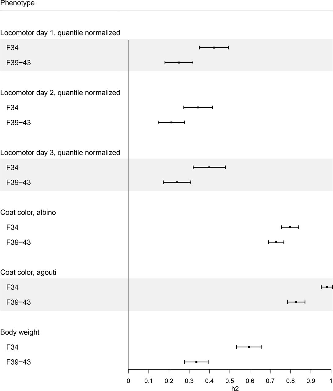
All heritability estimates are highly significant (p < 1.0×10-05; see S7 Table).
Due to the high genetic correlations (S6 Table), we suspected that a mega-analysis using the combined sample set would allow for the identification of additional loci; indeed, mega-analysis identified four novel genom×10-wide significant associations (Fig 4; S9 Table). The significance of the associations identified by the mega-analysis was often greater than in either individual cohort. For instance, the p-values obtained by mega-analysis for chr4:66866758 (p = 1.64×10⁻⁹) and chr14:82672838 (p = 2.06×10⁻¹⁰) for body weight were lower than the corresponding p-values for the same loci for F34 (chr4:65246120, p = 9.06×10⁻⁸; chr14:78926547, p = 6.24×10⁻⁶) and F39-43 (chr4:66414508, p = 8.06×10⁻⁸; chr14:79312393, p = 7.53×10⁻⁶; S7 Fig).

Mega-analysis identified a locus on chromosome 10 (chr10.104988207) that was not detected in the F34 or F39-F43 alone, suggesting that mega-analysis enhanced power to detect some loci.
Discussion
We used F34 and F39-43 generations of a LG/J × SM/J AIL to perform GWAS, SNP heritability estimates, genetic correlations, replication and mega-analysis. We had previously performed several GWAS using a sparse marker set in the F34 cohort. In this study we used a denser set of SNPs, obtained using GBS, to reanalyze the F34 cohort. We found 110 significant loci, 36 of which had not been identified in our prior studies using the sparse marker set. We used a new, previously unpublished F39-43 cohort to show that some by not all loci replicated across cohorts. We also found that genetic correlations were high from most traits measured in both cohorts. Imputation to reference panels increased the number of SNPs available for analysis but did not meaningfully enhance the number of loci we discovered because it did not improve our ability to capture recombination events. Taken together, we have identified refined regions of associations for numerous physiological and behavioral traits in multiple generations of AILs, providing resources for future functional validation studies as well as GWAS replication studies.
Previous publications from our lab used a sparse set of array genotypes for GWAS of various behavioral and physiological traits in 688 F34 AILs (16,17,35–38,40,41). In this study we obtained a much denser marker set for 428 of the initial 688 AIL mice using GBS. The denser genotypes allowed us to identify most of the loci obtained using the sparse set, as well as many additional loci. For instance, using the sparse markers we identified significant locus on chromosome 8 for locomotor day 2 activity that contained only one gene: Csmd1 (CUB and sushi multiple domains 1). Gonzales et al. (39) replicated this finding in F50-56 AIL and identified a cis-eQTL mapped to the same region. Csmd1 mutant mice showed increased locomotor activity compared to wild-type and heterozygous mice, indicating that Csmd1 is likely a causal gene for locomotor and related traits (39). We replicated this locus in the r×10-analysis of the F34 cohort that used the denser marker set (S7 Fig). We also replicated a locus on chromosome 17 for distance traveled in the periphery in the open field test (Fig 4; (36,39)), three loci on chromosomes 4, 6, and 14 for body weight (Supplementary Fig 7; (40)), one locus on chromosome 7 for mean corpuscular hemoglobin concentrations (MCHC, complete blood count; S7 Fig; (41)), and numerous loci on chromosome 4, 6, 7, 8, and 11 for muscle weights (Supplementary Fig 7; (37)). We noticed that even using original spares markers, some previously published loci were not replicated in the current GWAS. The most likely explanation is that we had only 428 of the 688 mice used in the previous publications. Methodological differences between prior studies and the current study, such as the use of QTLRel rather than GEMMA and the choice of pedigree rather than genotypes for estimating relatedness, may also lead to lack of complete replication [56].
F39-43 AILs replicated some, but not all, significant loci identified in F34, despite generally high genetic correlations between the two cohorts. Significant loci for coat color, which are monogenic and served as positive controls, were consistent between the two cohorts. Loci for body weight were fully replicated (p<0.05) between F34 and F39-43, while loci for locomotor activity were not. Nevertheless, the beta estimates for all but two loci shared the same sign, which provides modest evidence for replication. Several possibilities may cause the lack of replication for locomotor activity. Firstly, unlike the F34 dataset, the F39-43 used multiple technicians to conduct the behavioral tests and occurred over a prolonged period of time in which numerous environmental factors may have changed. The circumstances under which the F39-43 data were collected may have introduced greater environmental differences, possibly contributing to their lower heritability and the limited replication. Secondly, the loci for locomotor activity identified in F34 could be false positives. However, given that our F34 results replicated the same locus on chromosome 8 as in F50-56 (39), we believe that these loci are true discoveries. Future studies in other AIL cohorts should attempt to replicate the loci for locomotor activity again.
We performed a mega-analysis using F34 and F39-43 AIL mice. The combined dataset increased our power and allowed us to identify four novel genome-wide significant associations that were not detected in either the F34 or the F39-43 cohorts. For example, the mega-analysis identified a locus for body weight on chromosome 2 (Fig S7). Parker et al. (40) identified the same locus using an integrated analysis of LG/J × SM/J F2 and F34 AILs.
LD in the LG/J × SM/J AIL mice is more extensive than in the Diversity Outbred mice and Carworth Farms White mice (1). Some of the loci that we identified are relatively large, making it difficult to infer which genes are responsible for the association. We focused on loci that contained 5 or fewer genes (Table 1). We highlight a few genes that are supported by the existing literature for their role in the corresponding traits. The lead SNP at chr1:77255381 is associated with tibia length in F34 AILs (Table 1; S7 Fig). One gene at this locus, EphA4, codes for a receptor for membrane-bound ephrins. EphA4 plays an important role in the activation of the tyrosine kinase Jak2 and the signal transducer and transcriptional activator Stat5B in muscle, promoting the synthesis of insulin-like growth factor 1 (IGF-1) (64–66). Mice with mutated EphA4 shows significant defect in body growth (66). Curiously, another gene at this locus, Pax3, has been shown as a transcription factor expressed in resident muscle progenitor cells and is essential for the formation of skeletal muscle in mice (67). It is possible that both EphA4 and Pax3 are associated with the trait tibia length because they are both involved in organismal growth. Another region of interest is the locus at chr4:66866758, which is associated with body weight in all AIL cohorts (Table 1; S4 Table; S8 Table; S9 Table). The lead SNP is immediately upstream of Tlr4, Toll-like receptor 4, which recognizes Gram-negative bacteria by its cell wall component, lipopolysaccharide (68,69). TLR4 responds to the high circulating level of fatty acids and induces inflammatory signaling, which leads to insulin resistance (70). Kim et al showed TLR4-deficient mice were protected from the increase in proinflammatory cytokine level and gained less weight than wild-type mice when fed on high fat diet (71). The association between Tlr4 and body weight in the AILs corroborates these findings.
Many GWAS use a 1.0~2.0 LOD support interval to approximate the size of the association region (see (72,73)). The LOD support interval, proposed by Conneally et al. (74) and Lander & Botstein (75), is a simple confidence interval method involving converting the p-value of the peak locus into a LOD score, subtracting “drop size” from the peak locus LOD score, and finding the two physical positions to the left and to the right of the peak locus location that correspond to the subtracted LOD score. Although Mangin et al. (76) showed via simulation that the boundaries of LOD support intervals depend on effect size, others observed that a 1.0 ~ 2.0 LOD support interval accurately captures ~95% coverage of the true location of the loci when using a dense set of markers (75,77,78). In the present study, we considered using LOD support intervals but found that the sparse array SNPs produced misleadingly large support intervals. Various methods have been proposed for calculating confidence intervals in analogous situations (e.g. (12,79)). Rather than adopting a formal method, we performed credible set analysis and compared LocusZoom plots of the same locus region between array SNPs and the GBS SNPs (S7 Fig; (80)). For example, the benefit of the denser SNP coverage is easily observed in the locus on chromosome 7 (array lead SNP chr7:44560350; GBS lead SNP chr7:44630890) for the complete blood count trait “retic parameters cell hemoglobin concentration mean, repeat” (Fig S7). Thus, there are advantages of dense SNP sets that go beyond the ability to discover additional loci.
Our study has notable limitations. First, not all F34 and F39-43 animals that were phenotyped were later genotyped by GBS due to missing DNA samples, which in turn lowered our sample size and reduced the power of association analyses. Second, F39-43 traits have been collected by different technicians over the span of several years, which introduced noise and diminished trait heritability (Fig 2).
The present study explored the role of marker density and imputation in GWAS. Furthermore, the combination of denser marker coverage and the addition of 600 F39-43 AIL mice allowed us to identify novel loci for locomotor activity, open field test, fear conditioning, light dark test for anxiety, complete blood count, iron content in liver and spleen, and muscle weight. Our findings add to the large body of phenotypic/genotypic data available for the LG/SM AIL, which can be found on GeneNetwork [http://www.genenetwork.org].
Materials and Methods
Animals
All mice used in this study were members of the advanced intercross line (AIL) between LG/J and SM/J that was originally created by Dr. James Cheverud (Loyola University Chicago, Chicago, IL). The AIL line has been maintained in the Palmer laboratory since generation F33. Age and exact number of animals tested in each phenotype are described in S1 Table. Several previous publications (16,35–38,40,41) have reported on association analyses of the F34 mice (n=428). No prior publications have described the F39-43 generations (n=600). The sample size of F34 mice reported in this study (n=428) is smaller than that in previous publications of F34 (n=688) because we only sequenced a subset of F34 animals using GBS. With the exception of coat color and locomotor activities, we quantile normalized all phenotypes. Coat color traits were coded in binary numbers (albino: 1 = white, 0 = non-white; agouti: 1 = tan, 0 = black, NA=white). Locomotor activity traits were not quantile transformed in order to follow the guideline described in Cheng et al. (35) for direct comparison.
F34, F39-43 Phenotypes
We have previously described the phenotyping of F34 animals for locomotor activity (35), fear conditioning (36), open field (36), coat color, body weight (40), complete blood counts (41), heart and tibia measurements (37), muscle weight (37). Iron content in liver and spleen, which have not been previously reported in these mice, was measured by atomic absorption spectrophotometry, as described in Gardenghi et al. (81) and Graziano, Grady and Cerami (82). Although the phenotyping of F39-43 animals has not been previously reported, we used method that were identical to those previously reported for locomotor activity (35), open field (36), coat color, body weight (40), and light/dark test for anxiety (15).
F34 AIL Array Genotypes
F34 animals had been genotyped on a custom SNP array on the Illumina Infinium platform (35,36), which yielded a set of 4,593 SNPs on autosomes and X chromosome that we refer to as ‘array SNPs’.
F34 and F39-43 GBS Genotypes
F34 and F39-43 animals were genotyped using genotyping-by-sequencing (GBS), which is a reduced-representation genome sequencing method (1,39). We used the same protocol for GBS library preparation that was described in Gonzales et al (39). We called GBS genotype probabilities using ANGSD (83). GBS identified 1,667,920 autosomal and 43,015 X-chromosome SNPs. To fill in missing genotypes at SNPs where some but not all mice had calls, we ran within-sample imputation using Beagle v4.1, which generated hard call genotypes as well as genotype probabilities (60). After imputation, only SNPs that had dosage r2 > 0.9 were retained. We removed SNPs with minor allele frequency < 0.1 and SNPs with p < 1.0×10⁻⁶ in the Chi-square test of Hardy–Weinberg Equilibrium (HWE) (S2 Table). All phenotype and GBS genotype data are deposited in GeneNetwork (http://www.genenetwork.org).
QC of individuals
We have found that large genetic studies are often hampered by cross-contamination between samples and sample mix-ups. We used four features of the data to identify problematic samples: heterozygosity distribution, proportion of reads aligned to sex chromosomes, pedigree/kinship, and coat color. We first examined heterozygosity across autosomes and removed animals where the proportion of heterozygosity that was more than 3 standard deviations from the mean (S1 Fig). Next, we sought to identify animals in which the recorded sex did not agree with the sequencing data. We compared the ratio of reads mapped to the X and Y chromosomes. The 95% CI for this ratio was 196.84 to 214.3 in females and 2.13 to 2.18 in males. Twenty-two F34 and F39-43 animals were removed because their sex (as determined by reads ratio) did not agree with their recorded sex; we assumed this discrepancy was due to sample mix-ups. To further identify mislabeled samples, we calculated kinship coefficients based on the full AIL pedigree using QTLRel. We then calculated a genetic relatedness matrix (GRM) using IBDLD, which estimates identity by descent using genotype data. The comparison between pedigree kinship relatedness and genetic kinship relatedness identified 7 pairs of animals that showed obvious disagreement between kinship coefficients and the GRM. Lastly, we excluded 14 F39-43 animals that showed discordance between their recorded coat color and their genotypes at markers flanking Tyr, which causes albinism in mice. The numbers of animals filtered at each step are listed in S2 Table. Some animals were detected by more than one QC step, substantiating our belief that these samples were erroneous.
At the end of SNP and sample filtering, we had 59,561 autosomal and 831 X chromosome SNPs in F34, 58,966 autosomal and 824 X chromosome SNPs in F39-43, and 57,635 autosomal and 826 X chromosome SNPs in the combined F34 and F39-43 set (S2 Table). GBS genotype quality was estimated by examining concordance between the 66 SNPs that were present in both the array and GBS genotyping results.
LD decay
Average LD (r2) was calculated using allele frequency matched SNPs (MAF difference < 0.05) within 100,000bp distance, as described in Parker et al. (1).
Imputation to LG/J and SM/J reference panels
F34 array genotypes (n=428) and F34 GBS genotypes (n=428) were imputed to LG/J and SM/J whole genome sequence data (59) using BEAGLE. For F34 array imputation, we used a large window size (100,000 SNPs and 45,000 SNPs overlap). Imputation to reference panels yielded 4.3 million SNPs for F34 array and F34 GBS imputed sets. Imputed SNPs with DR2 > 0.9, MAF > 0.1, HWE p value > 1.0×10⁻⁶ were retained, resulting in 4.1M imputed F34 GBS SNPs and 4.3M imputed F34 array SNPs.
Genome-wide association analysis (GWAS)
We used the linear mixed model, as implemented in GEMMA (52), to perform a GWAS that accounted for the complex familial relationships among the AIL mice (35,39). We used the leave-one-chromosome-out (LOCO) approach to calculate genetic relatedness matrix, which effectively circumvented the problem of proximal contamination (54). Separate GWAS were performed using F34 array genotypes, F34 GBS genotypes, and F39-43 GBS genotypes. Apart from coat color (binary trait) and locomotor activity, raw phenotypes were quantile normalized prior to analysis. Locomotor activity was not quantile normalized because the trait was reasonably normally distributed already and because we wanted our analysis to match those performed in Cheng et al (35). Because F34 AIL had already been studied using array genotypes (35) and mapped using QTLRel (63), we used the same covariates as described in Cheng et al. (35) in order to examine whether our array and GBS GWAS would replicate their findings. We included sex and body weight as covariates for locomotor activity traits (see covariates used in (35))and sex, age, and coat color as covariates for fear conditioning and open field test in F34 AILs (see covariates used in (36)). We used sex and age as covariates for all other phenotypes. Covariates for each analysis are shown in S1 Table. Finally, we performed mega-analysis of F34 and F39-43 animals (n=1,028) for body weight, coat color, and locomotor activity, since these traits were measured in the same way in both cohorts. For the mega-analyses, locomotor activity was quantile normalized after the combination of the two datasets to ensure that data were normally distributed across generations.
Identifying suspicious SNPs
Some significant SNPs in F34 GWAS and in the mega-analysis of F34 and F39-43 were suspicious because nearby SNPs, which would have been expected to be in high LD (a very strong assumption in an AIL), did not have high −log10 values. We only examined SNPs that obtained significant p-values; these examinations reveled that these SNPs had suspicious ratios of heterozygotes to homozygotes calls and had corresponding HWE p-values that were close to our 1.0×10⁻⁶ threshold (S10 and S11 Tables). To avoid counting these as novel loci, we removed those SNPs prior to summarizing our results as they likely reflected genotyping errors.
Selecting independent significant SNPs
To identify independent “lead loci” among significant GWAS SNPs that surpass the significance threshold, we used the LD-based clumping method in PLINK v1.9. We empirically chose clumping parameters (r2 = 0.1 and sliding window size = 12,150kb) that gave us a conservative set of independent SNPs (S3 Table). For the coat color phenotypes, we found that multiple SNPs remained significant even after LD-based clumping, presumably due to the extremely significant associations at these Mendelian loci. In these cases, we used a stepwise model selection procedure in GCTA (62) and performed association analyses conditioning on the most significant SNPs.
Significance thresholds
We used MultiTrans and SLIDE to set significance thresholds for the GWAS (56,57). MultiTrans and SLIDE are methods that assume multivariate normal distribution of the phenotypes, which in LMM models, contain a covariance structure due to various degrees of relatedness among individuals. We were curious to see whether MultiTrans/SLIDE produces significance thresholds drastically different from the threshold we obtained from a standard permutation test (‘naïve permutation’ as per Cheng et al. (54)). We performed 1,000 permutations using the F34 GBS genotypes and the phenotypic data from locomotor activity (days 1, 2, and 3). We found that the 95th percentile values for these permutations were 4.65, 4.79, and 4.85, respectively, which were very similar to 4.85, the threshold obtained from MultiTrans using the same data. Thus, the thresholds presented here were obtained from MultiTrans but are similar (if anything slightly more conservative) than thresholds we would have obtained had we used permutation. Because the effective number of tests depends on the number of SNPs and the specific animals used in GWAS, we obtained a unique adjusted significance threshold for each SNP set in each animal cohort (S12 Table).
Credible set analysis
We followed the method described in (50). The R script could be found on GitHub: https://github.com/hailianghuang/FM-summary/blob/master/getCredible.r
Genetic correlation and heritability estimates between F34 and F39-43 phenotypes
Locomotor activity, body weight, and coat color had been measured in both F34 and F39-43 populations. We calculated both SNP heritability and genetic correlations between F34 and F39-43 animals using GCTA bivariate GREML analysis (62). Because F39-43 day 1 locomotor activity data were not normally distributed, we quantile normalized locomotor activity data when estimating SNP heritabilities and genetic correlations.
LocusZoom Plots
LocusZoom plots were generated using the standalone implementation of LocusZoom (80), using LD scores calculated from PLINK v.1.9 --ld option and mm10 gene annotation file downloaded from USCS genome browser.
Ethics Statement
All procedures were approved by the Institutional Animal Care and Use Committee (IACUC protocol: S15226) Euthanasia was accomplished using CO2 asphyxiation followed by cervical dislocation.
Supporting information
S1 Fig. Autosomal heterozygosity distribution in F34, F39-43 AILs. Animals with excessive or insufficient heterozygosity (3 s.d. away from mean) were removed from further analysis. As controls, we have sequenced two F2s of LG and SM, four LG mice and four SM mice (see annotated data points with 1 and 0 heterozygosity).
S2 Fig. Kinship coefficients in F34 and F39-43 AILs calculated from pedigree against genetic relatedness matrix calculated using IBDLD [49]. Each circle represents a pair of animals, which their genetic kinship relatedness on the x-axis and pedigree kinship relatedness on the y-axis. Color signifies relatedness based on AIIL pedigree. Blue circles represent identical twins, red full siblings, yellow parent-offspring pairs, grey other relationships. Seven animal pairs that deviate from the pedigree relationship clusters were excluded (see black arrows).
S3 Fig. Heatmap showing F34 array and F34 GBS genotype concordance in percentages, using 66 shared SNPs. “A” codes for the LG/J allele, and “B” codes for the SM/J allele. “AA” genotype concordance between array and GBS is 24.54%, “AB” 43.23%, “BB” 27.60%.
S4 Fig. LD decay in F34 array, F34 GBS, F39-43 GBS, and F34 and F39-43 GBS SNP sets.
S5 Fig. Manhattan plots comparing 4,593 F34 array, 60.3K F34 GBS, 4.3M imputed F34 array, and 4.1M imputed F34 GBS (N=428) SNPs on day 2 locomotor activity. Adjusted significance thresholds for imputed array and GBS SNPs were estimated using LD pruned SNPs (r2=0.1, window size=20kb; PLINK v1.9). Notice that even though the imputed sets have more SNPs (the two right panels), they are frequently blocks of many SNPs with almost identical position and LD=1, therefore making it hard to visualize the additional SNPs.
S6 Fig. SNP heritability using F34 GBS and F34 array SNPs (slope=1).
S7 Fig. LocusZoom for F34 array, F34 GBS, F39-43 GBS, and mega-analysis QTLs. Purple track shows the credible set interval (r2 threshold = 0.8, posterior probability threshold = 0.99).
S1 Table. List of phenotypes used in GWAS.
S2 Table. SNP and individual QC filter table. Numbers of animals and SNPs remained after each step of filtering are shown per GBS SNP set.
S3 Table. Effect of PLINK v1.9 clump-based pruning parameters on number of independent SNPs remained. At all r2 values examined, a sliding window size of 12150kb was the first smallest window that yield the most stringent number of clumped SNPs in both array and GBS GWAS.
S4 Table. Lead QTL in F34 GBS and F34 array GWAS studies across phenotypes. Significant SNPs are clumped using parameters r2=0.1, 12150kb.
S5 Table. F34 GBS and array SNP heritability estimates.
S6 Table. F34 and F39-43 genetic correlations in locomotor activity, coat color, and body weight.
S7 Table. SNP-heritability comparison between F34 and F39-43 GBS.
S8 Table. Lead QTL in F39-43 N=600 GBS GWAS studies across phenotypes. Significant SNPs are clumped using parameters r2=0.1, 12150kb.
S9 Table. Lead QTL in F34 and F39-43 (N=1028) mega-analysis across phenotypes. Significant SNPs are clumped using parameters r2=0.1, 12150kb.
S10 Table. SNPs in F34 GBS set with HWE p-values close to 1.0×10⁻⁶ cutoff threshold. These SNPs are removed from QTL summary tables.
S11 Table. SNPs in F34 and F39-43 mega-analysis GBS set with HWE p values close to 1.0×10⁻⁶ cutoff threshold. These SNPs are removed from QTL summary tables.
S12 Table. Adjusted significance threshold for each SNP set and GWAS cohort.
Acknowledgements
We would like to recognize Jackie Lim and Kaitlin Samocha for collecting F34 AIL phenotype data and Ryan Walters for collecting F39-43 AIL phenotype data. We wish to acknowledge Alex Gileta for input on a draft of this manuscript.
Footnotes
Data Availability All relevant data are within the paper and its Supporting Information files. Genotypes and phenotypes of F34 (“AIL LGSM F34 (Array)”: GN655; “AIL LGSM F34 (GBS)”: GN656), F39-43 (“AIL LGSM F39-43 (GBS)”: GN657), and mega-analysis cohort (“AIL LGSM F34 and F39-43 (GBS)”: GN654) of AIL are uploaded to GeneNetwork2 (http://gn2.genenetwork.org/).
Author contributions XZ imputed genotypes, performed SNP and individual QC, and conducted GWAS in F34 and F39-43 AILs under supervision of AAP. AAP also provided computational resources for the analyses in this paper. CS prepared GBS libraries for sequencing, as well as organizing portions of the F39-43 phenotypes. NMG de-multiplexed GBS sequencing results and performed alignment and variant calling. RC helped with kinship relatedness matrix calculated from AIL pedigree. AC provided technical support for running programs and scripts. GS collected F39-43 phenotypes, respectively. XZ co-wrote the manuscript with AAP, who designed the study and oversaw data collection.
References
- 1.↵
- 2.
- 3.
- 4.
- 5.
- 6.
- 7.
- 8.
- 9.
- 10.
- 11.
- 12.↵
- 13.
- 14.
- 15.↵
- 16.↵
- 17.↵
- 18.↵
- 19.↵
- 20.↵
- 21.↵
- 22.↵
- 23.↵
- 24.
- 25.
- 26.
- 27.↵
- 28.↵
- 29.↵
- 30.
- 31.↵
- 32.↵
- 33.↵
- 34.↵
- 35.↵
- 36.↵
- 37.↵
- 38.↵
- 39.↵
- 40.↵
- 41.↵
- 42.↵
- 43.
- 44.↵
- 45.↵
- 46.
- 47.↵
- 48.↵
- 49.↵
- 50.↵
- 51.↵
- 52.↵
- 53.↵
- 54.↵
- 55.↵
- 56.↵
- 57.↵
- 58.↵
- 59.↵
- 60.↵
- 61.↵
- 62.↵
- 63.↵
- 64.↵
- 65.
- 66.↵
- 67.↵
- 68.↵
- 69.↵
- 70.↵
- 71.↵
- 72.↵
- 73.↵
- 74.↵
- 75.↵
- 76.↵
- 77.↵
- 78.↵
- 79.↵
- 80.↵
- 81.↵
- 82.↵
- 83.↵


