

Abstract
Mutation and recombination are key evolutionary processes governing phenotypic variation and reproductive isolation. We here demonstrate that biodiversity within all globally known strains of Schizosaccharomyces pombe arose through admixture between two ancestral lineages. Initial hybridization occurred ∼20 sexual outcrossing generations ago consistent with recent, human-induced migration at the onset of intensified transcontinental trade. Species-wide phenotypic variation was explained near-exclusively by strain-specific arrangements of alternating ancestry components with evidence for transgressive segregation. Reproductive compatibility between strains was likewise predicted by the degree of shared ancestry. Over 800 structural mutations segregating at low frequency had overall little effect on the introgression landscape. This study sheds new light on the population history of S. pombe and illustrates the importance of hybridization as a creative force in generating biodiversity.
Introduction
Mutation is the ultimate source of biodiversity. In sexually reproducing organisms it is assisted by recombination shuffling mutations of independent genomic backgrounds into millions of novel combinations. This widens the phenotypic space upon which selection can act and thereby accelerates evolutionary change (Muller, 1932; Fisher, 1999; McDonald et al., 2016). This effect is enhanced for heterospecific recombination between genomes of divergent populations (Abbott et al., 2013). Novel combinations of independently accumulated mutations can significantly increase the overall genetic and phenotypic variation, even beyond the phenotypic space of parental lineages (transgressive segregation (Lamichhaney et al., 2017; Nolte and Sheets, 2005)). Yet, if mutations of the parental genomes are not compatible to produce viable and fertile offspring, hybridization is a dead end. Phenotypic variation then remains within the confines of genetic variation of each reproductively isolated, parental lineage.
It is increasingly recognised that hybridisation is commonplace in nature, and constitutes an important driver of diversification (Abbott et al., 2013; Mallet, 2005). Ancestry components of hybrid genomes can reach from clear dominance of the more abundant species (Dowling et al., 1989; Taylor and Hebert, 1993), over a range of admixture proportions (Lamichhaney et al., 2017; Runemark et al., 2018) to the transfer of single adaptive loci (The Heliconius Genome Consortium et al., 2012). The final genomic composition is determined by a complex interplay of demographic processes, heterogeneity in recombination (e.g. induced by genomic rearrangements) (Wellenreuther and Bernatchez, 2018) and selection (Sankararaman et al., 2014; Schumer et al., 2016). Spurred by rapid progress in sequencing technology, genome-wide assays now allow characterizing patterns of admixture and illuminate the underlying processes (Payseur and Rieseberg, 2016). Yet, research has largely focused on animals (Jay et al., 2018; Meier et al., 2017; Turner and Harr, 2014; Vijay et al., 2016) and plants (Twyford et al., 2015) characterized by large genomes and long generation times. Surprisingly little attention has been paid to natural populations of sexually reproducing micro-organisms (Leducq et al., 2016; Stukenbrock, 2016; Steenkamp et al., 2018). The fission yeast Schizosaccharomyes pombe is an archiascomycete haploid unicellular fungus with a facultative sexual mode of reproduction. Despite of its outstanding importance as a model system in cellular biology (Hoffman et al., 2015) and the existence of global sample collections, essentially all research has been limited to a single isogenic strain isolated by Leupold in 1949 (Leupold 972; JB22 in this study). Very little is known about the ecology, origin, and evolutionary history of the species (Jeffares, 2018). Global population structure is shallow with no apparent geographic stratification (Jeffares et al., 2015). Genetic diversity (π = 3×10⁻³ substitutions/site) appears to be strongly influenced by genome-wide purifying selection with the possible exception of region-specific balancing selection (Fawcett et al., 2014; Jeffares et al., 2015). Despite the overall low genetic diversity S. pombe shows abundant additive genetic variation in a variety of phenotypic traits including growth, stress responses, cell morphology, and cellular biochemistry (Jeffares et al., 2015). The remarkable worldwide lack of genetic structure is not only at odds with large phenotypic variation between strains but likewise contrasts with evidence for post-zygotic reproductive isolation between inter-strain crosses ranging from 1% to 90 % of spore viability (Jeffares et al., 2015; Kondrat’eva and Naumov, 2001; Teresa Avelar et al., 2013; Zanders et al., 2014; Naumov et al., 2015; Marsellach, 2017).
In this study, we integrate whole-genome sequencing data from three different technologies - sequencing-by-synthesis (Illumina technology), single-molecule real-time sequencing (Pacific BioSciences technology) and nanopore sequencing (Oxford Nanopore technology) - sourced from a mostly human-associated, global sample collection to elucidate the evolutionary history of the S. pombe complex. Using population genetic analyses based on single nucleotide polymorphism (SNP) we show that global genetic variation of S. pombe results from recent hybridization of two ancient lineages. 25 de novo assemblies from 17 divergent strains further allowed us to quantify segregating structural variation including insertions, deletions, inversion and translocations. In light of these findings, we retrace the global population history of the species, and discuss the relative importance of genome-wide ancestry and structural mutations in explaining the large variation in phenotype and reproductive isolation.
Results
Global genetic variation in S. pombe is characterized by ancient admixture
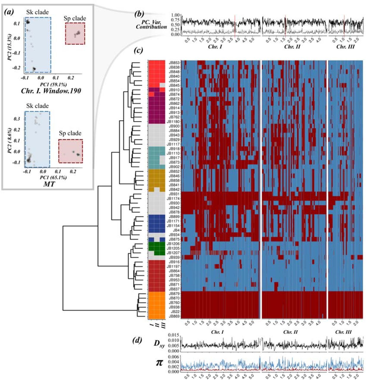
Genetic variation of the global S. pombe collection comprises 172,935 SNPs segregating in 161 individuals. It can be sub-structured into 57 clades that differ by more than 1900 variants, but are near-clonal within (Jeffares et al., 2015). We divided the genome into 1925 overlapping windows containing 200 SNP each. Principle component analysis conducted on orthologous windows for one representative of each clade showed a highly consistent pattern along the genome (Figure 1a, Supplementary Figure 1): the major axis of variation (PC1) split all samples into two discrete groups explaining 60% ± 13% of genetic variance (Figure 1b). All samples fell into either extreme of the normalized distribution of PC1 scores (PC1 ∈ [0; 0.3] ∪ [0.7; 1]) (Supplementary Figures 2 and 3) with the only exception of strains with inferred change in ploidy (Methods, Supplementary Figure 4). PC2 explained 13% ± 6% of variation and consistently attributed higher variation to one of the two groups.

(a) Example of principal component analysis (PCA) of a representative genomic window in chromosome I (top) and the whole mitochondrial DNA (bottom). Samples fall into two major clades, Sp (red square) and Sk (blue square). The proportion of variance explained by PC1 and PC2 is indicated on the axis labels. Additional examples are found in Supplementary Figure 1 (b) Proportion of variance explained by PC1 (black line) and PC2 (grey line) for each genomic window along the genome. Centromeres are indicated with red bars. Note the drop in proximity to centromeres and telomeres where genotype quality is significantly reduced. (c) Heatmap for one representative of 57 near-clonal groups indicating ancestry along the genome (right panel). Samples are organised according to a hierarchical clustering, grouping samples based on ancestral block distribution (left dendrogram). Colours on the tips of the cladogram represent cluster membership by chromosome (see Supplementary Figure 7). Samples changing clustering group between chromosomes are shown in grey. (d) Estimate of Dxy between ancestral groups and genetic diversity (π) within the Sp and Sk clade along the genome.

(a) Proportion of Sp (red) and Sk (blue) ancestry across all 57 samples along the genome. (b) Tajima’s D differentiated by Sp (red) and Sk (blue) ancestry and pooled across all samples irrespective of ancestry (grey line). Genomic regions previously identified under purifying selection (Fawcett et al., 2014) are shown with black triangles. Reported active meiotic drives (Zanders et al., 2014; Hu et al., 2017; Nuckolls et al., 2017) are indicated by yellow triangles. The third panel shows the difference between ancestry specific Tajima’s D and the estimate for the pooled samples.
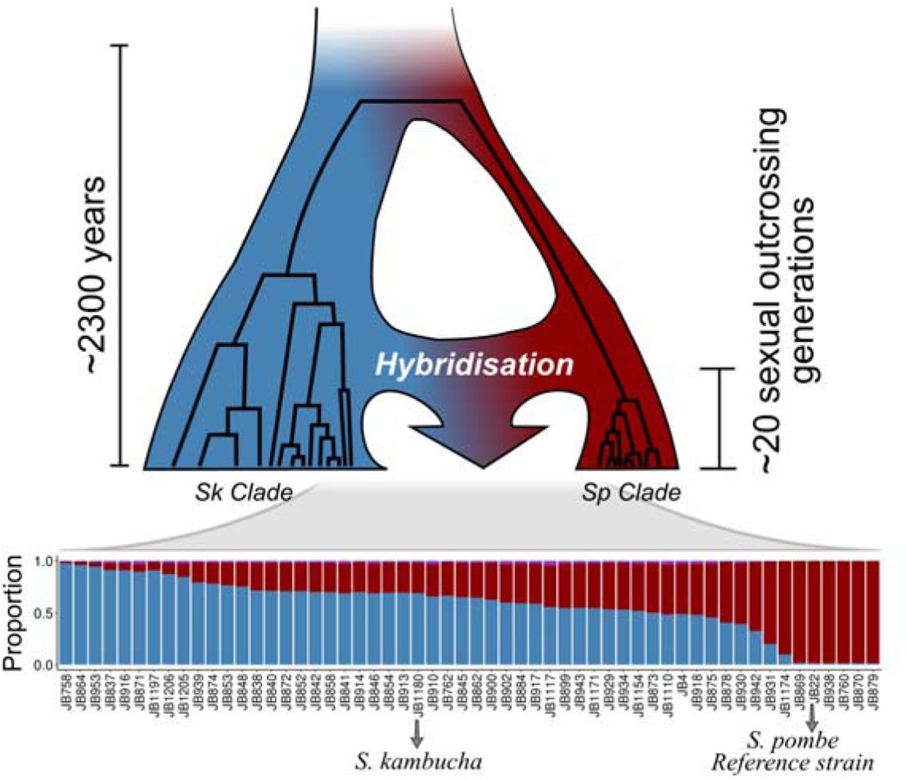
An ancestral population diverged into two major clades, Sp (red) and Sk (blue) approximately 2300 years ago (Jeffares et al., 2015). Recurrent hybridization upon secondary contact initiated around 20 sexual outcrossing generations ago resulted in admixed genomes with a range of admixture proportions (bottom) prevailing today.

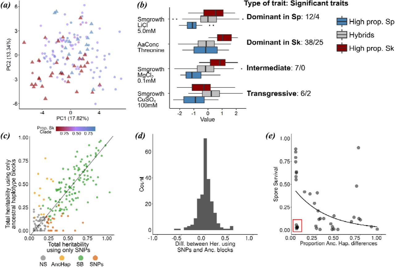
(a) PCA of normalized phenotypic variation across 228 traits. The proportion of variance explained by PC1 and PC2 is indicated on the axis labels. Admixed samples are coloured coded by ancestry proportion (cf. Figure 3) ranging from pure Sp (red triangle) to pure Sk (blue triangle) ancestry. (b) Phenotypic distribution of example traits separated by the degree of admixture: admixed samples are shown in grey, pure ancestral Sp and Sk samples are shown in red and blue, respectively. The number of traits corresponding to a dominant, additive and transgressive genetic architecture is indicated on the right hand side (before/after multiple testing correction) (c) Comparison of heritability estimates of all 228 traits based on 172,935 SNPs (abscissa) and on 1925 genomic windows polarized by ancestry (ordinate). Colours indicate statistical significance. NS: heritability values not significantly different from zero, AncHap: significant only using ancestral blocks, SNPs: significant only using SNPs, SB: significant in both analyses. Diagonal (slope=1) added as reference. (d) Histogram of the difference between heritability estimates using SNPs and ancestry components for all 228 traits. (e) Correlation between the difference in ancestry proportions between two strains (cf. Figure 2) and spore viability of the cross. Red box shows samples with low spore viability but high genetic similarity.
This strong signal of genomic windows separating into two discrete groups suggested that the genomic diversity in this collection was derived from two distinct populations. Systematic differences between groups were likewise reflected in population genetic summary statistics including Watterson’s theta (θ), pairwise nucleotide diversity (π), and Tajima’s D (Figure 1d and 2b). Significant differences in these statistics (Kendall’s τ p-value ≤ 2.2×10⁻¹⁶), also holding true for mitochondrial genetic variation (Figure 1a), allowed polarising groups across windows into a ‘low-diversity’ group (red) and a ‘high-diversity group (blue) (Figure 1a, Supplementary Figure 5). Genetic divergence between groups (Dxy) was 15 and 3 times higher than mean genetic diversity within each group, respectively, and thus supports a period of independent evolution. Painting genomic windows by group membership revealed blocks of ancestry distributed in sample specific patterns along the genome (Figure 1c, Supplementary Figure 6). Grouping samples by the pattern of genomic ancestry across the genome revealed 8 discrete clusters. These clusters resemble clusters of strains previously obtained by Structure and fineStructure using the whole genome (Jeffares et al., 2015). Consistent with independent segregation of linkage groups, membership differed between chromosomes (Figure 1c) and genome components (Supplementary Figures 7 & 8). The sample corresponding to the reference genome isolated originally from Europe (Leupold’s 972; JB22) consisted almost exclusively of ‘red’ ancestry (>96% red), whereas other samples were characterized near-exclusively by ‘blue’ ancestry (>96% blue). The sample considered to be a different species from Asia, S. kambucha (JB1180 (Singh and Klar, 2002)) had a large proportion of ‘blue’ windows (>70% blue). Hereafter, we refer to the ‘red’ and ‘blue’ clade as Sp and Sk, respectively.

(a) Schematic representation of the three chromosomes in different strains displaying SVs larger than 10kb relative to reference genome JB22 (left panel). Chromosome arms are differentiated by colour; orientation is indicated with arrows relative to the reference; black bars represent centromeres. In the second panel, additional SV, their type and ID of the corresponding strain are illustrated in brackets. (b) Size distribution of SVs below10 kb. Colours indicate the type of SV. (c) Distribution of SV density along the genome. Black bars represent centromeres. (d) Two-dimensional, folded site frequency spectrum between inferred ancestral populations for all SVs, SNPs and LTR INDELs. Numbers and colours show the percentage of the total number of variants in each category. Variants with low frequency in both populations are shown in the blue box. Variants highly differentiated between populations are show in red boxes with total in the upper right box. Fills with percentage lower than 0.01 are empty.
The distribution of ancestry components was highly heterogeneous across the chromosome (Figure 2a, Supplementary Figure 6). Most strains showed an excess of Sp ancestry in parts of chromosome 1, whereas several regions of chromosome 3 had an access of Sk ancestry. Failing to incorporate genome-wide variation of admixture proportions can mimic signatures of selection. For example, equal ancestry contributions yield high positive values of both Tajima’s D (Supplementary Figure 9) and π and may be mistaken as evidence for balancing selection. Strong skew in ancestry proportions reduces both statistics to values of the prevailing ancestry and may appear as evidence for selective sweeps (Figure 2b). Taking ancestry into account, however, there was no clear signature of selection in either Sp or Sk genetic variation that could account for heterogeneity in the genetic composition of hybrids (Supplementary Figure 9). Signatures of selection identified previously (cf. Fawcett et al., 2014) thus likely reflect skewed ancestry proportions rather than events of positive or balancing selection in the ancestral populations.
Overall, these results provide evidence for the presence of at least two divergent ancestral populations: one genetically diverse group (Sk clade) and a less diverse group (Sp clade). The range of admixture proportions and the variety of ancestry patterns along the genome falling into 8 major groups are suggestive of recurring admixture upon secondary contact.
Age of ancestral lineages and timing of hybridisation
Next, we estimated the age of the parental lineages and the time of initial hybridization. Calibrating mitochondrial divergence by known collection dates over the last 100 years, Jeffares et al. (2015) estimated that the time to the most recent common ancestor for all samples dates back to around 2,300 years ago. Current overrepresentation of near-pure Sp and Sk in Europe or Africa / Asia, respectively, is thus consistent with an independent history of the parental lineages on different continents for the most part of the last millennia (Supplementary Figure 8). Yet, the variety of admixed genomes bears testimony to the fact that isolation has been disrupted by heterospecific gene flow. Using a theoretical model assuming secondary contact with subsequent hybridization (Janzen et al., 2018) we estimated that hybridization occurred within the last 20 sexual outcrossing generations (Figure 3, Supplementary Figures 10 and 11). Considering intermittent generations of asexual reproduction, high rates of haploid selfing and dormancy of spores (Jeffares, 2018) it is difficult to obtain a reliable estimate of time in years. A recent estimate is, however, consistent with hybridization induced by the onset of regular trans-continental human trade between Europe with Africa and Asia (∼14th century) and with the Americas (∼15th century). This fits with the observation that all current samples from the Americas were hybrids, while samples with the purest ancestry stem from Europe, Africa and Asia. Moreover, negative genome-wide Tajima’s D estimates for both ancestral clades (mean ± SD: Sp: −0.8 ± 0.9 Sk: −0.7 ± 0.6) signal a period of recent expansion. This is in concordance with previous work indicating population size increase driven by human migration (Jeffares et al., 2015).
Phenotypic variation and reproductive isolation are governed by ancestry components
Next, we assessed the consequences of hybridisation on phenotypic variation making use of a large data set including 228 quantitative traits collected from strains under consideration here (Jeffares et al., 2015). Contrary to genetic clustering of hybrid genomes (Figure 1c), samples with similar ancestry proportions did not group in phenotypic space described by the first two PC-dimensions capturing 31% of the total variance across traits (Figure 4a). Moreover, phenotypic variation of hybrids exceeded variation of pure (>0.9 ancestry) Sp and Sk strains. This was supported by trait specific analyses. We divided samples into three discrete groups: pure Sp, pure Sk and hybrids with a large range of Sp admixture proportions (0.1-0.9). 63 traits showed significant difference among groups, 31 after multiple testing correction (Figure 4b, Supplementary Figures 12). In the vast majority of cases (50 or 29 after multiple testing correction) hybrid phenotypes were indistinguishable from one of the parents, but differed from the other, suggesting dominance of one ancestral background, consistent with some ecological separation of the backgrounds. In 7 cases (0 after multiple testing correction), hybrid phenotypes were intermediate differing from both parents indicative of an additive contribution of both ancestral backgrounds. For several traits (6 or 2 after multiple testing correction) hybrids exceeded phenotypic values of both parents providing evidence for transgressive segregation. Jeffares et al. (2017) showed that the total proportion of variance explained by the additive contribution of genetic variance (used as an estimated of heritability) ranged from 0 to 90%. Across all 228 traits, Sp and Sk ancestry components (Figure 1c) explained an equivalent amount of phenotypic variance as SNPs segregating across all samples, being both highly correlated (Figure 4c, 4d; r = 0.82, p-value ≤ 2.2 · 10-16). This implies that strain-specific combinations of ancestral genetic variation determine overall phenotypic variation with only little contribution from single-nucleotide mutations arising after admixture. In turn, this supports that the formation of hybrids is recent (see above), and little (adaptive) mutations have occurred after it.
Ancestry also explained most of the variation in postzygotic reproductive isolation between strains. Previous work revealed a negative correlation between spore viability and genome-wide SNP divergence between strains (Jeffares et al., 2015). The degree of similarity in genome-wide ancestry had the same effect: the more dissimilar two strains were in their ancestry, the lower the viability of the resulting spores (Figure 4e; Kendall correlation coefficients, τ=259, p-value = 6.66 · 10-3). This finding is consistent with reproductive isolation being governed by many, genome-wide incompatibilities between Sp and Sk. However, in several cases spore survival was strongly reduced in strain combinations with near-identical ancestry. In these cases, reproductive isolation may be caused by few large effect mutations that arose after hybridization.
Structural genetic variation does not determine the distribution of ancestry blocks
Structural genomic changes (structrual variants or SVs hereafter) are prime candidates for large-effect mutations governing phenotypic variation (Jeffares et al., 2017; Küpper et al., 2016), reproductive isolation (Hoffmann and Rieseberg, 2008; Teresa Avelar et al., 2013) and heterospecific recombination (Ortiz-Barrientos et al., 2016). They may thus importantly contribute to shaping heterogeneity in the distribution of ancestry blocks observed along the genome (Jay et al., 2018; Poelstra et al., 2014) (Figure 2b). To test for a possible association of SVs with the skewed ancestry in the genome, we generated chromosome-level de novo genome assemblies for 17 of the most divergent samples using single-molecule real time sequencing (mean sequence coverage 105x; Supplementary Table 7). For the purpose of methodological comparison, we also generated de novo assemblies for a subset of 8 strains (including the reference JB22) based on nanopore sequencing (mean sequence coverage: 140x). SVs were called using a mixed approach combining alignment of de novo genomes and mapping of individual reads to the reference genome JB22. Both approaches and technologies yielded highly comparable results (Methods, Supplementary Figure 13-15 and Supplementary Table 8).
After quality filtering, we retained a total of 832 variant calls including 563 insertions or deletions (indels), 118 inversions, 110 translocations and 41 duplications. The 17 strains we examined with long reads could be classified into six main karyotype arrangements (Figure 5a). The vast majority of SVs were smaller than 10 kb (Figure 5b). The size distribution was dominated by elements of 6 kb and 0.5 kb in length corresponding to known transposable elements (TEs) and their flanking long terminal regions (LTRs), respectively (Kelly and Levin, 2005). Contrary to previous SV classification based on short reads (Jeffares et al., 2017), SV density was not consistently increased in centromeric and telomeric regions (Figure 5c). Only a small number of SVs corresponded to large-scale rearrangements (50 kb - 2.2 Mb) including translocations between chromosomes (Figure 5a). A subset of these have been characterized previously as large-effect modifiers of recombination promoting reproductive isolation (Brown et al., 2011; Teresa Avelar et al., 2013; Jeffares et al., 2017). This includes a 2.1 Mb inversion on chromosome I present in the reference strain(Brown et al., 2011).
Next, we determined the ancestral origin of alleles imputed from SNPs surrounding SV break points. We calculated allele frequencies for SV in both ancestral clades and constructed a folded two-dimensional site frequency spectrum (Figure 5d). The majority of variants (66.3 %) segregated at frequencies below 0.3 in both ancestral genetic backgrounds. Very few SVs were differentiated between ancestral populations (3.2 % of variants with frequency higher than 0.9 in one population and below 0.1 in the other). This pattern contrasted with the reference spectrum derived from SNPs where the proportion of low frequency variants was similar at 59.7 %, but genetic differentiation between populations was substantially higher (20.8 % of SNP variants with frequency higher than 0.9 in one population and below 0.1 in the other). The difference was most pronounced for large SVs (larger than 10 kb) and TEs, where we estimated allele frequencies for all 57 strains by means of PCR and short-read data, respectively. For TE’s, 97.8% of the total 1048 LTR variants segregated at frequencies below 0.3 in both ancestral populations without a single variant differentiating ancestral populations (Figure 5d). Large SVs likewise segregated at low frequencies, being present at most in two strains out of the 57. This included the translocation reported for S. kambucha between chromosome II and III (Zanders et al., 2014), which we found to be specific for that strain. Only the large inversion on chromosome I segregated at higher frequency being present in five strains out of 57, of which three were of pure Sp ancestry including the reference strain (Supplementary Table 10).
In summary, long-read sequencing provided a detailed account of species-wide diversity in structural genetic variation including over 800 high-quality variants ranging from small indels to large-scale inter-chromosomal rearrangements. In contrast to genome-wide SNPs, SVs segregated near-exclusively at low frequencies and were rarely differentiated by ancestral origin. This is consistent with strong diversity-reducing purifying selection relative to SNPs. The fact that SVs, including large-scale rearrangements with known effects on recombination and reproductive isolation (Brown et al., 2011; Teresa Avelar et al., 2013; Zanders et al., 2014), were often unique to single strains precludes a role of SVs in shaping patterns of heterospecific recombination. On the whole, SVs did not determine genome-wide patterns of ancestral admixture, and therefore cannot explain the general observed pattern of reproductive isolation as a function on ancestral similarity (Figure 4e).
Discussion
This study adds to the increasing evidence that hybridization plays an important role as a rapid, ‘creative’ evolutionary force in natural populations (Abbott et al., 2013; Seehausen, 2004; Schumer et al., 2014; Mallet, 2007; Soltis and Soltis, 2009; Abbott et al., 2016; Pennisi, 2016; Nieto Feliner et al., 2017). Heterospecific recombination between two ancestral S. pombe strains shuffled genetic variation of genomes that diverged since classical antiquity about 2,300 years ago. The timing of hybridization coincided with the onset of intensified trans-continental human trade, suggesting an anthropogenic contribution. Admixture is significantly faster than evolutionary change solely driven by mutation. Accordingly, phenotypic variation was near-exclusively explained by ancestry components with only little contribution from novel mutations. Importantly, admixture not only filled the phenotypic space between parental lineages, but also promoted transgressive segregation in several hybrids. This opens the opportunity for hybrids to enter novel ecological niches (Nolte and Sheets, 2005; Pfennig et al., 2016) and track rapid environmental changes (Eroukhmanoff et al., 2013).
Structural mutations are prime candidates for rapid large-effect changes with implications on phenotypic variation, recombination and reproductive isolation (Faria and Navarro, 2010; Ortiz-Barrientos et al., 2016; Wellenreuther and Bernatchez, 2018). This study contributes to this debate providing a detailed account of over 800 high-quality structural variants identified across 17 chromosome level de novo genomes sampled from the most divergent strains within the species. On the whole, SVs had little effect. SVs were kept at low frequencies in both ancestral populations and, contrary to what has been suggested for specific genomic regions in other systems (Jay et al., 2018), they did not account for genome-wide heterogeneity in introgression among strains. They also contributed little to reproductive isolation. While large-scale rearrangements have been shown to affect fitness (Teresa Avelar et al., 2013; Nieuwenhuis et al., 2018) and promote reproductive isolation between specific strains in S. pombe (Brown et al., 2011; Teresa Avelar et al., 2013), reproductive isolation was overall best predicted by the degree of shared ancestry. This suggests a role for negative epistasis between many ancestry-specific loci spread across the genome rather than single major effect mutations such as selfish elements or meiotic drivers (Zanders et al., 2014; Hu et al., 2017; Nuckolls et al., 2017). Additional functional work is needed to identify the genetic elements conveying reproductive isolation.
Material and Methods
Strains
This study is based on a global collection of S. pombe consisting of 161 world-wide distributed strains (see Supplementary Table 1) described in Jeffares et al. (2015).
Inferring ancestry components
To characterize genetic variation across all strains, we made use of publically available data in variant call format (VCF) derived for all strains from Illumina sequencing with an average coverage of around 80x (Jeffares et al., 2015). The VCF file consists of 172,935 SNPs obtained after read mapping to the S. pombe 972 h- reference genome (ASM294v264) (Wood et al., 2003) and quality filtering (see Supplementary Table 1 for additional information). We used a custom script in R 3.4.3 (Team, 2014) with the packages gdsfmt 1.14.1 and SNPRelate 1.12.2 (Zheng et al., 2012, 2017), to divide the VCF file into genomic windows of 200 SNPs with overlap of 100 SNPs. This resulted in 1925 genomic windows of 1 - 89 kb in length (mean 13 kb). For each window, we performed principal component analyses (PCA) using SNPRelate 1.12.2 (Zheng et al., 2012, 2017) (example in Figure 1a and Supplementary Figure 1). The proportion of variance explained by the major axis of variation (PC1) was consistently high and allowed separating strains into two genetic groups/clusters, Sp and Sk (see main text, Figure 1b). We calculated population genetic parameters within clusters including pairwise nucleotide diversity (π) (Nei and Li, 1979), Watterson theta (θw) (Watterson, 1975), and Tajima’s D (Tajima, 1989), as well as the average number of pairwise differences between clusters (Dxy) (Nei and Li, 1979) using custom scripts. Statistical significance of the difference in nucleotide diversity (π) between ancestral clades was inferred using Kendall’s τ as test statistic. Since values of adjacent windows are statistically non-independent due to linkage, we randomly subsampled 200 windows along the genome with replacement. This was repeated a total of 10 times for each test statistic, and we report the maximum p-value. Given the consistent difference between clusters (Figure 1 and Supplementary Figure 2, 3 and 5), normalised PC score could be used to attribute either Sp (low-diversity) or Sk (high-diversity) ancestry to each window (summary statistics for each window are given in Supplementary Table 2). This was performed both for the subset of 57 samples (Figure 1c) and for all 161 samples (Supplementary Figure 6). Using different window sizes (100, 50 and 40 SNPs with overlap of 50, 25 and 20 respectively) yielded qualitatively the same results. Intermediate values in PC1 (between 0.25 and 0.75) were only observed in few, sequential windows where samples transitioned between clusters (Supplementary Figure 3). The only exception was sample JB1207, which we found to be diploid (for details see below).
Population structure after hybridisation
To characterise the genome-wide distribution of ancestry components along the genome, we ran a hierarchical cluster analysis on the matrix containing ancestry information (Sp or Sk) for each window (columns) and strain (rows) using the R package Pvclust 2.0.0 (Suzuki and Shimodaira, 2006). Pvclust includes a multiscale bootstrap resampling approach to calculate approximately unbiased probability values (p-values) for each cluster. We specified 1000 bootstraps using the Ward method and a Euclidian-based dissimilarity matrix. The analysis was run both for the whole genome (Figure 1c) and by chromosome (Figure 1c, Supplementary Figure 7).
Phylogenetic analysis of the mitochondrial genome
From the VCF file, we extracted mitochondrial variants for all 161 samples (Jeffares et al., 2015) and generated an alignment in .fasta format by substituting SNPs into the reference S. pombe 972□h-reference genome (ASM294v264) using the package vcf2fasta (https://github.com/JoseBlanca/vcf2fasta/, version Nov. 2015). A maximum likelihood tree was calculated using RaxML (version 8.2.10-gcc-mpi) (Stamatakis, 2014) with default parameters, GTRGAMMAI approximation, final optimization with GTR□+□GAMMA + I and 1000 bootstraps. The final tree was visualised using FigTree 1.4.3 (http://tree.bio.ed.ac.uk/software/figtree/) (Supplementary Figure 8).
Time of hybridisation
Previous work (Jeffares et al., 2015) has shown that the time to the most recent common ancestor for 161 samples dates back to around 2300 years ago. This defines the maximum boundary for the time of hybridization. We used the theoretical model by Janzen et al., (2018) to infer the age of the initial hybridization event. The model predicts the number of ancestry blocks and junctions present in a hybrid individual as a function of time and effective population size (Ne). First, we obtained an estimate of Ne using the multiple sequential Markovian coalescent (MSMC). We constructed artificial diploid genomes from strains with consistent clustering by ancestry (Figure 1c) and estimated change in Ne as function across time using MSMC 2-2.0.0 (Schiffels and Durbin, 2014). In total we took four samples per group and produced diploid genomes in all possible six pairs for each group, except for one cluster that had only two samples (JB1205 and JB1206). Bootstraps were produced for each analysis, subsampling 25 genomic fragments per chromosome of 200 kb each. Resulting effective population size and time was scaled using reported mutation rate of 2 ñ 10-10 mutations site-1 generation-1 (Farlow et al., 2015). Although it is difficult to be certain of the number of independent hybridization events, it is interesting to see that some clusters show similar demographic histories (Supplementary Figure 16). Regardless of the demographic history in each cluster, long-term Ne as estimated by the harmonic mean ranged between 1 · 105 and 1 · 109. Ne of the near-pure ancestral Sp and Sk cluster was 7 · 105 and 9 · 106, respectively. These estimates of Ne are consistent with previous reports of 1 · 107 (Farlow et al., 2015).
We then used a customised R script with the ancestral component matrix to estimate the number of ancestry blocks (Sp or Sk clade) (Supplementary Figure 10). We used the R script from Janzen et al., (2018), and ran the model in each sample and chromosome using: Ne = 1 · 106, r = number of genomic windows per chromosome, h0 = 0.298 (mean heterogenicity (h0) was estimated from the ancestral haplotype matrix) and c = 7.1, 5.6, and 4.1 respectively for chromosome I, II and III (values taken from Munz et al. (1989)) (Supplementary Figure 11). Given the large Ne, no changes in mean heterogenicity is expected over time after hybridisation due to drift (the proportion of ancestral haplotypes Sp and Sk in hybrids, estimated as 2pq, where p and q are the proportion of each ancestral clade in hybrids). Accordingly, results did not change within the range of the large Ne values. For this analysis samples with proportion of admixture lower than 0.1 were excluded.
Phenotypic variation and reproductive isolation
We sourced phenotypic data of 229 phenotypic measurements in the 161 strains including amino acid quantification on liquid chromatography (aaconc), growth and stress on solid media (smgrowth), cell growth parameters and kinetics in liquid media (lmgrowth) and cell morphology (shape1 and shape2) from Jeffares et al. (2015). Data on reproductive isolation measured as the percentage of viable spores in pairs of crosses were compiled from Jeffares et al. (2015) and Marsellach (2017). A summary of all phenotypic measurements and reproductive data is provided in Supplementary Table 4 and 5, respectively.
First, we normalized each phenotypic trait y using rank-based transformation with the relationship normal.y = qnorm(rank (y) / (1 + length(y))). We then conducted PCA on normalized values of all phentoypic traits using the R package missMDA 1.12 (Josse and Husson, 2016). We estimated the number of dimensions for the principal component analysis by cross-validation, testing up to 30 PC components and imputing missing values. In addition to PCA decomposing variance across all traits, we examined the effect of admixture on each trait separately. Samples were divided into three discrete categories of admixture: two groups including samples with low admixture proportions (proportion of Sp or Sk clades higher than 0.9), and one for hybrid samples (proportion of Sp or Sk clades between 0.1 to 0.9). Significant differences in phenotypic distributions between groups were tested using Tukey Honest Significant Differences as implemented in Stats 3.4.2 (Team, 2014). Type I error thresholds were adjusted using false discovery rate correction for multiple testing. Supplementary Figure 12 shows the distribution of phenotypic values by admixture category for each trait.
Heritability
Heritability was estimated for all normalized traits using LDAK 5.94 (Speed et al., 2012), calculating independent kinship matrices derived from: 1) all SNPs and 2) ancestral haplotypes. Both SNPs and haplotype data were binary encoded (0 or 1). Jeffares et al. (2015) showed that heritability estimates between normalised and raw values are highly correlated (r = 0.69, p-value ≤ 2.2 · 10-16). Heritability estimated with SNP values were strongly correlated with those from ancestral haplotypes (r = 0.82, p-value ≤ 2.2 · 10-16). Heritability estimates and standard deviation for each trait for both SNP and ancestral haplotypes are detailed in Supplementary Table 6.
Identification of ploidy changes
S. pombe is generally considered haploid under natural conditions. Yet, for two samples ancestry components did not separate on the principle component axis 1 (see above) for much of the genome. Instead, these samples were intermediate in PC1 score. A possible explanation is diploidisation of the two ancestral genomes. To establish the potential ploidy of samples, we called variants for all 161 samples using the Illumina data from Jeffares et al (2015). Cleaned reads were mapped with BWA (version 0.7.17-r1188) in default settings and variants were called using samtools and bcftools (version 1.8). After filtering reads with a QUAL score > 25, the number of heterozygous sites per base per 20kb window were calculated. Additionally the nuclear content (C) as measured by Jeffares et al. (2015) (Supplementary Table S4 in Jeffares et al (2015)) were used to verify increased ploidy. Two samples showed high heterozygosity along the genome (JB1169 and JB1207) of which JB1207 for which data were available also showed a high C-value, suggesting that these samples are diploid (Supplementary Figures 4 and 17). In JB1207, heterozygosity varies along the genome, with regions of high and low diversity. Assigning ancestry (see Supplementary Figure 6), shows that the haploid parents differed from each other and that both chromosomes stem from hybrids between the Sp and Sk clades. Sample JB1110 showed genomic content similar to JB1207, but did not show heterozygosity levels above that of haploid strains, suggesting the increase in genome content occurred by autoploidization.
High-weight genomic DNA extraction and whole genome sequencing
To obtain high weight gDNA for long-read sequencing, we grew strains from single colonies and cultured them in 200 mL liquid EMM at 32 °C shaking at 150 r.p.m. overnight. Standard media and growth conditions were used throughout this work (Hagan et al., 2016) with minor modifications: We used standard liquid Edinburgh Minimal Medium (EMM; Per liter: Potassium Hydrogen Phthalate 3.0□g, Na HPO4·2H2O 2.76□g, NH4Cl 5.0□g, D-glucose 20□g, MgCl2·6H2O 1.05□g, CaCl2·2H2O 14.7□mg, KCl 1□g, Na2SO4 40□mg, Vitamin Stock ×1000 1.0□ml, Mineral Stock ×10,000 0.1□ml, supplemented with 100□mg□l-1 adenine and 225□mg□l-1 leucine) for the asexual growth. DNA extraction was performed with Genomic Tip 500/G or 100/G kits (Qiagen) following the manufacturer’s instruction, but using Lallzyme MMX for lysis (Flor-Parra et al 2014, doi:10.1002/yea.2994). For each sample, 20 kb libraries were produced that were sequenced on one SMRT cell per library using the Pacific Biosciences RSII Technology Platform (PacBio®, CA). For a subset of eight samples, additional sequencing was performed using Oxford Nanopore (MinION). Sequencing was performed at SciLifeLab, Uppsala, Gene centre LMU, Munich and The Genomics & Bioinformatics Laboratory, University of York. We obtained on average 80x (SMRT) and 140x (nanopore) coverage for the nuclear genome for each sample (summary in Supplementary Table 7).
Additionally, 2.5 µg of the same DNA was delivered to the SNP&SEQ Technology Platform at the Uppsala Biomedical Centre (BMC), for Illumina sequencing. Libraries were prepared using the TruSeq PCRfree DNA library preparation kit (Illumina Inc.). Sequencing was performed on all samples pooled into a single lane, with cluster generation and 150 cycles paired-end sequencing on the HiSeqX system with v2.5 sequencing chemistry (Illumina Inc.). These data were used for draft genome polishing (see below).
De novo assembly of single-molecule read data
De novo genomes were assembled with Canu 1.5 (Koren et al., 2017) using default parameters. BridgeMapper from the SMRT 2.3.0 package was used to polish and subsequently assess the quality of genome assembly. Draft genomes were additionally polishing using short Illumina reads, running four rounds of read mapping to the draft genome with BWA 0.7.15 and polishing with Pilon 1.22 (Walker et al., 2014). Summary statistics of the final assembled genomes are found in Supplementary Table 7. De novo genomes were aligned to the reference genome using MUMmer 3.23 (Kurtz et al., 2004). Contigs were classified by reference chromosome to which they showed the highest degree of complementary. We used customised python scripts to identify and trim mitochondrial genomes.
Structural variant detection
Structural variants (SVs) were identified by a combination of a de novo and mapping approach. De novo genomes were aligned to the reference genome using MUMmer, and SVs were called using the function show-diff and the package SVMU 0.2beta (Khost et al., 2016). Then, raw long reads were mapped to the reference genome with NGMLR and genotypes were called using the package Sniffles (Sedlazeck et al., 2018). We implemented a new function within Sniffles “forced genotypes”, which calls SVs by validating the mapping calls from an existing list of breaking points or SVs. This reports the read support per variant even down to a single read. We forced genotypes using the list of de novo breaking points to generate a multi-sample VCF file. SVs were merged using the package SURVIVOR (Jeffares et al., 2017) option merge with a threshold of 1kbp and requiring the same type.
We compared the accuracy of variant calls by comparing SVs obtained from de novo genomes and by mapping reads to reference genome. Additionally, we contrasted genotypes in samples sequenced with both PacBio and MinIon. In total we sequenced 8 samples with both technologies. We found high consistency for variants called with both sequencing technologies and observed that allele frequencies were highly correlated (r = 0.98, p-value ≤ 2.2 × 10⁻¹⁶) (Supplementary figure 14 and 15). SVs excluding variants with consistency below 50% were filtered, of which we manually checked the large SVs (larger than 10kb) by comparing the list of SVs with the alignment of the de novo genomes to the reference genome from MUMmer. This resulted in a final data set with 832 SVs (Supplementary Table 8).
PCR validation of large SVs
To test the frequency of large inversions and rearrangements observed from long read data, we performed PCR verification over the breakpoints in the 57 non-clone samples. PCR was performed for both sides of the breakpoints, with a combination of one primer ‘outside’ of the inversion and both primers ‘inside’ the inversion (Supplementary Figure 18). PCR were performed on DNA using standard Taq polymerase, with annealing temperature at 59°C. The primers used, the coordinates in the reference and the expected amplicon length are given in Supplementary Table 9.
Distribution of structural variants in ancestral population – Two dimensional folded site frequency spectrum
We used the location of break points of SVs to identify whether a variant was located in the Sp or Sk genetic background in each sample. Ancestral haplotypes are difficult to infer in telomeric and centromeric regions given the low confidence in SNP calling in those regions, resulting in low percentage of variance explained by PC1. Thus SVs with break points in those regions were excluded from this analysis (19 SVs). SVs were grouped by ancestral group and allele frequencies were calculated for each ancestral population. We used these frequencies to build a two dimensional folded site frequency spectrum (2dSFS). In order to compare this 2dSFS, we repeated the analysis using SNP data from all 57 samples. Considering that the majority of identified SVs with long reads were transposable elements, we also made use of LRT insertion-deletion polymorphism (indels) inferred from short reads. For this additional data we produced a similar folded 2d SFS. LTR indel data were taken from (2015) and are listed in Supplementary Table 11.
Data availability
Nanopore, single-molecule real time sequencing data and de-novo genomes are available at NCBI Sequence Read Archive, BioProject ID XXX.
Contributions
ST, BN, DJ and JW conceived of the study; All analyses were performed by ST with contributions from FS in structural variation calling, JD in de novo assembly, BN in ancestral inference and population genetics parameters and DJ in phenotypic and heritability analyses; ST and JD assembled de-novo genomes; BN designed primers for PCR validation of structural variants; ST, BN, and JW wrote the manuscript with input from all other authors.
Acknowledgments
We thank Fidel Botero-Castro, Ana Catalán, Ulrich Knief, Claire Peart, Joshua Peñalba, Matthias Weissensteiner, Sebastian Höhna, Ricardo Pereira (LMU Munich) and Sandra Lorena Ament-Velásquez (Uppsala University) for providing valuable intellectual input on the various analyses, sharing scripts and critically comment on the manuscript. We are further indebted to Bernadette Weissensteiner for extensive help with laboratory work and Saurabh Pophaly for bioinformatics support (LMU Munich). We further acknowledge support for data generation from the National Genomics Infrastructure, Uppsala, Sweden, Gene Centre, Munich, Germany, Sally James and Peter Ashton from the Bioscience Technology Facility, Department of Biology, University of York, U.K, and James Chong, Department of Biology, University of York, U.K. The computational infrastructure was provided by the UPPMAX Next-Generation Sequencing Cluster and Storage (UPPNEX) project funded by the Knut and Alice Wallenberg Foundation and the Swedish National Infrastructure for Computing and the York Advanced Research Computing Cluster (YARCC), University of York, U.K. This study was funded by LMU Munich to JW and NHGRI UM1 HG008898 to FS.
Abbreviations
- DEL
- deletion
- DUP
- duplication
- INS
- insertion
- INV
- inversion
References


