

Abstract
Systems neuroscience has produced an extensive body of evidence on the anatomy and function of cerebral cortex, but the transformation of this knowledge into a coherent understanding of the principles of cortical computations has been limited, even in the most well explored cortical regions such as primary visual cortex. Computational modeling has the potential to integrate such fragmented data into models of brain structures that satisfy the broad range of constraints imposed by experiments, hence advancing our understanding of their computational role. However, such integrative modeling efforts have so far been few in number and mostly unsystematic. Here we seek to address this issue by presenting a first snapshot of such a systematic integrationist computational modeling program: a comprehensive multi-scale spiking model of cat primary visual cortex satisfying an unprecedented range of anatomical, statistical and functional constraints revealed by past in vivo experiments. The model represents cortical layers 4 and 2/3, corresponding to a 4.0×4.0 mm patch of V1. We have subjected the model to panel of visual stimulation protocols covering a wide range of input statistics, from standard artificial stimuli such as sinusoidal gratings to natural scenes with simulated eye-movements. The model expresses over multiple scales a number of statistical and functional properties previously identified experimentally including: spontaneous activity with a physiologically plausible resting conductance regime; contrast-invariant orientation-tuning width; realistic interplay between evoked excitatory and inhibitory conductances; center-surround interaction effects; and stimulus-dependent changes in the precision of the neural code as a function of input statistics. This data-driven model offers numerous insights into how the studied properties interact, and thus contributes to a better understanding of visual cortical dynamics. It provides a basis for future development towards a comprehensive model of V1 and beyond, and grounds this work in a principled open-science approach that has the potential to catalyze future development in the field.
1 Introduction
Cerebral cortex is an immensely complex structure with rich dynamics at multiple spatial and temporal scales. Despite intense study over the last century, even the most peripheral and well explored cortical areas—such as primary visual cortex (V1)—are surprisingly poorly understood [100, 35, 98]. We believe that the key cause of this slow progress is insufficient effort in consolidating the vast numbers of isolated findings generated by the experimental field into a comprehensive and coherent characterization of cortical processing.
For example, while V1 cortical circuitry supports many different computations occurring concurrently, such as edge and motion detection, depth processing, and integration of feedforward sensory input with contextual feedback, these have mostly been studied in isolation. Indeed, over the years a large number of computational studies have proposed mechanisms that explained many known V1 phenomena—one at a time—including layer-specific resting state differences [105], contrast and luminance adaptation [26], orientation tuning invariance [68, 36, 53] and many others. An alternative to such a unipotent model approach is to propose a common adaptive phenomenon that can potentially explain a range of V1 properties. These can be broadly subdivided into two groups: (1) mechanistic models using long-term adaptation [90, 61, 62, 11] and (2) normative models [99, 144]. However, only very few concurrent phenomena have been actually demonstrated in any of these models (but see [146]), despite the potential these approaches hold for knowledge integration. The most comprehensive explanations of V1 function come from a few large-scale models that combine several well established cortical mechanisms [124, 77, 142, 109, 41], but these studies were still limited to investigating a small number of concurrent properties (see Discussion).
The consequence of the failure to address multiple V1 phenomena at a time is that resulting models are under-constrained, leading to the proposition of numerous alternative explanations for the same phenomena, while informing us little about how the different V1 computations are multiplexed such that the same neurons and synapses participate in multiple simultaneous calculations. Similarly, we have little understanding of links from the subcellular/molecular or neuron/synapse scales to higher-level function. What are the relative roles of network connectivity and intrinsic neuronal or synaptic properties in determining V1 function and its emergence through bottom-up processes? Overall, across the fields of visual and computational neuroscience as a whole, the effort to integrate knowledge has been sporadic and disconnected, with few attempts to build on previous work by other authors. While further reductionist, hypothesis-led research is indisputably still required, many of these questions will require a systematic, integrative approach, which has been little pursued to date, in order to integrate islands of understanding into a more holistic conceptual theory. It will be necessary to test whether models of isolated/individual V1 properties are consistent with each other, build cross-scale links and reconcile conflicting experimental results.
In physics it is mathematical theories that play the guiding role of such an integrator. Unfortunately, there is little evidence that a similar description of the brain with a concise set of generic equations is yet feasible [57]. A complementary approach to knowledge integration is the use of computational approaches and data-driven neuroinformatics to systematically and progressively build a unified neural based theory of brain function with high biological fidelity [117]. An evident danger in developing detailed, large-scale models is growth in the number of free parameters, leading to over-fitting and consequent lack of explanatory or predictive power. However, in building a model on experimental data and in validating the model against a large number of experimental studies, covering a wide range of V1 properties (rather than the small number of properties addressed in most existing modeling studies), one also adds many more constraints on model parameters. Similarly, by taking a multi-scale approach one greatly increases the number of categories of experimental studies that can be used to constrain the model [85]. The increase in free parameters is thus compensated by an increase in the number of constraints one imposes onto the resulting behavior of the model.
In sum, it is the view of the authors that the solution to the above problems is for the computational field to finally commit to a sustained effort in gradually incorporating the full breadth of experimentally established constraints into, eventually, a single pluripotent model of V1. In this article we present a snapshot of such an integrationist program: a detailed, biologically realistic model of cat primary visual cortex, the most comprehensive published to date, validated using a large library of validation tests, also the most comprehensive used to date. The model has been probed by a range of stimulation protocols, including classic sinusoidal drifting gratings, sinusoidal grating disks with variable diameter and surround orientation, and naturalistic movie stimuli. These stimuli have been strategically selected to cover most of the most common stimulation paradigms in early visual system neuroscience (they represent a superset of visual stimulation protocols used in the Allen Institute’s Brain Observatory [6]), and are thus well suited for systematic assessment of early visual system models. The model covers: emergence of spontaneous activity within a physiologically plausible resting conductance regime; realistic interplay between visually evoked excitatory and inhibitory conductances, reproducing the experimentally observed diversity of patterns found between neurons; realistic stimulus-locked subthreshold variability; contrast-invariant orientation tuning width; size tuning; stimulus-dependent changes in firing precision; and a realistic distribution of Simple and Complex receptive fields.
The model comprises cortical layers 4 and 2/3, in a 4.0×4.0 mm patch corresponding to ~ 5° visual domain around the area centralis (gaze axis) of cat V1. Thalamocortical connections are seeded based on orientation maps obtained in a developmental simulation of V1 [11]. The inter and intra-layer connectivities are based on rules extracted from anatomical and functional studies [125, 25]: the thalamocortical pathways and local Layer 4 connectivity follow a push-pull organization [134], while the lateral connectivity probability distribution follows parameters derived from Stepanyants et al. [125] and Kisvarday et al. [32].
Implicit in the integrative program is that progress requires building on previous steps. For such a long-term coordinated effort across the field to be successful, an appropriate infrastructure of tools will be required to facilitate both the incremental construction and sharing of ever more complex models, and efficient, in-depth, systematic comparison of alternative explanations. To catalyze this process, we have built our model in a recent neural network modeling environment, Mozaik [13], optimized for efficient specification and reuse of model components, experimental and stimulation protocols and model analysis. We are making the resulting model code availabel under a liberal open-source license so that anyone can build upon it. Sharing the model code that is defined in the highly modular Mozaik environment makes it particularly straightforward for other researchers interested in analyzing the given model or building upon the work presented here, thus supporting the long-term collaborative necessity of the integrative program. At the same time, although neuroscience should ultimately converge upon a single model, there are many paths through the space of partial models to arrive there, and for the health of the field it is good to have several ‘‘competing” models, each of which will make different approximations; nevertheless all models should pass the same validation tests. We therefore also make availabel our library of integration tests via a dedicated web-store (http://v1model.arkheia.org) implemented in the recent Arkheia [12] package, developed to facilitate sharing model and virtual experiment specifications. The integration tests are structured so as to be independent of the model specification, and their ready-to-use implementation in the Mozaik environment is provided.
Overall we believe this study offers the most comprehensive description of V1 to date, including numerous insights into how the properties studied interact, and thus contributes to a better understanding of visual cortical dynamics. This study demonstrates the utility of the integrative approach, provides a basis for future development towards a comprehensive model of V1 and beyond, and grounds this work in a principled open software approach that has the potential to catalyze future development in the field.
2 Materials and Methods
The model consists of a retino-thalamic pathway feeding input in the form of spikes to a patch of cat primary visual cortex (see Figure 1) centered within 5 degrees of visual field eccentricity The model is implemented, and all experiments and analysis defined in the Mozaik framework [13]. The NEST simulator [60] (version 2.2.1) was used as the simulation engine for all simulations described in this paper. The model’s overall architecture was inspired from a previous rate-based model of V1 development [11] and a spiking model of a single cortical column [77].

The model architecture. (A-B) Layer 2/3 and Layer 4 lateral connectivity. All cortical neuron types make local connections within their layer. Layer 2/3 excitatory neurons also make long-range functionally specific connections. For the sake of clarity A,B do not show the functional specificity of local connections and connection ranges are not to scale. (C) Extent of modeled visual field and example of receptive fields (RFs) of one ON and one OFF-center LGN relay neuron. As indicated, the model is retinotopically organized. The extent of the modeled visual field is larger than the corresponding visuotopic area of modeled cortex in order to prevent clipping of LGN RFs. (D) Local connectivity scheme in Layer 2/3: connections are orientation-but not phase-specific, leading to predominantly Complex cell type RFs. Both neuron types receive narrow connections from Layer 4 excitatory neurons. (E) Local connectivity in Layer 4 follows a push-pull organization. (F) Afferent RFs of Layer 4 neurons are formed by sampling synapses from a probability distribution defined by a Gabor function overlaid on the ON and OFF LGN sheets, where positive parts of the Gabor function are overlaid on ON and negative on OFF-center sheets. The ON regions of RFs are shown in white, OFF regions in black.
2.1 V1 model
The cortical model corresponds to layers 4 and 2/3 of a 4.0×4.0 mm patch of cat primary visual cortex, and thus given the magnification factor of 1 at 5 degrees of visual field eccentricity [135], covers roughly 4.0×4.0 degrees of visual field. It contains 65000 neurons and ~ 60 million synapses. This represents a significant down-sampling (~10%) of the actual density of neurons present in the corresponding portion of cat cortex [22] and was chosen to make the simulations computationally feasible. The neurons are distributed in equal quantities between the simulated Layer 4 and Layer 2/3, which is consistent with anatomical findings by Beaulieu & Colonnier [22] showing that in cat primary visual cortex approximately the same number of neurons have cell bodies in these two cortical layers. Each simulated cortical layer contains one population of excitatory neurons (corresponding to spiny stellate neurons in Layer 4 and pyramidal neurons in Layer 2/3) and one population of inhibitory neurons (representing all subtypes of inhibitory interneurons) in the ratio 4:1 [23, 86].
We model both the feed-forward and recurrent V1 pathways; however, overall the model architecture is dominated by the intra-cortical connectivity, while thalamocortical synapses constitute less than 10% of the synaptic input to Layer 4 cells (see Section 2.1.3), in line with experimental evidence [46]. The thalamic input reaches both excitatory and inhibitory neurons in Layer 4 (see Figure 1EF). In both cortical layers we implement short-range lateral connectivity between both excitatory and inhibitory neurons, and additionally in Layer 2/3 we also model long range excitatory connections onto other excitatory and inhibitory neurons [126, 32, 10] (see Figure 1AB). Layer 4 excitatory neurons send narrow projections to Layer 2/3 neurons (see Figure 1E). In this version, the model omits the infra-granular Layers 5 and 6 as well as the cortical feedback to perigeniculate nucleus (PGN) and lateral geniculate nucleus (LGN), but these issues are being investigated in separate study.
2.1.1 Neuron model
All neurons are modeled as single-compartment integrate-and-fire units. Specifically we use the exponential integrate-and-fire model (ExpIF; Eq. 1), which is computationally efficient and offers more realistic membrane potential time courses than simpler integrate-and-fire schemes [54]. Furthermore, we have observed that during spontaneous activity the absence of a fixed threshold in the ExpIF model leads to more robust asynchronous irregular dynamics in the modeled cortical networks. The time course of the membrane potential V(t) is governed by:
 where gexc and ginh are the incoming excitatory and inhibitory synaptic conductances (see Section 2.1.6 for more details). Spikes are registered when the membrane potential crosses the 0mV threshold, at which time the membrane potential is set to the reset value Vr of-55 mV. Each spike is followed by a refractory period during which the membrane potential is held at Vr. For all simulated neurons El was set to −70 mV and VT to −53 mV. The membrane resistance in cat V1 in the absence of synaptic activity has been estimated to be on average ~250 MΩ [92]. To reflect these findings we set the membrane resistance of all cortical neurons Rm to 250 MΩ. We set the membrane time constant of excitatory neurons to 15 ms, and of inhibitory neurons to 10 ms, close to values observed experimentally in cat V1 [92]. The refractory period is set to 2 ms and 0. 5 ms for excitatory and inhibitory neurons respectively. Overall these neural parameter differences between excitatory and inhibitory neurons reflect the experimentally observed greater excitability and higher maximum sustained firing rates of inhibitory neurons [89]. The excitatory and inhibitory reversal potentials Eexc and Einh are set to 0mV and −80mV respectively in accordance with values observed experimentally in cat V1 [92]. The threshold slope factor ΔT was set to 0.8mV for all neurons [93].
2.1.2 Thalamo-cortical model pathway
All neurons in the model Layer 4 receive connections from the model LGN (see Section 2.2). For each neuron, the spatial pattern of thalamo-cortical connectivity is determined by a Gabor distribution (Eq. 2), inducing the elementary RF properties in Layer 4 neurons [134] (see Figure 1EF).

For individual neurons the orientation θ, phase ψ, size σ, frequency λ and aspect ratio γ of the Gabor distribution are selected as follows. To induce functional organization in the model, we use an existing model of stimulus dependent orientation map development [11] that utilizes Hebbian learning to compute a stabilized link map that conditions an orientation (see Figure 2A). Such a pre-computed orientation map, corresponding to the 4.0 × 4.0 mm of simulated cortical area, is overlaid onto the modeled cortical surface, thereby assigning each neuron an orientation preference θ (see Figure 2B). The phase ψ of the Gabor distribution is assigned randomly, in line with the experimental evidence suggesting no clustering of spatial phase in cat V1 [147]. For the sake of simplicity, the remaining parameters are set to constant values, matching the average of measurements in cat V1 RFs located in the para-foveal area [73], specifically the size σ is set to 0.17 degrees of visual field, the spatial frequency λ to 0.8 Hz and the aspect ratio γ to 2.5 [103].
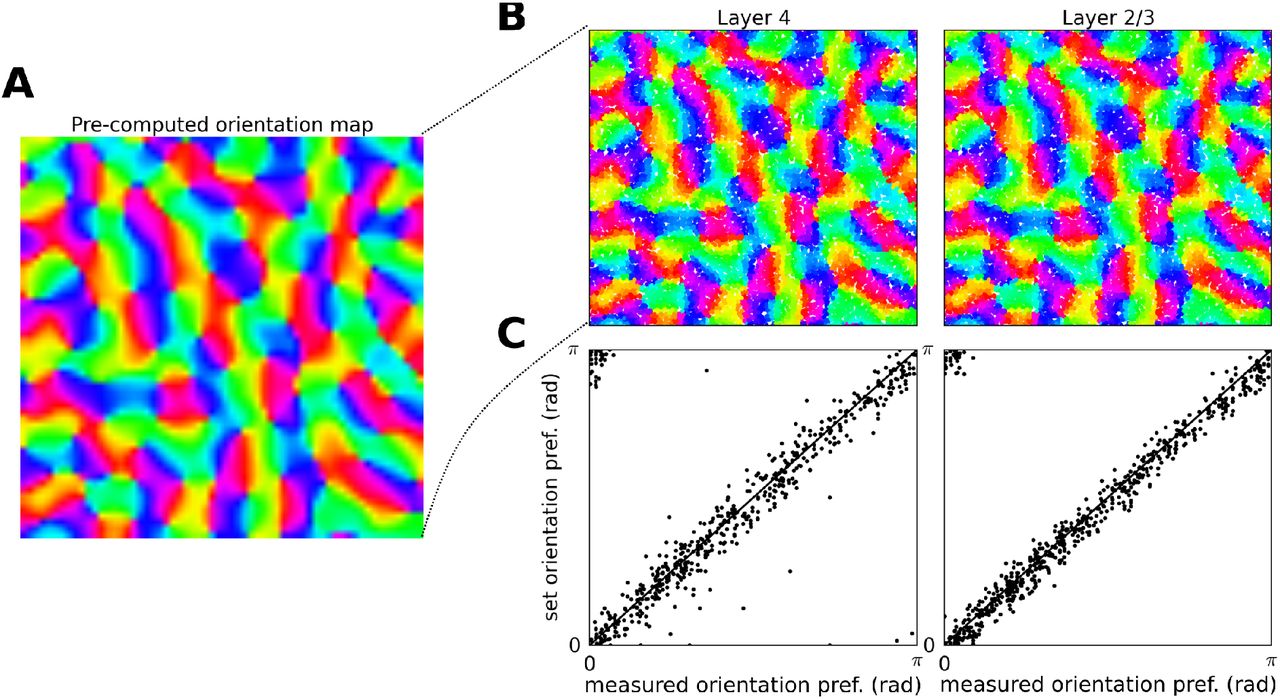
The induction of orientation maps in the model. (A) The precomputed orientation map that serves as a template based on which orientation of the cortico-thalamic connectivity of Layer 4 neurons is determined. (B) The orientation assigned to neurons in the two layers based on their position within the overlaid template orientation map. (C) The comparison between the orientation preference assigned to the neurons via the template (y axis) and the orientation preference measured using the sinusoidal grating protocol (y axis; see Section 2.4).
2.1.3 Cortico-cortical connectivity
The number of synaptic inputs per single neuron in primary visual cortex of cat has been estimated to be approximately 5800 [21]. While it is clear that a substantial portion of these synapses come from outside of V1, the exact number has not yet been established. A recent investigation by Stepanyants et al. [126] found that even for a cortical section 800 μm in diameter 76% of synapses come from outside of this region, while a rapid falloff of bouton density with radial distance from the soma has been demonstrated in cat V1 [32]. Furthermore, V1 receives direct input from a number of higher cortical areas including V2, V3, V4, V5/MT, MST, FEF, LIP and inferotemporal cortex, as well as other sub-cortical structures. It has been estimated that feedback from V2 alone accounts for as many as 6% and 8% of synapses in supra-granular layers of macaque and rat V1 respectively [30, 71]. Altogether it is reasonable to extrapolate from these numbers that as many as 50% of the synapses in layers 4 and 2/3 originate outside of the area.
The next important consideration when designing the basic connectivity parameters was the reliability of synaptic transmission in cortex. Cortical synapses have been shown to fail to transmit arriving action potentials, and even though this is a complex context-dependent phenomenon, past studies have shown that in cortex typically every other pre-synaptic action potential fails to evoke a post-synaptic potential [127, 4]. This is an important phenomenon as it implies a major change to the overall magnitude of synaptic input that can be expected to arrive into individual cells. It would, however, be computationally very expensive to explicitly model the synaptic failures, and so to account for the loss of synaptic drive due to the synaptic transmission failures we have factored it in to the number of simulated synapses per neuron. Thus, taking into account the average number of synaptic inputs (5800), and the estimates of the proportion of extra-areal input (50%) and of the failure rates of synaptic transmission (50%) we decided to model 1000 synaptic inputs per modeled excitatory cell. Inhibitory neurons receive 20% fewer synapses than excitatory neurons to account for their smaller size, but otherwise synapses are formed proportionally to the two cell type densities. 20% of synapses from Layer 4 cells are formed on the Layer 2/3 neurons. In addition Layer 4 cells receive 110 additional thalamo-cortical synapses [46]. The synapses are drawn probabilistically with replacement (with functional and geometrical biases described below), and the exact number of synapses according to numbers above is always established for each neuron, however because we allow formation of multiple synapses between neurons, the exact number of connected neurons and the effective strength of these connections is variable.
The geometry of the cortico-cortical connectivity is determined based on two main principles: the connection probability falls off with increasing cortical distance between neurons [31, 125, 32] (see Figure 1AB), and connections have a functionally specific bias; specifically they preferentially connect neurons with similar functional properties [32, 75]. The two principles are each expressed as a connection-probability density function, then multiplied and re-normalized to obtain the final connection probability profiles, from which the actual cortico-cortical synapses are drawn. The following two sections describe how the two probability density profiles of connectivity are obtained.
Finally, apart from the connectivity directly derived from experimental data, we also considered a direct feedback pathway from Layer 2/3 to Layer 4. Such direct connections from Layer 4 to Layer 2/3 are rare [25], however a strong feedback from Layer 2/3 reaching Layer 4 via layers 5 and 6 exists [25]. Since we found that closing of this strong cortico-cortical loop is important for correct expression of functional properties across the investigated layers, and because we decided not to explicitly model the sub-granular layers (see Section 2.1), we decided to instead model a direct Layer 2/3 to Layer 4 pathway. Since the parameters of this pathway cannot be directly estimated from experimental data, for the sake of simplicity, we have assumed it has the same geometry as the feed-forward Layer 4 to Layer 2/3 pathway (see following two sections).
2.1.4 Spatial extent of local intra-cortical connectivity
The exact parameters of the spatial extent of the model local connectivity, with the exception of excitatory lateral connections in Layer 2/3, were established based on a re-analysis of data from cat published in Stepanyants et al. [125]. Let  be the probability of potential connectivity (Figure 7 in Stepanyants et al. [125]), of a pre-synaptic neuron of type i ∈ (exc, inh} at cortical depth x to other post-synaptic neurons of type j at cortical depth y and lateral (radial) displacement z. We reduced the 3 dimensional matrix
  to a single spatial profile for each pair of layers and neural types (excitatory and inhibitory). This was done as follows. For each possible projection LpreTpre →LpostTpost where L corresponds to layers L ∈ (4, 2/3} and T corresponds to neuron type T ∈ (exc, inh} we did the following:
Select section of
 along the depth dimensions x,y corresponding to the pre-synaptic layer Lpre and post-synaptic layer Lpost.
Average the selected section of M along the the dimensions corresponding to pre- and post-synaptic layer depth, resulting in a vector representing the average lateral profile of potential connectivity of a neuron residing in layer Lpre to neurons residing in layer Lpost.
Normalize the resulting distance profile to obtain the probability density function.

To obtain a parametric representation of the distance connectivity profiles we fitted them with several probability distributions, including Gaussian, exponential and hyperbolic. We found that the best fits were obtained using the zero mean hyperbolic distribution:
 which was thus chosen as the parametric representation of the connectivity profiles. The resulting values of the parameters of the fitted hyperbolic distributions, for all combinations of pre- and post- synaptic layers and neuron types, which were used to generate the local connectivity distance dependent profiles in the model, can be found in Table 1.
Finally, the Stepanyants et al.[125] study reflects only the local connectivity, due to it depending on neural reconstruction in slices which cut off distal dendrites and axons further than 500 μm from the cell body, and also ignores any potential functional biases. In cat Layer 2/3, unlike in Layer 4, excitatory neurons send long-range axons up to several millimetres away, synapsing onto other excitatory and inhibitory cells 10, 32]. To account for this long-range connectivity in Layer 2/3 we follow the observation by Buz’as et al. [32], that the density of boutons across the cortical surface originating from the lateral connectivity of a small local population of stained Layer 2/3 neurons can be well approximated by the sum of two Gaussian distributions, one short range and isotropic and one long-range and orientation specific (see Section 2.1.5). Thus we model the lateral distribution of the Layer 2/3 excitatory connections as G(σs) + αG(σl), where G is a zero mean normal distribution, σs = 270μm and σl = 1000 μm are the short and long-range space constants chosen in-line with Buzas et al. [32], and α = 4 is the ratio between the short-range and long-range components. Another advantage of the Buzás et al. [32] model based approach to quantifying the later likelyhood of connectivity is that it also takes into account the functional biases that take place in Layer 2/3. How we incorporate these functional biases into our model is described in the following section.
2.1.5 Functionally specific connectivity
Unfortunately, the functional connectivity in V1 is still poorly understood. Experimental studies have shown that local connections in cat are diffuse, without a strong orientation bias [32], while long-range connections have a moderate bias towards iso-orientation configurations [32, 59]. Recent more detailed studies of local connectivity in mice have shown that local connections also have a weak bias towards connecting neurons with similar receptive field properties [75, 82]. Finally, the anti-phase relationship between excitatory and inhibitory conductances in cat V1 Simple cells in Layer 4 [88, 20] can be interpreted as further evidence for functionally specific inputs. Overall these results point to a weak tendency of excitatory neurons towards connecting nearby neurons of similar receptive field properties while this bias increases somewhat for more distant post-synaptic neurons.
Due to the lack of clarity and specificity of experimental data on the functional connectivity in V1, we use previously hypothesized schemes of functional connectivity and adapt them to be compatible with the above experimental findings. Within Layer 4 we assume push-pull connectivity [134] (see Figure 1E). For each pair of Layer 4 neurons the correlation c between their afferent RFs is calculated. The connectivity likelihood for a given pair of neurons is given by  where σ = 1.4 and μ =1 if the pre-synaptic neuron is excitatory or σ = 1.4 and μ = 1 if inhibitory.
In cat cortex excitatory neurons send long-range connections spanning up to 6mm along the cortical distance to both excitatory and inhibitory neurons, preferentially targeting those with similar orientation preference [32]. To reflect this connectivity in the model we define the connectivity likelihood between pairs of neurons in Layer 2/3 as  where the Δo is the difference between the orientation preference of the two neurons, and σ is set to 1.4. The connectivity likelihoods described above are renormalized for each neuron to obtain probability density functions. Note that only the long-range component of the Layer 2/3 model is multiplied by this functionally specific bias, while the short-range component remains non-specific (see Section 2.1.4). Overall this parametrization leads to only weak bias towards co-tuned connections in both simulated cortical layers.
2.1.6 Synapses
Synaptic inputs are modeled as transient conductance changes, with exponential decay with time-constant τe = 7.0 ms for excitatory synapses and τi = 11.0 ms for inhibitory synapses.
The relatively few studies that have examined in detail the strength of individual synapses in cortex have found that unitary synaptic strengths are generally weak (<2 nS), but broad ranges have been reported [66, 45]. While the overall specificity of the synaptic strength between pairs of neural types or layers remains unclear, a recent study in cat V1 has shown that synapses from excitatory onto inhibitory cells are considerably stronger than those targeting excitatory neurons [66, 45]. Reflecting these insufficient experimental constraints, the synaptic weights were selected to achieve an overall balance between excitation and inhibition that supports reasonable levels of both spontaneous and evoked activity, while being compatible with the limited physiological findings. Specifically, we set the intra-cortical excitatory-to-excitatory synapses to 0.375 nS and excitatory-to-inhibitory neurons to 0.675 nS, while all inhibitory synapses are set to 1.575 nS. Furthermore, the thalamocortical synapses were set to 1.2 nS, reflecting the findings that these synapses tend to be slightly larger [46] and more reliable [127] than their intra-cortical counterparts.
We have also modeled synaptic depression for thalamo-cortical, and excitatory cortico-cortical synapses [1] using the model of Markram et al. [87], while we do not model short term plasticity for inhibitory synapses as it is not well studied. For the thalamo-cortical synapses we assume parameters corresponding to weak depression similar to Banitt et al. and Kremkow et al. [18, 77] (U=0.75, τrec = 500 ms, τpsc = 7.0 ms and τfac = 0,ms). For the cortico-cortical excitatory synapses we assume stronger depression (U=0.75, τrec = 30 ms, τpsc = 7.0 ms and τfac = 0 ms), in line with Markram et al. [87].
2.1.7 Delays
We model two types of delays in the model circuitry. First are the delays due to the distance dependent propagation that are in the order of several tens of ms. These delays are important for lateral integration of information across multiple cortical columns. To reflect this, for all intra-cortical connectivity a distance-dependent delay with propagation constant of 0.3 ms-1 [27, 56, 70] was used, which corresponds to the slow propagation of action potentials along the intra-V1 (lateral) un-myelinated axons. The delays in the feedforward thalamo-cortical pathway are drawn from a uniform distribution within the (1.4,2.4) ms range. Second, Ohana et al. [96] have recently shown that delays of synaptic transmission in cat visual cortex are dependent on both pre- and post-synaptic neural type, with the notable feature of slow excitatory to excitatory and fast excitatory to inhibitory transmission. Distance-dependent axonal propagation delay is unlikely to explain these results as these experiments were performed in nearby neurons [96]. These pair-specific synaptic integration delays are in the order of only a few ms, but are important for local integration (within the same column) and for the precise timing of spike control by E/I interaction. Thus, as suggested by Ohana et al., we have included a constant additive factor in all synaptic delays, specifically 1.4 ms for excitatory to excitatory synapses, 0.5 ms for excitatory to inhibitory synapses, 1.0 ms for inhibitory to excitatory synapses and 1.4 ms for inhibitory to inhibitory synapses, in line with the quantitative observations by Ohana et al. [96]. We observed that the addition of this neuron-type-dependent delay factor improved the stability of the modeled cortical neural networks, reducing synchronous events during spontaneous activity. We hypothesized that this is due to the ability of inhibition to respond faster to any transient increase in activity in the network due to the shorter excitatory to inhibitory delay.
2.2 Input model
The input model described below corresponds to the whole retino-thalamic pathway. The cortical model corresponds to roughly 4.0 × 4.0° of visual field (Figure 1CF). To accommodate the full extents of RFs of neurons at the edges of the model, the LGN model corresponds to 5 × 5° of visual field. In the same manner, to accommodate the full extent of RFs of thalamic neurons the overall visual field from which the thalamic model receives input corresponds to 11 × 11°.
We do not explicitly model the retinal circuitry and use the widely-used center-surround model of receptive fields to simulate the responses of the LGN neurons (Figure 1C). The centers of both ON and OFF LGN neurons RFs are uniformly randomly distributed in the visual space, with density 100 neurons per square degree. Each LGN neuron has a spatiotemporal receptive field, with a difference-of-Gaussians spatial profile and a bi-phasic temporal profile defined by a difference-of-gamma-functions. Due to the relatively small region of visual space our model covers, we do not model the systematic changes in RF parameters with foveal eccentricity (nor, for the sake of simplicity, the natural cell-to-cell variance) and thus assume that all ON and OFF LGN neurons have identical parameters. The exact spatial and temporal parameters have been adopted from Allen and Freeman [5].
To obtain the spiking output of a given LGN neuron, the visual stimulus, sampled into 7ms frames, is convolved with its spatiotemporal receptive field. In addition, saturation of the LGN responses with respect to local contrast and luminance is modeled [102, 26]. For simplicity, the local luminance ll is calculated as the mean of luminance values and local contrast Ic as the standard deviation of the luminances within the RF of a given neuron. The response of the linear receptive field is separated into a DC (luminance) component rl and a contrast component rc. The saturation of the two components is modeled with two Naka-Rushton functions  and
and  respectively, where α is the gain and β is the saturation parameter of the corresponding component. The parameters α and β were empirically adjusted to obtain luminance and contrast response curves whose saturation point and level are within the range of those observed experimentally [102, 26].
The resulting luminance and contrast temporal traces are then summed and injected into integrate-and-fire neurons as a current, inducing stimulus dependent spiking responses. In addition to the stimulus-dependent drive, neurons are also injected with white noise current. The magnitude and variance of this noise is such that neurons fire ~ 10 spikes/s in the no stimulus condition [134]. This artificially elicited spontaneous discharge, calibrated to reproduce the experimentally observed spontaneous rates, corresponds to the combined effects of the dark discharge of the retina and any other potential intrinsic mechansism of spontaneous activity generation in the thalamus.
2.3 Stimulation protocols
One of the most important aspects of this study is the broad range of stimuli and associated experimental protocols with which the model was tested. In order to facilitate rigorous testing of future models, we publish the exact specifications of all stimuli and experimental protocol with ready to use implementations on the http://v1model.arkheia.org website and associated repositories.
Each stimulation protocol consists of a series of visual stimuli which are interleaved with 150ms of 50cd/m2 gray blank stimuli. In all experiments, with the exception of the size tuning protocol (see Section 2.3.3), we recorded spikes from 2337 randomly selected neurons, restricted to the central circular patch (radius of 1 mm) of the model to avoid contamination by potential edge-effects due to the finite simulated cortical area. Because the recording of intracellular signals at high temporal resolution for such a long stimulus set as presented in this work is extremely memory consuming, we recorded the membrane potential and excitatory and inhibitory conductances from a subset of 201 neurons confined to the central 0.2×0.2 mm patch of the simulated cortical space, and whose orientation preference (estimated as the expected orientation preference assigned to the neurons during model generation; see Section 2.1.5) was within 0.2 radians of horizontal.
The durations of all visual stimuli are aligned with the 7 ms frame duration at which the retino-thalamic model operates (see Section 2.2).
2.3.1 Spontaneous condition
Spontaneous activity was recorded during the presentation of a constant, blank stimulus of zero luminance lasting 130 seconds. In this condition, the visual stimulus does not contribute any input to the phenomenological models of LGN units (see Section 2.2), and thus corresponds to experimental recording in absolute darkness. Note however, that under these conditions the model LGN units still fire spikes at spontaneous rates observed experimentally [134], due to the additive Gaussian noise included in the LGN unit model (see Section 2.2), which corresponds to the combined effects of the dark discharge of the retina and any intrinsic mechanisms of spontaneous activity generation in the thalamus.
2.3.2 Drifting sinusoidal grating protocol
Sinusoidal gratings, which represent Fourier inputs in space and time, are the most common stimulus employed for characterizing functional properties of visual neurons [113]. They match the RF profile of the V1 neurons (when optimally parametrized) and thus provide a strong simultaneous feed-forward drive to a substantial portion of V1 neurons, leading to strong neural responses. They are thus ideal for parametric exploration of elementary functional properties of V1 neurons, such as orientation, contrast or frequency tuning.
The spatial and temporal frequency of the RFs of the modeled LGN neurons (see Section 2.1.2) and of the Gabor distribution template from which thalamo-cortical synapses were sampled were identical. An important consequence of this simplification is that it allowed us to efficiently execute protocols requiring drifting sinusoidal gratings. By employing a full-field stimulus with spatial frequency matching that of the Gabor template (0.8 Hz) and drifting at 2 Hz, we were in parallel stimulating all cortical neurons with a stimulus with optimal spatial frequency. Due to the lack of any direction preference mechanisms in the model, to further lessen the computational burden of the simulations, we varied the orientation of the gratings in 8 equal steps between 0 and 180 degrees. Each grating was shown 10 times for 2058 ms.
2.3.3 Size tuning protocol
A small stimulus can elicit a response from a neuron when presented in its RF, but by definition a neuron will not respond when the same stimulus is presented outside of the RF. However, when there is a stimulus in the RF that itself elicits a certain firing rate from the neuron, additional stimuli presented in the surrounding area can increase or decrease that firing rate. Such contextual effects in early vision are believed to underlie higher-level processes such as contour integration and figure-ground segregation.
Size tuning was measured using drifting sinusoidal gratings of optimal spatial and temporal frequency (see orientation tuning protocol for details), confined to an aperture of variable diameter, which were presented for 2058 ms and repeated 10 times. The orientation of the gratings was horizontal (0°) and the position was in the center of the simulated visual field. The aperture of the grating was gradually increased from 0° to 3° in 12 steps, each presentation lasting 2058 ms and repeated 10 times.
The center of the modeled cortical area was occupied by a horizontal orientation domain (see Figure 2). During the size tuning protocol we recorded from neurons in this central (horizontal) orientation domain and selected neurons whose receptive fields centers were within 0.1° from the center of the simulated visual field and whose orientation preference (determined by the orientation tuning protocol described above) was within 0.1 radians from horizontal. This setup allowed us to simultaneously determine the size t˃uning of the population of neurons reported here, with precision comparable to experimental studies, while greatly reducing the computational resources required for the simulation.
2.3.4 Natural images with simulated eye-movement protocol
We have replicated the natural image with simulated eye-movement protocol introduced by Baudot et al. [20]. This protocol emulates the global retinal flow experienced during the exploration of the natural environment, by simulating the retinal impact of visuomotor interaction by imposing shifts and drifts of a static natural scene which reproduce the kinematics of a realistic ocular scanpath [20]. We used the same image as in Baudot et al. [20], scaled to match the size of the simulated visual space. The image was moved within the visual field along a simulated path with statistics matching those of eye-movements in awake cats [20]. The same path as in Baudot et al. was used. Thus we have elicited movements across simulated receptive fields of the same spatial and temporal magnitude as in the experimental study. Presentation of the same resulting movie lasting 2058 ms was repeated 10 times.
2.4 Data analysis
Unless specified otherwise, all tuning curves in this study were calculated as the trial averaged mean firing rate during stimulation with the given stimulus and parameter value (i.e. orientation of sinusoidal grating). Spontaneous activity level was not subtracted, to make the tuning curves comparable to experimental studies [3, 38]. All analog signals (membrane potential, excitatory and inhibitory conductances) were recorded at 1 ms resolution to achieve managable data quantities, given the large number of neurons recorded and the length of the stimulation protocols.
To characterise the dynamical state of our network during the spontaneous condition at single cell and population level we have used two widely used descriptors [78, 47]. We calculate the irregularity of an individual neuron’s spike train as the coefficient of variation (CV) of its inter-spike-intervals (ISI):
 where Var corresponds to variance, and ˂ ˃ is the mean. To ensure accurate estimation of the irregularity we exclude neurons that fired fewer than 10 spikes during the duration of the spontaneous activity recording. For perfectly regular firing CVISI = 0, while a Poisson process yields CVISI equal to one. Following Kumar et al. [78] we set the threshold for irregular firing to CVISI > 0.8. We assess synchrony in our network by calculating the average cross-correlation (CC) of spike counts SCi SCj between disjoint pairs of all recorded neurons i, j.
 where Var is again variance and Cov is covariance of the spike count. The spike counts were calculated by counting the number of spikes within 10 ms bins.
In order to assess orientation tuning, we followed Nowak et al. [95] and calculated two complementary measures: the half width at half height (HWHH) and relative unselective response amplitude (RURA). To calculate HWHH we fitted the orientation tuning curves with a Gaussian function [3]:
 where R is the spiking response of the given neuron to a sinusoidal grating with orientation φ, φpref is the preferred orientation of the given neutron, σ is the width of the tuning, β is the baseline activity and α a scale factor. Low responding neurons (less then 1 spike/s at optimal orientation) were excluded from the analysis, as reliable curve fitting was not possible with the amount of recorded data. Furthermore, small minority of neurons (< 5%), for which reliable fit of Gaussian curve was not possible (MSE > 30% of the tuning curve variance) were also excluded from this analysis. HWHH was then calculated as
  RURA was calculated from the fitted Gaussian parameters according to the following equation [3]:

The modulation ratio (MR) of spike responses was computed as the ratio of the fundamental Fourier component F1 and DC component F0 of the neuron’s peri-stimulus time histogram (PSTH) in response to a drifting sinusoidal grating [122]. The PSTH was formed with 10 ms bins, and spontaneous activity was subtracted prior to MR calculation. The modulation ratio of the membrane potential was calculated analogously as the V1/V0 component ratio of the membrane potential after subtraction of its resting level.
Finally, we also examined the most common manifestation of surround modulation, the size tuning. To quantify the parameters of size tuning curves, following Wang et al. [138], we first fitted the data with the Supplementary Difference of Gaussians (3G) model defined as:
 where
where
 where r is the stimulus radius, Kc is the strength of the center, Ks is the strength of the suppressive surround, Kcs is the strength of the counter-suppressive surround (accounting for reduction of length suppression in the far periphery) and wx are the space constants of the corresponding terms. We then performed the following analysis on the fitted curves. First we determined the radii at which the peak summation occurs. The exact definition of this point in different studies varies slightly, the most important difference being that in some studies it has been computed directly from the raw tuning curves [118, 40, 72], whereas in others authors have first fitted the size tuning curve with models (of various kinds) and then derived these points from the fitted model parameters [69, 116, 129, 138]. Because the studies testing both approaches found very good agreement between the parameters derived in these two ways, we followed Wang et al. [138] and determined the parameters from the fitted curves. We have excluded low responding neurons (response of less then 2 spikes/s at the optimum size) from the analysis as we have observed poor curve fitting to these size tuning curves due to lack of data. We defined the summation peak δmax as the radius where maximum response is achieved before suppression sets in (we will also refer to this radius as the maximum facilitation radius (MFR)), suppression peak δmin as the radius where the minimum response is achieved across all aperture sizes greater than δmax, and the counter-suppression peak δcs as the radius where the maximum response is achieved across all aperture sizes greater than δmin. This in turn allows us to define the peak summation response Rmax, peak suppression response Rmin, and peak counter-suppression response Rcs as the neuron’s responses at the corresponding aperture sizes. We can then define the suppression index (SI) analogously to the experimental studies [138] as:
 and the counter-suppression index CSI as:
 Where
Where  and
and  are the summation peaks at low and high contrast, respectively.
The reliability and the precision of the responses were measured by fitting a Gaussian function to the mean cross-correlation across trials (Eq. 5) of the spiking responses, and of the sub-threshold membrane potential responses [20]. Spikes were removed from the membrane potential prior to the analysis, by replacing the membrane potential within a 5 ms window centred on each spike with the signal interpolated between the levels of membrane potential before and after the window. The reliability was then defined as the CC peak amplitude at time zero, and the temporal precision by the standard deviation of the Gaussian fit. Quantitative values in this article are expressed as mean ± SEM.
3 Results
The central goal of this study is to show that a single model of cat primary visual cortex, composed only of elements that do not contradict any existing experimental evidence, can reproduce an unprecedented range of previously identified phenomena, under a broad range of stimulation protocols. In order to present such a heterogeneous set of results in a clear manner, we organize the results such that each sub-section reviews the behavior of the model during a single stimulation protocol and compares it with experimental findings. All results presented here are based on data recorded in a single instantiation of the model.
3.1 Spontaneous activity
The model does not include any external sources of variability, with the exception of white noise current injection into LGN cells in order to induce their spontaneous firing at about 10 Hz, in line with recordings from visual thalamus [134]. This noise represents the combined effect of the dark discharge [39] in retina due to photonic noise or intrinsic properties of retinal ganglion cells [83, 52, 44, 115], and the intrinsic mechanisms generating ongoing activity in thalamus [111]. Consequently, since the thalamic inputs to Layer 4 neurons form only a small fraction of the modeled cortical synapses (in line with anatomy), the spontaneous activity (and variability in general) in the model is largely due to the internal dynamics of the model. This is an important factor for measurements that examine changes in cortical variability under different conditions such as those explored in Section 3.4.
In the spontaneous condition all modeled excitatory neuron populations fire irregularly (Figure 3A; Figure 4B: CV of ISI is above 0.8 in all layers) and asynchronously (Figure 3A; Figure 4C: the mean cross-correlation of the spike counts in excitatory populations is less then 0.01), with only occasional synchronized events, consistent with the spontaneous firing patterns of neurons in cortical slices [42, 119], awake animals [50, 81] and up-states in in vivo anesthetized preparations [50, 48]. The model exhibits slightly higher correlations between the spontaneous responses of inhibitory neurons then excitatory ones (Figure 3A; Figure 4C). Interestingly, higher synchrony among inhibitory neurons (as opposed to excitatory ones) has recently been reported in macaque cortex during slow wave sleep [80]. With the exception of Layer 2/3 inhibitory neurons, overall the spontaneous activity corresponds to the asynchronous irregular (AI) state previously observed in balanced randomly connected network models [137, 29, 136].

Spontaneous activity in modeled cortical layers. (A) Raster plot of spiking activity recorded for 5 ms of biological time in Layers 4 and 2/3 (from bottom to top; red: excitatory neurons, blue: inhibitory neurons). The relative number of spike trains shown corresponds to the relative number of neurons in the network (total of 400 neurons shown). (B-E) the membrane potential (black) and the excitatory (red) and inhibitory (blue) synaptic conductances of randomly selected neurons: (B) excitatory neuron in Layer 2/3; (C) inhibitory neuron in Layer 2/3 (C); (D) excitatory neuron in Layer 4; (E) inhibitory neuron in Layer 4.

Statistics of spontaneous activity in the simulated network. (A-F) Six measures of spontaneous activity for excitatory (black bars) and inhibitory (white bars) neural populations in the two modelled cortical layers. Error bars report standard deviation.z (A-C) Statistics of the spiking activity of the 4 modeled cortical populations based on spike trains recorded for 130 s. (A) Mean single-unit firing rates. (B) Irregularity of single-unit spike trains quantified by the coefficient of variation of the inter-spike intervals. (C) Synchrony of multi-unit spiking activity quantified as the mean correlation coefficient between the PSTH (bin size 10ms) of all pairs of recorded neurons in a given population. (D-F) Mean values of intracellular variables: membrane potential (D); excitatory (E) and inhibitory (F) synaptic conductances. (G) The distribution of firing rates (black points) in Layer 4 and 2/3 excitatory and inhibitory neurons is well fitted by a log-normal distribution with matching mean and variance (gray line; left-column). The log-normal distribution appears as a normal distribution on a semi-logarithmic scale. The data is better fit by a log-normal (gray line) than by an exponential (dashed line) distribution (right-column; log-log scale).
The mean firing rates differ considerably between cell types (Figure 3A). We observe higher mean spontaneous rates in inhibitory populations than in excitatory populations, in line with experimental evidence [28, 128], while the spontaneous firing rates of the majority of excitatory neurons are low (<2Hz), as observed in cat V1 [91, 19] (Figure 4A). The firing rates of individual neurons can differ substantially from the population mean, as shown by the population histograms in Figure 4G. In all four cortical populations, the firing rates closely follow log-normal distributions (Figure 4G), a phenomenon previously shown in several cortical areas and species [67, 33].
We also investigated intracellular responses of the model neurons in the spontaneous state. The mean resting membrane potential of neurons is close to −70mV, as observed in in vivo cat V1 recordings [92]. As shown in Figures 3B and 4EF, the excitatory synaptic conductances recorded in model neurons during spontaneous activity are low (0.95 nS, averaged across all layers) and close to the levels observed experimentally in cat V1 (~1 nS; layer origin not known) [92]. The inhibitory conductance during spontaneous activity was 5.1 nS when averaged across all layers and neural types, also in a very good agreement with the value of 4.9 nS reported in in vivo cat V1 recordings [92]. The balance of excitation and inhibition during spontaneous condition in the model is thus in a very good agreement with in-vivo data in cat V1 [92]. These levels of conductance are in stark contrast to those in most balanced random network models of spontaneous activity, in which the global synaptic conductance tends to be orders of magnitude higher [136, 78]. Overall the model exhibits a spontaneous state with balanced excitatory and inhibitory inputs well matched with cat V1 for both extra- and intracellular signals, without the need for any unrealistic external sources of variability. This represents an advance over previous models of V1 and over dedicated models of spontaneous activity, and enables a self-consistent exploration of stimulus-driven changes in variability in subsequent analysis (see Section 3.4).
3.2 Responses to drifting sinusoidal gratings
Figure 5 shows the responses of representative excitatory and inhibitory cells from both modeled cortical layers to multiple trials of optimally and cross-oriented oriented sinusoidal gratings of optimal spatial frequency, drifting at 2 Hz. As shown in Figure 5A (bottom panel), the membrane potential of the Layer 4 excitatory cell follows the sinusoidal modulation of the grating luminance—characteristic of Simple cells [92]—but remains largely unmodulated and below threshold during the cross-oriented condition. The sinusoidal shape of the membrane potential trace is the result of the excitatory and inhibitory synaptic conductances being mutually in anti-phase (Figure 5A middle panel), as a result of the push-pull connectivity in model Layer 4. The trial-averaged excitatory and inhibitory synaptic conductances are low (mean value across recorded neurons 5.64 nS and 29.4 nS respectively), comparable with observations in cat V1 [92, 20]. As a result of the sinusoidal subthreshold dynamics, the spikes are generated in a phasic manner aligned to the upswings of the membrane potential, while the cross-oriented grating does not elicit significant depolarization so that the membrane potential remains below threshold and consequently no spikes are generated.

Responses of representative excitatory (A,C) and inhibitory (B,D) neurons from Layer 4 (A,B) and Layer 2/3 (C,D) to 10 trials of drifting gratings of optimal (left) and cross-oriented (right) orientations. For all neurons, the top panel is a spike raster plot, each line corresponding to a single trial. The middle panel shows the incoming synaptic excitatory (red) and inhibitory (blue) conductances and the bottom panel shows the membrane potential (thin lines: single trials; thick lines: mean). Stimulus onset is at time zero.
The spiking response of the inhibitory cells in Layer 4 (Figure 5B) is similar, but the smaller number of incoming synapses (see Section 2.1.6) leads to slightly lower mean input conductances (mean value across recorded neurons; excitation: 5.0 nS, inhibition: 22.7 nS), while the stronger excitatory to inhibitory synapses (see Section 2.1.6) mean that the conductance balance is shifted towards stronger relative excitation during visual stimulation, thus leading to higher overall firing rates (see Section 3.2.1).
Unlike the phasic response of Layer 4 cells, both excitatory and inhibitory cells in Layer 2/3 show steady depolarization in response to an optimally orientated grating, similar to non-linear Complex cells (Figure 5CD). The mean excitatory and inhibitory conductances are 3.7 nS and 21.3 nS respectively, within the range of conductance levels observed experimentally [92, 20].
3.2.1 Orientation tuning of spike response
We next examined the responses of the model to different orientations of the sinusoidal grating at two different contrasts. As illustrated in Figure 6A, in both cortical layers most excitatory and inhibitory units had realistically shaped tuning curves [3].

Orientation tuning properties of excitatory and inhibitory neurons in Layers 4 and 2/3. (A) Orientation tuning curves calculated as the mean firing rate of the neuron at the given orientation. The large tuning curves on the left represent the mean of centered orientation tuning curves across all the measured neurons of the given type. The smaller tuning curves on the right correspond to randomly selected single neurons. (B) Half-width-at-half-height (HWHH) at 100% vs 10% contrast. (C) The distribution of HWHH measured at 100% contrast across the four modeled cortical populations. (D) The distribution of relative unselective response amplitude (RURA) measured at 100% contrast across the four modeled cortical populations.
The mean tuning widths of excitatory and inhibitory neurons in Layer 4 and excitatory and inhibitory neurons in Layer 2/3 measured as half-width-at-half-height (HWHH) were 23.8°, 34.0°, 24.6° and 32.4° respectively (see Figure 6C), which is within the range of tuning widths in cat V1 outlined by experimental studies [95, 38, 53]. Even though some sub-groups of inhibitory neurons have been shown to be broadly tuned to orientation [95], on average inhibitory neurons are well tuned [38, 95] just as in our model. In both modelled layers inhibitory neurons were more broadly tuned (mean HWHH across all inhibitory neurons 32.4°) than the excitatory ones (mean HWHH across all excitatory neurons 24.1°), which is in a very good quantitative agreement with values measured by Nowak et al. [95] (mean HWHH of regular spiking neurons 23.4°, and fast spiking 31.9°).
It is important to note that because the HWHH measure does not take into account the unselective response amplitude, cells that respond substantially above the spontaneous rate at all orientations, but where this unselective response is topped by a narrow peak, will yield low HWHH. To address this concern Novak et al. [95] also calculated the relative unselective response amplitude (RURA; see Methods), and showed that while if viewed through the HWHH measure inhibitory neurons are only moderately more broadly tuned then excitatory ones, the RURA of inhibitory neurons is much broader. We have repeated this analysis in our model, and as can be seen in Figure 6 C and D, the difference between excitatory and inhibitory neurons on the RURA measure is indeed much more pronounced (0.53% in excitatory vs 15.3% in inhibitory neurons), and in good quantitative agreement with values reported in Novak et al. [95] (mean for regularly spiking neurons 2.5% and fast spiking neurons neurons 18.1%).
As evidenced by the mean and single neuron orientation tuning curves shown in 6A, most excitatory and inhibitory units in the model cortical Layer 4 and 2/3 exhibit contrast invariance of orientation tuning width, which is further confirmed by comparing the HWHH of the tuning curves at low and high contrast (Figure 6B: most points lie close to the identity line). On average we observe very minor broadening of the tuning curves at high contrast, and it is more pronounced in inhibitory neurons: the mean HWHH differences between low and high contrasts is 0.8° (excitatory, Layer 4), 1.51° (inhibitory, Layer 4), 0.14° (excitatory, Layer 2/3), and 0.83° (inhibitory, Layer 2/3). Such minor broadening has been observed experimentally in simple cells in cat V1 (0.3°; layer origin nor neural type not known [53]).
Overall, the orientation tuning in our model is in very good qualitative and quantitative agreement with experimental data, with both excitatory and inhibitory neurons exhibiting sharp and contrast-invariant orientation tuning across all modelled layers, in contrast to many previous modelling studies that relied on untuned inhibition, or broad contrast-dependent inhibition [134, 79, 41].
3.2.2 Orientation tuning of sub-threshold signals
To better understand the mechanisms of orientation tuning in the model, we investigated the tuning of the membrane potential and the excitatory and inhibitory synaptic conductances. An essential mechanism responsible for orientation tuning in this model is the push-pull connectivity bias in Layer 4. In theory, a cell with a pure push-pull mechanism with perfectly balanced excitation and inhibition should exhibit purely linear (Simple cell) behavior, where orientation tuning is solely driven by the luminance modulation of the drifting grating, and the mean membrane potential should remain at resting (spontaneous) level at all orientations. In order to assess to what extent this idealized scheme is true in this model, we have examined the DC (F0) and first harmonic (F1) components of the analog signals, and plotted the mean orientation tuning curves across the different neural types and layers in Figure 7.

Orientation tuning of membrane potential and excitatory and inhibitory conductances of excitatory and inhibitory neurons in Layer 4 and 2/3. Each row shows a different layer and neural type, see labels. Orientation tuning curves of: (A) F0 component of membrane potential; (B) F1 component of membrane potential; (C) F0 component of excitatory synaptic conductance; (D) F1 component of excitatory synaptic conductance; (E) F0 component of inhibitory synaptic conductance; (F) F1 component of inhibitory synaptic conductance. Low contrast: 10% (blue line), high contrast: 100% (black line).
The orientation tuning of membrane potential in Layer 4 (in both excitatory and inhibitory neurons) is dominated by the F1 component, in line with the presence of strong push-pull mechanisms in this model layer (Figure 7 B). Layer 4 cells also have significant tuning of the mean membrane potential, but of smaller magnitude (Figure 7 A). The F0 components of the membrane potential show noticeable broadening at higher contrast, consistent with observations by Finn et al. [53] that, unlike the spiking response, the orientation tuning width of the membrane potential is not contrast independent. In Layer 2/3 the magnitude of the Vm components is reversed: the magnitude of the F0 component of the membrane potential is stronger than the F1 component. This is consistent with the lack of phase specific connectivity in this model layer, and explains the predominance of Complex cells in this layer, as will be further elaborated in Figure 8. Furthermore, for excitatory cells in Layer 2/3, unlike in those in Layer 4, the F0 of the membrane potential exhibits contrast invariance of tuning width.

Modulation ratio of excitatory cells in the model. (A) Histogram of modulation ratios calculated from the PSTH over recorded excitatory cells in Layer 4 (first row), Layer 2/3 (second row) and pooled across both layers. (B) as in (A) but modulation ratio calculated from the membrane potential after subtraction of background level. (C) As in A but the histograms are of the absolute value of the F0 component of the membrane potential. (D) As in C but for the F1 component of the membrane potential. (E) The relationship between the modulation ratio calculated from PSTH and from membrane potential. In the pooled plots and in panel E cells classified as simple are marked white and as complex are marked black.
How does the interplay between excitation and inhibition lead to the observed membrane potential tuning characteristics? To answer this question, in Figure 7C-F we plot the orientation tuning curves of the F0 and
F1 components of excitatory (C,D) and inhibitory (E,F) synaptic conductances. In Layer 4, the most obvious difference is that in comparison to the tuning of membrane potential, the F0 component of both excitatory and inhibitory conductances dominates the F1 component. The weaker F0 component of the membrane potential in Layer 4 neurons is thus due to the cancellation between the excitatory and inhibitory F0 components, while the F1 component of the membrane potential orientation tuning remains strong, as such cancellation between excitatory and inhibitory conductances does not occur due to the half period phase shift between them (see Figure 5A,B). In Layer 2/3 both F0 and F1 of excitatory and inhibitory conductances in both excitatory and inhibitory neurons are well tuned, but the F0 components dominate in magnitude the F1 components both for excitatory and inhibitory conductances and in both neural types.
Overall we observe that for all layers and cell types both F0 and F1 components of membrane potential and conductances exhibit orientation tuning of varying degree, consistent with observations made by Anderson et al. [7]. The contrast invariance in orientation tuning arises as a complex interplay between excitation and inhibition, differs between layers and neural types, and in the model Layer 4 is consistent with engagement of push-pull mechanism [134]. However additional enhancement of activity is present due to the recurrent facilitatory dynamics among neurons of similar orientation, that goes beyond the predictions of the push-pull model, as evidenced by the presence of tuning in the F0 components of the membrane potential of layer 4 neurons.
3.2.3 Simple and Complex cell types
Next we examined the classification of the cells into Simple and Complex. In line with the behavior of the representative model neurons shown in Figure 5, the modulation ratio computed from the PSTH of most neurons in Layer 4 is greater than one, which classifies them as Simple cells (see Figure 8A). The same measure for most neurons in Layer 2/3 is less than one, classifying them as Complex cells (see Figure 8A). This laminar bias towards different modulation ratios is in line with previous experimental evidence [65]. When pooled across the two layers the histogram of modulation ratios forms a bimodal distribution (see Figure 8A), as observed experimentally [106].
Unlike for the PSTH, the modulation ratios computed from the membrane potential Vm (with the resting potential subtracted) when pooled across the two modeled cortical layers form a unimodal distribution (see Figure 8B) with a peak at zero, which is in line with experimental evidence in cat [106]. However, the range of modulation ratios of Vm is higher in the model compared to cat V1, due to a greater number of cells that behave nearly linearly in Vm. When the modulation ratios calculated from PSTH and membrane potential are plotted against each other (Figure 8E), a characteristic hyperbolic relationship is revealed, in line with the observations of Priebe et al. [106]. However, when analyzing the F0 and F1 component of the membrane potential individually, greater differences from the experimental data are revealed. The distributions of both F0 and F1 Vm components in both layers are considerably narrower than shown in cat [106] (Figure 8C,D). When pooled across layers this lower variation of the F0 and F1 components leads to a bimodal distribution, unlike in the experimental data.
Overall the behavior of the model is a good qualitative match to the cat data on Simple and Complex neuron classes, and is in agreement with related previous computational models, but several discrepancies arise when a quantitative comparison is made. The main discrepancy is that the distributions of the F0 and F1 components of membrane potential 8C,D) are narrower in both modelled layers, than experimentally observed [106], which in the case of the F1 component of membrane potential leads to a bimodal distribution when pooled across the two modeled layers, unlike the data of Priebe et al. [106]. It should be noted though, that in that study, the histogram showing the F1 component of membrane potential, more than 90% of data is in the first 3 bars, and so it is not possible to say if ‘zooming’ into the lower range of values, which encompasses an absolute majority of cells, might not reveal a separation between Simple and Complex cells in this measure. The overall lower range of values for the F0 and F1 measures in the model, compared to cat data, could be due to intrinsic regularities present in the model, such as identical physiological parameters among all cells of the same cell type, or limited variability of the ratio of afferent and recurrent inputs to model Layer 4 neurons, or completely phase un-specific connectivity from Layer 4 to 2/3. Unfortunately, the values of these parameters in cat V1 have not yet been investigated, but it is reasonable to expect some variation, and introducing such variability in the model could thus rectify these discrepancies.
3.3 Size tuning
We have also examined the most well studied manifestation of contextual modulation, size tuning, whereby one presents a drifting sine grating confined to an aperture of increasing radius, and records the response as a function of the aperture radius. Figure 9 shows the size tuning properties of excitatory cells in both modeled cortical layers. Most excitatory neurons in both cortical layers show surround suppression (Figure 9A-D), however we observe a diversity of tuning patterns. In the first row of Figure 9 we can see an example of Layer 4 cells with prototypical size tuning properties, including the expansion of facilitation radius at low contrast [138, 129]. On the other hand, in the second row of Figure 9 we show an example of a Layer 4 cell that exhibits only weak suppression and does not exhibit the contrast dependent shift of facilitation radius. Neurons in Layer 2/3 also express classical size tuning effects as exemplified in the third row of Figure 9.

Size tuning in excitatory neurons. The first three rows show size tuning in three example model neurons. Top row is a typical Layer 4 cell with strong size tuning, second row shows an example of Layer 4 cells that does not exhibit size tuning, and the third row shows a typical Layer 2/3 cell. (A) The size tuning curve of trial-averaged spiking responses. Dots are measured responses, line is fitted size tuning curve. (B) The size tuning curve of trial-averaged mean membrane potential. (C) The size tuning curves of trial-averaged mean excitatory (red) and inhibitory (blue) synaptic conductances. Data shown for low and high contrast conditions: (A-B) low-contrast (10%) condition is blue, high-contrast (100%) condition is black; (C) low-contrast (10%) condition is un-saturated, high-contrast (100%) condition is saturated; (D-H) Scatterplots of size-tuning measures. Arrows mark means after pooling across layers. White (empty in H) dots correspond to individual Layer 4 neurons and black (full in H) dots correspond to Layer 2/3 neurons. (D) The suppression index of spike responses at low vs. high contrast. (E) The counter-suppression index of spike responses at low vs. high contrast. (F) The suppression index vs. the counter-suppression index at high contrast. (G) the maximum facilitation radius at low vs. high contrast. (H) The suppression index of excitatory (red) and inhibitory (blue) synaptic conductances at low vs. high contrast.
The degree of the suppression varies widely in both cortical layers (Figure 9D). Overall the suppression is stronger in Layer 2/3 (mean suppression index (SI) at high contrast: 0.34 ± 0.009) than in Layer 4 (mean SI at high contrast: 0.24 ± 0. 012). These values are well within the range observed experimentally in cat V1 (i.e. 0.16 [129], 0.35 [97], 0.44 [138] and 0.47 [2]; cells pooled across all cortical layers). Stronger suppression in Layer 2/3 than in Layer 4 was observed in two of the three studies ([97, 2]) while Wang et al. [138] did not observe a statistically significant difference in SI between Layer 4 and 2/3. Finally, in line with Wang et al., we observe a decrease of suppression at low contrast (mean SI at low contrast: 0.23 ± 0.012 Layer 4 and 0. 28 ± 0.016 Layer 2/3).
A more recent finding regarding surround suppression is that many neurons do not exhibit monotonic suppression after reaching their classical RF size, but after a certain radius their responses partially recover from the suppression [138]. This phenomenon has been named counter-suppression. We observe this in a substantial subset of model neurons across both modelled layers (Figure 9E). When quantifying the magnitude of this counter-suppression as the CSI index, Wang et al. [138] found that it tends to be stronger at low contrast than at high contrast, and that the suppresion index SI is almost always stronger than the CSI. In our model we find that on average the CSI index at low contrast is moderately stronger (mean CSI at low contrast: 0.05 ± 0.008 Layer 4 and 0.07 ± 0.01 Layer 2/3) than at high contrast (mean CSI at low contrast: 0. 04 ± 0.005 Layer 4 and 0.052 ± 0.007 Layer 2/3), which is qualitatively in line with Wang et al., although we observe a less robust effect in the model, i.e. smaller a proportion of neurons follow the trend, than in cat. We do also observe the stronger SI over CSI in an absolute majority of model neurons, in very good accordance with Wang et al..
We also observe increase of the the maximum facilitation radius (MFR) at lower contrast (Figure 9G; mean MFR at high contrast: 1.0 ± 0.02 Layer 4 and 0.94 ± 0.009 Layer 2/3 vs. mean MFR at low contrast: 1.19 ± 0.018 Layer 4 and 1.09 ± 0.044 Layer 2/3) (see Figure 9G). This contrast dependent change of ~20% is slightly lower than in Wang et al. [138] and Tailby et al. [129] who found increases of 33% and 36% respectively in cat V1. On average, both excitatory and inhibitory conductances are size tuned at both low and high contrast and in both simulated cortical layers (Figure 9H), in line with experimental evidence [8, 101].
3.4 Responses to natural images with simulated eye-movements
Next we probed the model with a stimulus consisting of a natural scene animated with simulated eye-movements, as described in quantitative intra-cellular study of Baudot et al. [20]. As can be seen in Figure 10B, the natural image stimulus elicits a highly repeatable response, both at the level of spikes and at the level of sub-threshold responses, unlike the response to presentation of a drifting grating which is only locked to the slow temporal frequency of the luminance modulation, in accordance with findings by Baudot et al.[20] in cat V1.

Trial to trial reliability of responses to a natural image with simulated eye movements (NI) and to drifting sinusoidal gratings (DG). (A) The response of a randomly sampled excitatory neuron in model Layer 4 to the DG stimulus. The top panel shows the spike raster histogram, the middle panel shows the incoming synaptic excitatory (red) and inhibitory (blue) conductances. The bottom panel shows the membrane potential. The thick lines show the mean of the analog signals over the 10 trials. (B) As (A), but for the NI stimulus. (C-F) Cross-correlation across trials for spikes (top) and subthreshold membrane potential activity (bottom), in response to DG and NI stimuli. The reliability is given by the peak amplitude at time zero, and the temporal precision by the standard deviation of the Gaussian fit to the cross-correlation. (C) Results averaged across all recorded excitatory neurons in model Layer 4. (D) Results averaged across all recorded excitatory neurons in model Layer 2/3. (E) Results averaged across all recorded neurons pooled across the two model layers. (F) The experimental data from Baudot et al. [20]. Note that in that study two additional stimuli were also presented (dense noise : blue line; grating with simulated eye-movements : green line) that we have not used in this study. (G-I) The inverse of the stimulus-locked time-averaged standard deviation of membrane potential (1/SD) across trials, averaged across cells, relative to the value for ongoing activity. (G) Experimental results in cat [20]. (H) Results averaged across all recorded excitatory neurons in model Layer 4. (I) Results averaged across all recorded excitatory neurons in model Layer 2/3. in established anatomical and physiological data, which expresses an unprecedented range of V1 properties (see Table 2).
To further investigate the response precision and reliability of the model neurons we computed the crosscorrelation between trials both of the spiking responses and of the membrane potential responses. The reliability is given by the peak amplitude of the cross-correlation (a) at time zero, and the temporal precision by the standard deviation of the Gaussian fit (σ) [20]. As shown in Figure 10C,D, for the spiking response (top), both for model Layer 4 and Layer 2/3 neurons, the cross-correlation has a higher peak and is narrower for the natural-image-with-eye-movement (NI) stimulus (Layer 4: α=0.1, σ=6.7; Layer 2/3: a=0.03, σ=8.2), than for drifting sinusoidal gratings (Layer 4: a=0.05, σ=61; Layer 2/3: a=0.0079,σ=60), in line with the experimental results in Baudot et al. [20] (see Figure 10F).
For the membrane potential (Figure 10C,D bottom) the same relationship holds except that for Layer 4 neurons the peak (and thus the reliability) for gratings is slightly lower than for natural images (Layer 4 natural images: a=0.37, σ=11; Layer 2/3 natural images: a=0.12, σ=8.7; Layer 4 gratings: a=0.4, σ=91; Layer 2/3 gratings: a=0.02, σ=46), unlike the observations in Baudot et al. [20] (Figure 10F), where the reliability is higher for the NI stimulus for both spikes and membrane potential. However, note that in Baudot et al.[20] the results are pooled across neurons of all layers, and the same treatment of our data produces higher reliability for natural images also in the model, in line with Baudot et al. [20] (Figure 10E). Therefore this can be considered a prediction of our model, specifically that the reliability of membrane potential responses for Simple (or Layer 4) cells alone is higher for drifting gratings than for NI stimuli.
Furthermore, Baudot et al. [20] found that relative to the trial-to-trial variability of membrane potential during spontaneous activity, the variability of Vm during DG stimulation increases, while it decreases during NI stimulation (Figure 10G). We have performed the same analysis on the model, the results of which are shown in Figure 10(HI). In both model layers we observe an increase of stimulus-locked variance (calculated as the inverse of the stimulus-locked time-averaged standard deviation across trials, and expressed as a percentage relative to the value for ongoing activity) for DG (97 ± 0.68% in Layer 4 and 96 ± 0.23% in Layer 2/3) but a decrease of stimulus-locked variance for the NI condition (122 ± 0.99% in Layer 4 and 104 ± 0.35% in Layer 2/3), in line with Baudot et al. [20].
4 Discussion
Despite the wealth of existing models of early visual processing we still lack a single coherent explanation for how the various identified computations coexist within the multiplicity constraints of the underlying cortical neural substrate. Past models of primary visual cortex failed to exploit the full breadth of constraints imposed by the numerous existing experimental studies. The multiplicity of constraints and their impact on diversity across cells may be a key factor accounting for the difficulty of associating canonical circuit patterns to specific computations relative to a given functional feature (i.e. orientation preference, natural scene encoding). It is likely that the principle of ‘optimal coding’ might be misleading when focusing on any one single processing property and confounding cells across layers. Each cell has to realize in its own way the same operation in different intra-cortical constraint contexts (compare for instance Layer 4 and 2/3, or regions close or far from pinwheel centers)
Here we have for the first time approached this problem with a systematic integrative data-driven computational modeling methodology, constructing a single spiking model of primary visual cortex firmly grounded
4.1 Knowledge integration
We show here that a single set of experimentally supported principles of cortical connectivity—(i) weakly orientation-biased thalamic inputs to Layer 4 neurons, (ii) local, weakly push-pull-biased intra-Layer 4 connections, and (iii) local and long range weakly orientation-specific intra-Layer 2/3 connections—can give rise, within the same model instantiation, to a majority of the most salient V1 computations. The model demonstrates sharp orientation tuning curves across neural layers and neural types, whose width does not change with contrast and quantitatively matches the experimentally observed differences between layers and neural types (Figure 6). We also show that not only the spiking output of the model but also all the subthreshold signals are orientation tuned, in line with experimental evidence (Figure 7). We show how predominantly Simple cells arise in Layer 4 as a consequence of the direct (albeit weak) phase-specific thalamic inputs and the weak bias towards push-pull connectivity among the Layer 4 cells, and how predominantly Complex cells arise in Layer 2/3 due to phase-nonspecific pooling from Layer 4. When the simpleness/complexness is quantified as the modulation ratio of the spiking output, the typical bimodal distribution arises, whereas the modulation ratio of membrane potential remains unimodally distributed in line with in vivo data (Figure 8).
The same simulated neural substrate that provides an accurate account of these V1 properties typically attributed to the classical receptive field captures also the processing attributed to the extra-classical RF, i.e. surround modulation. Specifically, we show that cells in all modeled layers exhibit size tuning with magnitudes of suppression and optimal diameters that match physiological data (Figure 9). The model also correctly captures the contrast dependent changes of these measures (Figure 9). When analyzed at the subthreshold level, the model also replicates the recently discovered size tuning of both excitatory and inhibitory conductances (Figure 9), demonstrating that the model can capture the highly non-linear dynamical nature of cortical computations.
The ability of the model to accurately describe the stimulus-driven neural dynamics of primary visual cortex is not only confined to artificial stimuli. When stimulated with a movie with naturalistic spatio-temporal statistics, the model replicates the recently-identified stimulus dependent changes to the precision and reliability of spiking responses (Figure 10), as well as the pattern of stimulus-dependent changes to the trial-to-trial variability of membrane potential (Figure 10). Finally all these stimulus evoked properties of the model are underlaid by a resting state that is quantitatively in agreement with physiological data (Figure 4).
4.2 Novelty and predictions
It is this original convergence of the five key integrative principles in a single study - (i) the multitude of anatomical constraints respected, (ii) the multiplicity of neural signals (synaptic, single unit) and integration levels (conductance, neuronal, columns) examined, (iii) the multiplicity of the stimulation protocols tested, (iv) the diversity of functional phenomena explained, and (v) the multiplicity of spatial and temporal scales examined - that constitutes the central novel contribution of this study. While the model can thus explain many of the V1 phenomena previously studied in isolation, it also offers mechanistic explanations for previously unexplored features of V1 processing, and several testable predictions. To the best of our knowledge, this model represents the first self-consistent description of the background activity regime in primary visual cortex that is both quantitatively accurate at supra- and, crucially, also sub-threshold levels, and self-consistent in the sense that it does not rely on any ad hoc hand-tuned direct external noise input to cortical neurons.
In turn, this accurate capture of spontaneous dynamics allows the model to show, for the first time, how the trial-to-trial variability of membrane potential of V1 neurons can increase (with respect to the spontaneous state) during drifting grating stimulation and decrease during naturalistic movie stimulation [20]. The self-consistent treatment of spontaneous activity (with no artificial external intra-cortical source), allows the trial-to-trial variability in the model to be primarily shaped by the intra-cortical interactions during both the spontaneous and stimulus driven activity. This is an advance over a recent model of a V1 column that explained the precision and reliability changes between the grating and naturalistic stimuli at the spiking level but did not reproduce the stimulus-dependent variability effect at the level of membrane potential [77]. This was due to the inclusion of substantial random spiking input directly into cortical neurons, which induced substantial stimulus-independent variability of the membrane potential, overriding the internally generated components. These differences point out the importance of simultaneously capturing within a single model the cortical processing under multiple stimulation conditions and at different levels of signal integration, to be able to fully describe its operation.
Another unique feature of our model is its ability to accurately capture the emergence of orientation tuning in primary visual cortex at both supra- and sub-threshold levels. Electrophysiological experiments in V1 impose important constraints on the principles of generation of orientation tuning in V1. Specifically, they imply that (i) orientation tuning is sharp across all granular and supra-granular cortical layers [38], (ii) the inhibitory neurons are only moderately more broadly tuned than excitatory ones [94, 38], and (iii) both DC and F1 components of spikes, membrane potential and excitatory and inhibitory conductances tend to be tuned to the cell’s preferred orientation [7] (although inhibitory conductance shows greater diversity of orientation tuning relative to spike-based preference [91, 92, 55]). Many past models have only explored the orientation tuning of spiking responses [68, 24, 37, 107] and relied on either broadly tuned (or un-tuned) inhibition [123, 134, 79, 41] or inhibition tuned to the orthogonal orientation [121, 43] which is in contradiction with inhibitory conductances tuned to preferred orientation [7]. Few past models have been consistent with the constraint of sharply tuned responses of inhibitory cells and of inhibitory input tuned to the preferred orientation [112], and to the best of our knowledge no model has yet demonstrated the orientation tuning of both the DC and F1 components of all the sub-threshold signals. This model obeys all these experimentally imposed constraints, and thus represents the first mechanistic explanation of orientation tuning generation in primary visual cortex that is fully consistent with this range of physiological data.
In addition to the broad range of properties of V1 processing reproduced in this study, the model also goes beyond existing data, offering a number of testable predictions:
Layer- and cell-type-specific differences in the parameters of spontaneous activity. While a number of basic parameters of the spontaneous activity in V1 have been reported, and are in good agreement with the presented model (see Section 3.1), data on the layer and cell type specific differences are missing. Among others, we predict that the spontaneous rates of inhibitory neurons in V1 are about six times that of the excitatory ones, and that the spontaneous rates in Layer 2/3 are lower than that of neurons in Layer 4 (Figure 4). We also predict greater synchrony among the inhibitory neurons.
Distribution of modulation ratios of spiking and membrane-potential responses to sinusoidal gratings individually in Layer 4 and 2/3. Only distributions that pool across cortical layers have been reported in cat so far (Figure 8).
Layer-specific and cell-type-specific differences in stimulus dependent changes to the precision and reliability of spiking and trial-to-trial variance of membrane potential. We predict that Layer 4 cells do not have lower precision when responding to sinusoidal gratings as opposed to when responding to animated natural images, however this relationship appears, as predicted by Baudot et al. [20], once cells are pooled across Layer 4 and 2/3.
Near contrast invariance of inhibitory neurons with only minor broadening at high-contrast.
Layer-specific differences in sub-threshold signal tuning. It has been shown that both the F0 and F1 components of sub-threshold signals are selective to preferred orientation in most cells [7, 91], in accordance with our model. But sufficient data have not been collected to verify the specific differences in tuning width of the different components between layers and cell types that are predicted by this model.
While most parameters of the model have been chosen based on existing experimental findings, several important testable assumptions had to be made due to lack of existing data:
(a) The sharpness of functional specificity of excitatory cortico-cortical connections within Layer 4 neurons.
(b) The ratio between the overall strength of excitatory to excitatory vs excitatory to inhibitory pathways that effectively sets the overall ratio between excitation and inhibition in the model.
(c) We have assumed here, that the strong intra-areal feedback pathway from Layer 2/3 via Layer 5 and 6 back to Layer 4 can, at least from the point of view of intra-areal processing, be simplified as a direct feedback from Layer 2/3 to Layer 4. Future combinations of anatomical and functional studies and modeling can reveal how close this assumption corresponds to the biological reality.
4.3 Other models of orientation tuning in V1
Genesis of orientation selectivity (i.e. tuning and preference) and emergence of the ON-OFF layout of Simple and Complex receptive fields are the two features of V1 function that were in the past by far the most common target of computational studies, leading to dozens of alternative explanations of these V1 features. In an attempt to systematize the field, V1 models tend to be categorized according to two main properties: (1) the degree of cortical connectivity: so-called ‘feed-forward’ vs ‘recurrent’ models and (2) the selectivity of the cortical inhibition in the orientation and phase domains. It is important to emphasize that the existing V1 models cannot be separated into discrete categories, and most of their features are shared, while even along the dimensions of distinction the differences often are a matter of degree rather than category [131]. Briefly, in the ‘feed-forward’ models [134, 68, 51] orientation tuning is largely determined by the thalamo-cortical (feed-forward) pathway, and the cortical machinery, while still present, has only a minor influence on the shape of the tuning. This is reflected in the connectivity of the models, which tends to be dominated by a strong and sharply orientation tuned thalamo-cortical pathway. In contrast, the recurrent models [24, 24, 49] assume that the thalamic input to V1 is poorly tuned and weak, while strong intra-cortical interactions drive the shaping of orientation tuning. With respect to inhibition, the defining features are its orientation tuning width (relative to excitation), its presence or absence at orthogonal orientations, and its relationship to the phase of the stimulus.
As we have pointed out above, this categorization is highly oversimplified, ignoring a plethora of implementation details and, most importantly, the fact that models can in principle exist anywhere along the continuum of these parameter axes and combine features that are typically associated with different classes (e.g. one can study models with sharply tuned feed-forward input but with dominant intra-cortical interactions). In this study we have side-stepped any attempt to cast the model into this standard classification system, and rather followed solely the existing anatomical and physiological evidence to determine its architecture. Indeed, as we will show in the following, the model does not fit into any of the standard classes but rather resides somewhere in between. The orientation tuning in the model is driven by thalamo-cortical connections following a Gabor profile with a low aspect ratio of its subregions (2.5), and the thalamo-cortical pathway constitutes a minor fraction of the synaptic input to Layer 4 cells (~ 5%). These features would assign the model to the recurrent category [131]. On the other hand, the dominating intra-cortical connections in Layer 4 are biased towards a push-pull organization, which has been typically assumed in feed-forward models [134, 131], but - based on recent experimental evidence [32, 75] - this functional bias is much weaker than in previous computational studies. In Layer 2/3 the connections are not phase specific, but are biased towards the same orientation [32], in line with the recurrent model category.
Note, however, that this connectivity scheme is not arbitrary. The push-pull scheme in Layer 4 is motivated by the fact that it has been shown in multiple studies that in Simple cells in Layer 4, the excitatory and inhibitory conductances are in anti-phase [88, 92, 20], and such correlation based connectivity is the only plausible explanation for this phenomenon to date. On the other hand, the phase non-specificity in Layer 2/3 is the consequence of the lack of phase-selectivity of Complex cells that dominate in this layer. This connectivity scheme is thus consistent with all the current experimental findings, and can be viewed as a self-consistent end-product of Hebbian-like plasticity (anti-Hebbian in the case of inhibitory synapses) and stimulus driven development in V1 [11, 74].
In the model Layer 4 the inhibition is phase specific, and as a consequence of the low functional specificity of the intra-cortical connections it is broad and thus present also at orthogonal orientations. Crucially, as we show in Figure 6, the resulting orientation tuning at the spiking level is sharp, comparable to that of excitatory neurons, in line with experimental evidence [38]. This shows that even in a model with weak and weakly orientation-tuned afferent input and broadly tuned intra-cortical inhibitory input, the resulting orientation tuning of inhibitory neurons can be sharp, in line with experimental evidence [38, 7, 91]. The fact that the model behaves as neither a standard feed-forward nor recurrent model can also be seen from examining the sub-threshold signals. In classical feed-forward models the DC component of the feed-forward excitatory input is canceled by the DC component of the inhibition [134, 131]. It is the F1 component of the membrane potential (which remains due to the anti-phase inhibition) that induces the orientation tuning (and the contrast invariance of tuning width) of the neurons. As we show in Figure 7, our model exhibits orientation tuning of the DC components of both excitatory and inhibitory conductances and also of the membrane potential, in line with the boosting of mean response at preferred orientations typical of recurrent models (and in line with experimental evidence). At the same time, the push-pull connectivity remains an important factor shaping the orientation tuning and its contrast invariance in the model, as evidenced by the dominance of the F1 components in Simple cells (Figure 7). This shows that the different strategies of generating orientation tuning typically associated with recurrent and feed-forward models can co-exist within the same neural circuit, while being consistent with a broader range of physiological findings, in turn offering another example of the benefits of the data-driven integrative approach.
Finally, recently an alternative purely feed-forward explanation of orientation tuning, that does not at all rely on intra-cortical interactions, has been proposed by Finn et al. [53]. The two key mechanisms involved in this model are: (1) the influence of an expansive non-linearity that governs the relationship between the mean and variance of the membrane potential and the spike rate, and (2) the contrast dependence of the feed-forward synaptic thalamic input [114]. This modeling study shows that in principle contrast invariant orientation tuning can arise without intra-cortical interactions, but what remains to be understood is the expansive non-linearity implemented in the neural substrate. One possibility is that an effective expansive non-linearity can be induced by the non-linear recurrent dynamics of cortical circuitry. So, although the formulation of the model [53] looks feed-forward, the assumed non-linearities may absorb recurrent contributions. Furthermore, it is not clear how can the Finn et al. model also explain other V1 phenomena such as the fact that the modulation of the membrane potential is dominated by inhibition [64, 7, 91, 92], or more generally the generation of the anti-phase relationship between inhibition and excitation, as well as contextual modulation. Ultimately, the principles described by Finn et al.. can be yet another mechanism contributing (together with those already described above) to the orientation tuning in V1. Of the required mechanisms, the expansive non-linearity is already present in our model, while recurrent interactions, such as those in our model, can further contribute to the effective expansive nature of the neuron’s transfer function. Thus, addition of the contrast dependent variability of the thalamic inputs described by Finn et al. [53, 114] would be sufficient to induce these alternative orientation tuning processes in our modeling paradigm.
4.4 Other large-scale models of orientation tuning
In the previous section we focused on models that have targeted orientation tuning as the primary subject of investigation, and that generally ignored other aspects of V1 processing as well as details of its large-scale topological organization. Far fewer computational studies have pursued such broader goals. Somers et al. [124] investigated a topologically-organized model of V1, which incorporated excitatory connections that dominated at short distances, and inhibitory ones that dominated at medium distances. There is, however, little anatomical evidence for such a spatial arrangement [125]. Evidence for such direct medium-range inhibitory connections is lacking, however the wider spread of the lateral inhibitory kernel may be the functional disynaptic expression of long distance horizontal excitatory connectivity impinging on local (short-range) inhibitory neurons. Indeed, the excitatory neurons in the model also sent long-range connections. All connection probabilities were biased towards co-oriented neurons, but ignored the phase specificity of their targets, which implies that the model was not able to replicate the phase-specific relationship between excitatory and inhibitory conductances. Beyond this assertion it is difficult to assess how the model matched physiological measures at sub-threshold levels as only the spiking output was analyzed and the model did not consider the spontaneous activity regime. Functionally, similarly to this study, the Somers et al. model was able to demonstrate the emergence of contrast-invariant orientation tuning, and contrast dependence of size tuning, but none of the other features of V1 processing were examined.
Another similar pair of modeling studies was performed by Wielaard et al. [141, 142] who also considered a large region of topologically organized cortex. Unlike Somers et al. [124] and this study, these modeling studies did not consider long-range cortical interactions, and in contrast to Somers et al. [124] they assumed that short-range exitatory connections have longer range than the inhibitory connections, which is more in line with the anatomical data [125] also used in our study. Finally Wielaard et al. also did not consider any functional specificity of intra-cortical interactions. Wielaard et al. demonstrate the emergence of both Simple and Complex cell types, determined by the ratio of thalamic and cortical input. They also show how a bimodal distribution of modulation ratios at the level of spiking can emerge despite unimodally distributed modulation ratios of membrane potential. Furthermore, they show how such an only-locally-connected cortical model can explain the emergence of size tuning, quantitatively well matching experimental results. Interestingly, the authors do not demonstrate some of the more classical properties of V1 neurons, such as sharp mean orientation tuning (the limited data presented indicate a predominance of poorly tuned cells) or its contrast invariance. As in the present study, Wielaard et al. perform sub-threshold analysis of the model, analyzing how size tuning of spike responses emerges as a function of excitatory and inhibitory conductances and resulting membrane potential dynamics. Similar to our model, Wielaard et al. demonstrate that the size tuning arises as a complex dynamic interplay between excitation and inhibition, whereby both conductances exhibit reduction at large stimulus sizes. Unfortunately Wielaard et. al. do not assess the sub-threshold signals quantitatively, or characterize the background activity in the model. Finally, orientation specificity of the surround in their model was also not tested and no other stimuli beyond drifting sinusoidal gratings were probed.
Probably the most comprehensive V1 modeling effort prior to this one is a series of modeling studies [34, 130, 108] summarized in Rangan et al. [109], architecturally very similar to the Wielaard et al. models [142, 141]. In multiple related models the authors have demonstrated a range of V1 properties in both spontaneous and evoked states, including a fluctuation-driven spontaneous activity regime characterized by low firing rates [34], emergence of sharply tuned Simple and Complex cell types with a bimodally distributed modulation ratio of spike responses and unimodally distributed modulation ratio of membrane potential [130], and approximate contrast invariance of orientation tuning. The study also demonstrated two features of V1 computation not examined in the our model: the spontaneous activity dynamics that are correlated with the intrinsic orientation organization of cortex [34], and the spatio-temporal patterns of cortical activity in response to a line-motion illusion stimulus, which are similar to those observed in analogous voltage sensitive dye imaging experiments [108]. Unlike in the present study, neither the contextual modulation nor naturalistic stimulation were explored in these models, nor was a detailed quantitative account of their sub-threshold behavior provided. Finally, while all the models summarized in Rangan et al. [109] share a common architecture, it is not clear whether all these studies used identical parametrization of the models, and consequently if all these features could be achieved within a single model instance. This is particularly crucial, given that in our experience even minor changes to critical parameters in such highly recurrent models can have a strong influence on the expression of the features examined.
A study from the Allen Institute just came out that follows a comprehensive data-driven approach [15]. Independently of the size of datasets constraining the two models, the 5 major differences between present study and Arkhipov et al. [15] are the species and preparation state choice, the level of refinement in biophysical and morphological neuronal description, the nature of the electrophysiological recordings to test the model, the level of refinement in the control of sensory statistics and investigation (or not) of optogenetic manipulation. In our study we model the cat V1 in the anesthetized state, whereas Arkhipov et al. constrained their model using data from awake mice. The advantage of the anesthetized condition is that a lot more data on visual system has been collected over the years and is thus availabel for constraining of our model (now and in future), and that the better stimulus control during experiments and reduced non-visually driven input into V1 due to animal behavior allows for better dissection of visually driven processes. On the other hand, the awake conditions allows the study of the neural substrate of visually guided behavior, and eliminates potential misinterpretation of anesthesia induced artefact’s in data as normal visual processing. Another advantage of the Arkhipov et al. [15] study is that they incorporated greater biological detail by also considering neural morphology and 10 active conductances at the soma. On the other hand, the Arkhipov et al. model is tested against extra-cellular multi-electrode recordings in contrast to the intra-cellular data constraining our model also at the level of membrane potential and conductances. The authors employed a relatively broad set of test protocols, including spontaneous activity, grating stimuli, and natural movies. Whereas the choice of the classic Orson Welles movie for Arkhipov et al. study was motivated by search for high contrast natural scenes to raise the detectability of calcium transients, the choice of natural scene animation in the cat experiments that were targeted in our study was dictated by our will to reproduce in the most realistic fashion the retinal flow produced by cat eye-movements during natural exploration of natural scenes (Baudot et al. [20], Supplementary). A welcomed novel addition in the Arkhipov et al. study is also the examination of the model against data under optogenetic manipulation.
Arkhipov et al. demonstrated a good match of the model against data on number of properties including realistic magnitude of response to gratings, orientation selectivity, amplification of LGN responses, prominence of gamma oscillations, and log-normal distributions of firing rates. On the other hand an important advantage of the present study compared to Arkhipov et al. [15] is that we have focused more on the more complex functional properties, such as size tuning or trial-to-trial precision, and offered more systematic characterization of the examined properties in the model with respect to experimental data. Interestingly, Arkhipov et al. also compared the biophysically detailed model with an integrate-and-fire version constructed at a similar level of detail as the present study, and showed that qualitatively the simplified model remains a very good match to in vivo data, although they do point out some measures where the quantitative match suffered. This is a welcome justification for the approach presented here. Finally, we would like to point out that the targeting of mouse V1 in Arkhipov et al. [15] has both advantages and disadvantages. On one hand, the rodent does not seem to be a choice model for vision when it is obviously more adapted (in the ecological sense) for the haptic modality or the study of multi-modal integration [58]. The mouse V1 still remains less well characterized, especially functionally, than cat or macaque, and major differences in both anatomical and functional organization in comparison with ‘higher’ mammals have been shown. On the other hand, advances in optogenetics are rapidly expanding our knowledge of mouse V1 and the semi-industrialization of data acquisition in this species generates datasets that are particularly suitable for the comprehensive data-driven approaches that we and Arkhipov et al. champion. Ultimately, we believe having parallel investigations in different strategic animal models (mouse, cat, macaque) and at different levels of detail is desirable, and, rather than using a single species model where optogenetic tools best apply, a generalization of comparative studies to species where valuable functional descriptions have been obtained will shed more light on the mode of cortical processing across different species [57].
Another broader treatment of V1 computations has been provided in the recent study by Rubin et al. [112]. Unlike the other studies discussed in this section, it is based around a more simplified, firing-rate network model of cortex that is set up to operate as an inhibition stabilized network. The model represents a retinotopically organized patch of Layer 2/3, taking into account also the presence of orientation maps, but all the up-stream processing is simplified away. The model also makes the common, anatomically unsupported, assumption of longer range excitatory to inhibitory than excitatory-to-excitatory connections, which the authors claim is essential for a number of the demonstrated properties. The strength of this model is that, despite its relative simplicity, it is upon further simplification amenable to more in-depth analysis, it can demonstrate an impressive range of cortical processing effects, chiefly corresponding to two types of effects: normalization and surround suppression (see Table 2 for full list). The study, however, seeks only to capture the experimental results qualitatively, thus leaving the possibility that a more accurate explanation of the biological system is not feasible within this framework. It also avoids examination of some of the more basic properties such as orientation tuning or the resting regime of the network. With respect to the latter, the authors in fact point out in their discussion section that, under the assumption of the spontaneous regime, their model would always operate in the supra-linear regime, which would in turn preclude the model explaining the contrast dependent switching from facilitatory to suppressive integration. This is in line with our experience, that the spontaneous regime represents a very important constraint for the model dynamics, and can thus exclude many operating regimes in the evoked state as possible explanations for biological data. Being a firing-rate based model, the Rubin et al. study also lacks the ability to capture trial-to-trial variability related cortical processes, which (as we also demonstrate here) play important role in several features of cortical computation [78, 130, 20].
Finally, recently Chariker et al. [41] have also made the case for a more comprehensive approach to the computational study of primary visual cortex, presenting a model that is, similarly to the present study, firmly grounded in anatomical data. The number of properties demonstrated in the model is, however, still limited, not exceeding the range presented in the series of studies of Wielaard et al. [142, 141] or those summarized in Rangan et al. [34, 130, 108, 109], although it is important to emphasize that, unlike those other model series, Chariker et al. [41] explicitly demonstrate that all the claimed properties can emerge in a single model instance. The authors do not probe the model with any stimulus other than the ubiquitous drifting sinusoidal grating. The quantitative analysis of the model is limited: for example the orientation tuning in the model seems to be too broad, while characterization of the spontaneous state is missing. The authors do not investigate basic properties such as contrast invariance of orientation tuning, which, judging by the elevated firing of the example V1 cells in the cross-oriented condition, is missing. Not least in importance, the analysis of model properties at the sub-threshold level is not presented at all.
Overall we believe the present study represents an significant advance towards providing a comprehensive integrative treatment of primary visual cortex. Together with the technological advances in building such complex integrative models in a modular manner, which we have fully shared with the community [13], and the principled approach to sharing the results and all relevant metadata from this study (http://v1model.arkheia.org) as well as the associated tools [12], we provide the most advanced platform for future long-term systematic incremental integrative research into primary visual cortex and beyond.
4.5 Modeling choices and future work
The key motivation of this study is our contention that computational neuroscience needs an increased focus on pluripotent models of brain function. To this end, we have presented here a large-scale spiking point-neuron model of primary visual cortex. This model surpasses any previous V1 model in terms of the range of functional and structural features of primary visual cortex that it covers (Table 2). However, it still addresses only a fraction of known V1 properties. As stated in the Introduction, we hope this is just the first entry in a long-term systematic effort in building a single comprehensive model of V1 and beyond. Why do we, however, believe this is the right first entry? First, V1 is one of the most well studied cortical areas, with a breadth of existing experimental and computational studies, and is thus particularly suited to, and in need of, knowledge consolidation. Second, the choice of the level of modeling detailed employed here is what we consider a middle ground, where we neither engage low-level details such as neural morphology or detailed channel dynamics, nor opt for high-level approximations such as mean field approaches. The advantages of this middle ground approach are the following: (i) most of the experimental findings specific to V1 processing are naturally represented at this level of detail, thus allowing us to directly address most of the most salient features of V1 computation; (ii) this level of detail enables a clear, direct link between the underlying neural substrate and V1 function, without necessitating the inclusion of computationally challenging anatomical or dynamical features (e.g. detailed morphology, channel kinetics etc.); (iii) as a platform for future research it facilitates integration across scales by allowing direct expansion of the modeling scope in both directions, towards low-level features (by simply replacing the neural models with more detailed approximations of ones choice), and high-level features (by expanding the model towards further cortical layers, other cortical and sub-cortical areas and measurements of associated functional phenomena).
Validation of visual cortex models with respect to experimentally observed functional properties. A tick means that the model gives a qualitatively good match to experimental findings. A cross means that the model gives a response which is qualitatively different from experimental findings. Empty spaces mean that the model was not tested for the property, and it is not possible with certainty to conclude from the corresponding paper that the model does or does not match corresponding experimental data. We have restricted this table to models of cat or macaque V1, as the two species represent the two major animal models in vision while their anatomical and functional similarity allows for straightforward comparison.
In this study we have opted to model neurons as exponential integrate-and-fire units with conductance-based synapses [54]. This choice had several motivations. First, as we have demonstrated here, a number of important characteristics of V1 computations are manifested at the precision level of single spikes and/or trial-to-trial variance of sub-threshold neural signals (a necessary condition for validating or challenging predictions of theoretical frameworks linked to the spike-timing coding hypothesis), and such quantities do not have a direct representation in firing-rate based models. We also show here how the dynamics of sub-threshold signals, including the excitatory and inhibitory synaptic conductances, provide an important means for constraining the model, which thus excludes usage of current-based synapse models. The particular choice of the exponential variant of the conductance-based integrate-and-fire scheme was motivated by our observations that the variable effective threshold in this neural model secures more stable asynchronous behavior than the simpler fixed-threshold variants. Second, we chose not to pursue more detailed representations of single neuron dynamics, such as a full morphological representation or channel kinetics, for two main reasons: (i) the neuron counts necessitated by the cortical area considered in this study, and length of the stimulation paradigms targeted in this study would make simulations with such detailed neural models nearly intractable on currently availabel computing resources, (ii) the understanding of the role of such low-level neural features in cortical computation is still in its relative infancy, especially in terms of direct consequences on the most salient computations performed in V1 that we have targeted here, thus rendering the need for knowledge integration at this level much less important, and (iii) lack of sufficient detailed reconstructions of neurons in cat V1 with associated intracellular functional data [17] and lack of detailed characterization of ion channel kinetics and ion channel dendritic distributions in cat.
Structurally, the model makes four main simplifications with respect to the biological neural substrate: (i) the omission of layers 5 and 6 [133, 132], (ii) omission of the cortico-thalamic feedback pathway [139, 120], (iii) omission of the feedback from higher cortical areas [9, 30], and (iv) reduction of neural dynamics to only two types (excitatory and inhibitory) [143, 94]. The infra-granular layers have been omitted because their role in cortical processing is much less understood than that of the granular and supra-granular layers and there is thus much less data availabel for constraining their model. Furthermore, they are believed to be largely involved in sub-cortical projections and feedback projection from higher level cortical areas [84], which are another two features not considered here. The constituents of the cortico-thalamic pathways (i.e. PGN and the arborization of Layer 6 axons in LGN and PGN) are very poorly studied, and the evidence on the functional role of the cortico-thalamic feedback is also very sparse, thus also not lending itself as a first candidate for integrative treatment.
The cortico-cortical feedback, mediated partly by long-distance supra-granular connections, represents a particularly difficult challenge for modeling, as it in principle requires some form of treatment of all the numerous higher-cortical areas that send feedback to V1, while relying on a relatively sparse set of findings on the anatomy, physiology and computational principles of these feedback structures. The cortical neurons do not form a homogeneous population; rather anatomical, physiological and genetic studies have revealed a plethora of sub-types, especially among the inhibitory population [86, 16]. Due to the recent methodological advances in selective targeting of these different subtypes in physiological experiments, the different roles they play in cortical processing [104, 63] are starting to be uncovered. This mapping out of the neural sub-type characteristics is, however, still in an early stage, and is largely confined to the mouse animal model, without a clear understanding of how these findings will translate to cortical processing in higher mammals. There are strong arguments in favor of major architectural genomic differences in the visual cortex connectome between mouse and higher mammals. Big Data approaches by the Allen Institute in the mouse and human brain building large-scale cellular resolution gene profiles in the neocortex show species-specific differences in molecular signatures. In particular, they attest to a quantitative shift from down regulation of gene expression in Layer 5 to upregulation in Layer 3, indicative of a transfer from cortico-subcortical to more predominant cortico-cortical communications from the mouse to the human brain [145]. Undoubtedly, continuing systematic exploration of the neural sub-type specificities, especially if successfully translated into higher mammalian models, would provide an invaluable trove of constraints to be integrated within the integrative modeling paradigm proposed here.
Ultimately, the main reason for omission of these important structural features was to restrict this initial study to a manageable (both computationally and conceptually) level of complexity; the model, however, still proved to be a rich environment for exploration, sufficient for explaining the majority of the most salient properties of V1 computation. We would like to emphasize that even though we argue here for an integrative, comprehensive treatment of the neural systems under study, we acknowledge that this has to be an incremental process. All these omissions would be natural candidates for the next steps of the integrative research program initiated in this study. To that end, as the next step, work is in progress in our group to integrate corticothalamic feedback into this modeling paradigm [14].
The variability in our model can be attributed to two principal sources: the stochastic nature of thalamocortical and cortico-cortical connectivity wiring-pattern generation, and the simplistic simulation of intrinsic thalamic variability by a white-noise source. Even though, as we show, these sources are sufficient to explain a considerable amount of variability in a number of measures of cortical function (e.g. see Figure 10), we have also encountered several cases where the model exhibits lower variability than generally identified experimentally (e.g. the magnitudes of F0 and F1 components of the membrane potential due to stimulation with sinusoidal gratings; Figure 8). It is reasonable to expect that additional sources of variability exist. For example, while the exact set of post-synaptic neurons in each of the model’s projections is determined stochastically (within the confines of the connectivity generation rules outlined in Section 2.1.5), the number of them generated per neuron (i.e. the overall strength of the given projection into the neuron) is fixed. This effectively means that every neuron within each modelled layer will receive exactly the same proportion of input from the different projections. It is reasonable to assume that in animal cortex the relative strength of inputs from the different projections in individual neurons will be considerably more variable.
Another aspect of the model that negatively influences its variability are the regularities in the generation of its architecture. For example we assume all thalamic neurons (at a given visuotopic eccentricity) have equally large receptive fields and we assume fixed size, spatial frequency and aspect ratio of the templates from which afferent connectivity (and thus ‘afferent’ RF) of Layer 4 V1 neurons is generated. We also assume that both the ON and OFF channels are of equal strength, even though recent electro-physiological investigations revealed the dominance of the OFF pathway and systematic variations of the ON-OFF pattern of RF following the orientation maps [76, 140]. All these structural parameters are known to have substantial biological variability [73, 38, 110]. They are the result of developmental processes, whether intrinsic or stimulus driven, which both have stochastic components, but more importantly likely generate features of cortical organization more broadly adapted to processing of visual stimuli that are not accounted for in our model (and presumably some or even most have not even been discovered yet). Unfortunately, quantitative estimates of these various sources of variability are not currently availabel. Our modeling paradigm could be used in the future to formulate predictions for these values by evaluating which additional sources of variability and of what magnitude could account for the experimental observations. An alternative intriguing possibility would be adoption of a hybrid scheme, whereby some of the variability due to the developmental processes would be directly simulated in dedicated adaptive models (e.g. see [11, 74]), and then transplanted into the detailed spiking modeling paradigm for more thorough examination.
In this study we have chosen to model only a weak bias of cortical neurons towards connecting to co-tuned neighbors. It should however be noted that the effective functional bias is in fact higher, due to the functional organization of receptive field properties along the modeled cortical surface. The presence of functional maps along the cortical surface implies that even connections from a given neuron that would be drawn based on a functionally nonspecific rule would more likely synapse onto neurons preferring the same orientation. Finally, let us point out that it is likely that the functional specificity of intra-cortical connections in V1 is significantly higher than the level indicated by the limited number of experimental studies that have been conducted, but the unaccounted-for specificity is due to functional biases yet to be investigated, or biases to functional properties that have not been discovered yet. Such functional wiring specificities can have genetic but also epigenetic origins, whereby specific salient features of the sensory-motor experience of each individual are imprinted via Hebbian-like learning processes (especially during the early post-natal development) onto the cortical wiring. Therefore, the parameters of functionally specificity of connections in the model should be viewed as a combination of true level of randomness in cortical connectivity with an unbiased representation of the yet to be identified specificities.
Acknowledgements
This research has received funding from the Centre National de la Recherche Scientifique, Paris-Saclay IDEX (NeuroSaclay), the French National Research Agency (Complex-V1), the European Union’s Seventh Framework Program under grant agreements 269921 (BrainScaleS) and 604102 (Human Brain Project), and through project CZ.02.2.69/0.0/0.0/17_050/0008466 Improvement of internationalization in the field of research and development at Charles University.
References
- [1].↵
- [2].↵
- [3].↵
- [4].↵
- [5].↵
- [6].↵
- [7].↵
- [8].↵
- [9].↵
- [10].↵
- [11].↵
- [12].↵
- [13].↵
- [14].↵
- [15].↵
- [16].↵
- [17].↵
- [18].↵
- [19].↵
- [20].↵
- [21].↵
- [22].↵
- [23].↵
- [24].↵
- [25].↵
- [26].↵
- [27].↵
- [28].↵
- [29].↵
- [30].↵
- [31].↵
- [32].↵
- [33].↵
- [34].↵
- [35].↵
- [36].↵
- [37].↵
- [38].↵
- [39].↵
- [40].↵
- [41].↵
- [42].↵
- [43].↵
- [44].↵
- [45].↵
- [46].↵
- [47].↵
- [48].↵
- [49].↵
- [50].↵
- [51].↵
- [52].↵
- [53].↵
- [54].↵
- [55].↵
- [56].↵
- [57].↵
- [58].↵
- [59].↵
- [60].↵
- [61].↵
- [62].↵
- [63].↵
- [64].↵
- [65].↵
- [66].↵
- [67].↵
- [68].↵
- [69].↵
- [70].↵
- [71].↵
- [72].↵
- [73].↵
- [74].↵
- [75].↵
- [76].↵
- [77].↵
- [78].↵
- [79].↵
- [80].↵
- [81].↵
- [82].↵
- [83].↵
- [84].↵
- [85].↵
- [86].↵
- [87].↵
- [88].↵
- [89].↵
- [90].↵
- [91].↵
- [92].↵
- [93].↵
- [94].↵
- [95].↵
- [96].↵
- [97].↵
- [98].↵
- [99].↵
- [100].↵
- [101].↵
- [102].↵
- [103].↵
- [104].↵
- [105].↵
- [106].↵
- [107].↵
- [108].↵
- [109].↵
- [110].↵
- [111].↵
- [112].↵
- [113].↵
- [114].↵
- [115].↵
- [116].↵
- [117].↵
- [118].↵
- [119].↵
- [120].↵
- [121].↵
- [122].↵
- [123].↵
- [124].↵
- [125].↵
- [126].↵
- [127].↵
- [128].↵
- [129].↵
- [130].↵
- [131].↵
- [132].↵
- [133].↵
- [134].↵
- [135].↵
- [136].↵
- [137].↵
- [138].↵
- [139].↵
- [140].↵
- [141].↵
- [142].↵
- [143].↵
- [144].↵
- [145].↵
- [146].↵
- [147].↵


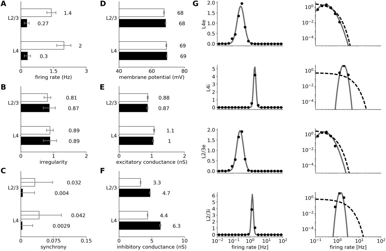
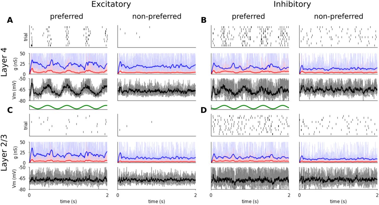
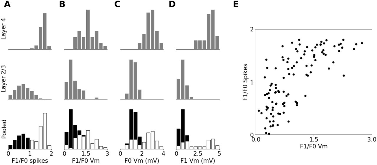
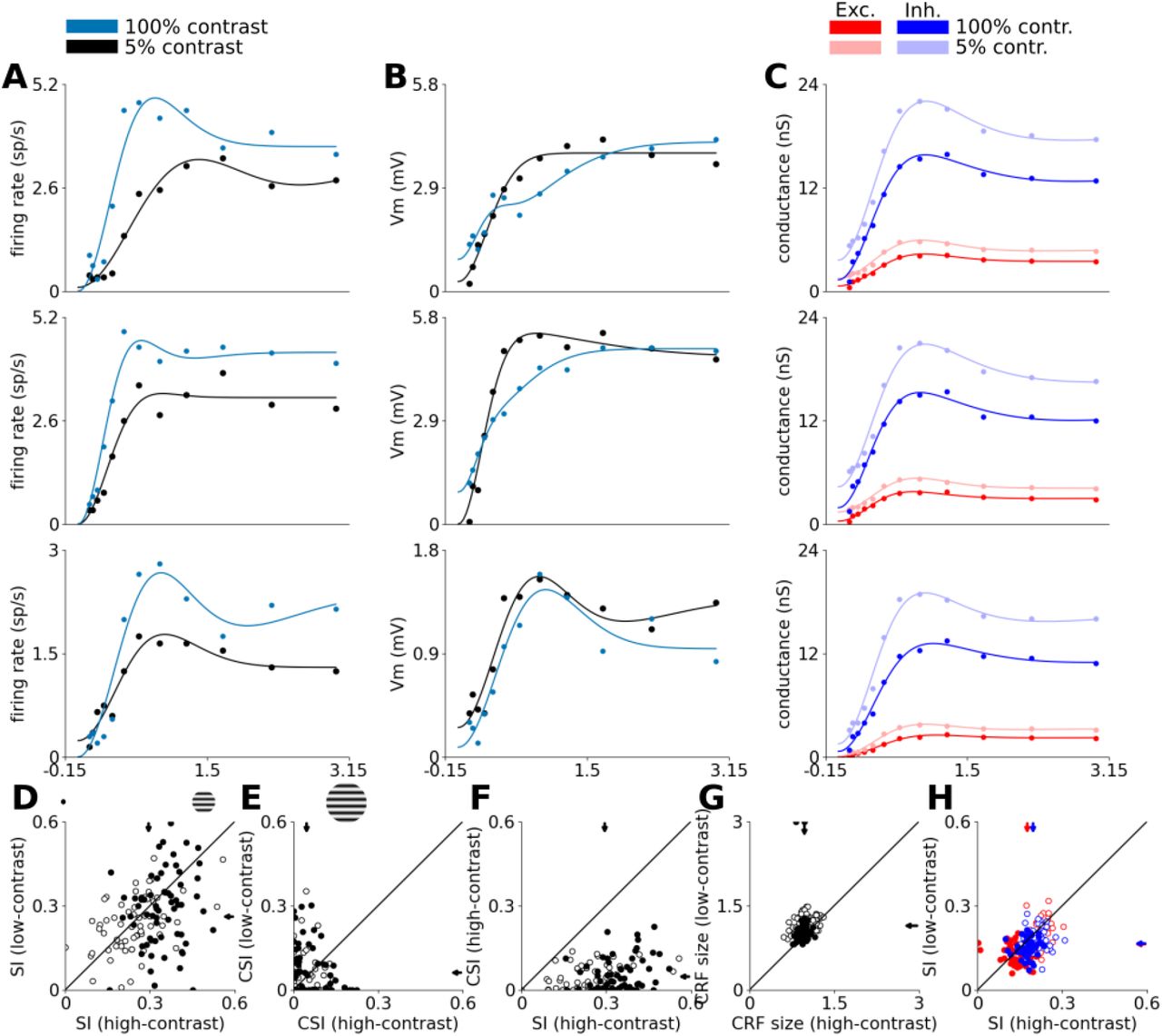