

Abstract
Despite considerable studies on the adaptation of plant pathogens to qualitative resistance, few theoretical studies have investigated whether and how quantitative resistance can select for increased pathogen aggressiveness. In this paper, we formulate an integro-differential model with nonlocal effects of mutations to describe the evolutionary epidemiology of fungal plant pathogens in heterogeneous agricultural environments. Parasites reproduce clonally and each strain is characterized by several pathogenicity traits corresponding to the basic infection steps (infection efficiency, latent period, sporulation capacity depending on the age of infection). We first derive a general expression of the basic reproduction number ℛ0 for fungal pathogens in heterogeneous host environments, typically several cultivars cultivated in the same field (cultivar mixtures) or in different fields landscape (mosaics). Next, by characterizing the evolutionary attractors of the coupled epidemiological evolutionary dynamics, we investigate how the choice of quantitative resistances altering different pathogenicity traits impact the evolutionary dynamics of the pathogen population both at equilibrium and during transient epidemiological dynamics. We show that the model admits an optimization principle relying on an ℛ0 maximization approach for traits involved in the infection cycle after spore germination. We also highlight that within-host correlation between such traits (typically between the latent period and total number of spores produced during the infectious period) impact resistance durability and, more generally, how one may take advantage of evolutionary dynamics to increase the durability of quantitative resistance. Our analyses can guide experimentations by providing testable hypotheses and help plant breeders to design breeding programs.
1 Introduction
Resistance to parasites, i.e. the capacity of a host to decrease its parasite development (Raberg et al., 2009; Restif & Koella, 2004), is a widespread defense mechanism in plants. Qualitative resistance usually confers disease immunity in such a way that parasites exhibit a discrete distribution of their disease phenotype (“cause disease” versus “do not cause disease”) (McDonald & Linde, 2002). Quantitative resistance leads to a reduction in disease severity (Poland et al., 2009; St. Clair, 2010) in such a way that parasites exhibit a continuous distribution of their quantitative pathogenicity (McDonald & Linde, 2002; St. Clair, 2010; Lannou, 2012). Quantitative pathogenicity, also termed aggressiveness, can be estimated in laboratory experiments through the measure of a small number of pathogenicity traits (Pariaud et al., 2009; Lannou, 2012) expressed during the basic steps of the host-pathogen interaction. Quantitative resistance genes alter their expression, sometimes through pleiotropic effects (i.e. effects on more than one trait (Parlevliet, 1986; Richardson et al., 2006)). Quantitative resistance has gained interest in plant breeding for pathogen control in low-input cropping systems, in particular due to their supposed higher durability compared to qualitative resistance (Mundt, 2014; Niks et al., 2015). However plant pathogens also adapt to quantitative resistance (see Pilet-Nayel et al. (2017) for a review). The resulting gradual “erosion” of resistance efficiency (McDonald & Linde, 2002) corresponds, from the pathogen side, to a gradual increase in quantitative pathogenicity.
Few theoretical studies have investigated how the deployement of quantitative resistance in agrosystems impact pathogen aggressiveness (Iacono et al., 2012; Bourget al., 2015; Rimbaud et al., 2018). These studies must address the fundamental short- and long-term objectives of sustainable management of plant diseases (Zhan et al., 2015; Rimbaud et al., 2018): the short-term goal focuses on the reduction of disease incidence, whereas the longer-term objective is to reduce the rate of evolution of new pathotypes. The evolutionary epidemiology analysis are well-suited for this purpose (see e.g., Day & Proulx (2004); Day & Gandon (2006)). Essentially inspired by quantitative genetics, it accounts for the interplay between epidemiological and evolutionary dynamics on the same time scale. As such it can be used to monitor the simultaneous dynamics of epidemics and evolution of any set of pathogen life-history trait of interest. It can also handle heterogeneous host populations resulting, for example, from differences in their genetic composition (Gandon & Day, 2007). This is typically the case of field mixtures, where several cultivars are cultivated in the same field, and of landscapes mosaics, with cultivars cultivated in different fields.
In this article, we follow this approach and study the evolutionary epidemiology of spore-producing pathogens in heterogeneous agricultural environments. Plant fungal pathogens (sensu lato, i.e. including Oomycetes) are typical spore-producing pathogens responsible for nearly one third of emerging plant diseases (Anderson et al., 2004). Here we use an integro-differential model where the pathogen traits are represented as a function of a N-dimensional phenotype. This model extends previous results of Djidjou-Demasse et al. (2017) to heterogeneous plant populations mixing cultivars with different quantitative resistances. First, we investigate how the choice of quantitative resistances altering different pathogenicity traits impact the pathogen population structure at equilibrium. This question is addressed by characterizing the evolutionary attractors of the coupled epidemiological evolutionary dynamics. A particular emphasis will be put here on the differences between the cornerstone concepts of ℛ0 in epidemiology (Diekmann et al., 1990; van den Driessche & Watmough, 2008) and invasion fitness in evolution. Secondly we investigate how this choice also impacts the transient behavior of the coupled epidemiological evolutionary dynamics.
2 A structured model of epidemiological and evolutionary dynamics
2.1 Host and pathogen populations
We consider an heterogeneous host population with Nc ≥ 2 host classes infected by a polymorphic spore-producing pathogen population. Here, host heterogeneity may refer to different host classes, typically plant cultivars, but more generally it can handle different host developmental stages, sexes, or habitats. The host population is further subdivided into two compartments: susceptible or healthy host tissue (S) and infectious tissue (I). In keeping with the biology of fungal pathogens, we do not track individual plants, but rather leaf area densities (leaf surface area per m2). The leaf surface is viewed as a set of individual patches corresponding to a restricted host surface area that can be colonized by a single pathogen individual. Thus only indirect competition between pathogen strains for a shared resource is considered. Spores produced by all infectious tissues are assumed to mix uniformly in the air and then land on any host class according to the law of mass action, that is the probability of contact between a spore and host k is proportional to the total susceptible leaf surface area of this host. The density of airborne spores is denoted by A.
The parasite is assumed to reproduce clonally. Its population is made of a set of genetic variant termed thereafter strains. At each infection cycle (i.e. generation), mutations randomly displace strains into this phenotype space. Each strain with phenotype x is characterised, on each host class, by pathogenicity traits that describe the basic steps of the disease infection cycle : (i) infection efficiency βk(x), i.e. probability that a spore deposited on a receptive host surface produces a lesion, (ii) latent period τk(x) and (iii) shape of the sporulation curve. In line with the biology of plant fungi (van den Bosch et al., 1988; Sache et al., 1997; Kolnaar & Bosch, 2011; Segarra et al., 2001), a gamma sporulation curve defined by three parameters is assumed : (i) total number of spores produced pk(x) during the infectious period, (ii) number of repeated sporulation events occurring on an individual foliar lesion nk(x) and (iii) rate of sporulation events λk(x). Parameters nk and λk defined the time shape of the sporulation curve (Figure 1A) by distributing the total amount of spores produced by a lesion (pk) over its average infectious period (nk/λk). Previous hypothesis lead to the following sporulation function :


A Two gamma sporulation curves rk(a, x) with latent period τk = 4 and total spore production pk = 80. B Spores production capacity (pk/pk,max) as a function of latency time (τk). The trade-off between the total number of spores produced (pk) and the probability for an infected tissue to survive the latent period (sk) is described by a power function. Its concavity is parametrized by α.
2.2 The model
We introduce a set of integro-differential equations modeling the epidemiological and the evolutionary dynamics of the host and pathogen populations just described. The general formulation used encompasses several simpler models of the litterature (Appendix B). A key feature of the model is to explicitly track both the age of infection and the pathogen strain. This leads to a non-local age-structured system of equations posed for time t > 0, age since infection a > 0 and phenotype x ∈ ℝN,

Table 1 lists the state variables and parameters of the model. Sk(t) is the density of healthy tissue in host k at time t, ik(t, a, x) the density of tissue in host k that was infected at time t − a by a pathogen with phenotype x, and A(t, x) denotes the density of spores with phenotype x at time t. Without disease, susceptible hosts are produced at rate Λ > 0 and die at rate θ > 0, regardless of their class. ϕk is the proportion of the host k at the disease-free equilibrium in the environment. With disease, susceptible hosts can become infected by air-borne spores. The total force of infection on a host k is hk(t) = ∫ βk(y)A(t, y)dy. Infected hosts die at rate θ + dk(a, x) where dk(a, x) is the disease-induced mortality of infected tissue. Airborne spores produced by infected hosts become unviable at rate δ > 0. Hosts infected by strain y produce airborne spores with phenotype x at a rate mε(x − y)rk(a, y), where mε(x − y) is the probability of mutation from phenotype y to phenotype x and rk(a, y) is the sporulation function, which depends on host class, age of infection and parasite phenotype.
Main notations, state variables and parameters of the model.
The kernel mε represents the effects of mutations that randomly displace phenotypes at each generation. It depends on a small parameter ε > 0 representing the mutation variance in the phenotypic space. To fix ideas, a multivariate Gaussian distribution m = N (0, Σ) leads to  . The covariance terms of Σ can allow to take into account correlations between pathogen life-history traits (Martin & Lenormand, 2006; Gandon, 2004). The mutation kernel m is not restricted to Gaussian distributions, provided it satisfies some properties such as positivity and symmetry (Appendix A).
Further, a correlation between the time-lag to maturity and fecundity has been sometimes observed for plant fungi (Pariaud et al., 2013). Here, the time-lag to maturity is measured by the probability for an infected host to survive the latent period  , and fecundity by the total number of spores produced pk(x). This relationship describes a phenotypic trade-off because short latent period and high sporulation capacity represent fitness advantages. The model can handle such a trade-off using a power function
  defined for z ∈ (0, 1) and parametrized by α > 0 which determines its global concavity (Egas et al., 2004; Débarre & Gandon, 2010). The within-host trade-off then writes (Figure 1B)
 where pk,max is the maximum of pk.
3 Fitness function and evolutionary attractors
3.1 The fitness function
The basic reproduction number, usually denoted ℛ0, is defined as the total number of infections arising from one newly infected individual introduced into a healthy (disease-free) host population (Diekmann et al., 1990; Anderson, 1991). The disease-free equilibrium density of susceptible hosts in class k is  . In an environment with Nc host classes, a pathogen with phenotype x will spread if ℛ0(x) > 1, with
 where the quantity
  , is the basic reproduction number of a pathogen with phenotype x in the host k, and the fitness function Ψk is given by
 for all k ∈ {1, …, Nc}. The quantity Ψk(x) is the absolute fitness, or reproductive value, of a pathogen with phenotype x landing on host k (see Appendix C for details on calculations).
Assuming that dk does not depend on the age of infection and a gamma sporulation function, we obtain the simpler expression

The above equation means that, (i) during its life time 1/δ, (ii) a propagule infects a leaf area at rate βk, (iii) this infected area survives the latent period with probability  , (iv) achieves nk sporulation events with probability λk/(λk + θ + dk) for each event and (v) produces a total number of spores pk during the infection period. Equation (3.6) can also handle within-host trade-offs where terms (iii) and (v) are linked by (2.3).
Finally, if furthermore rk is a constant (i.e. rk(a, x) = pk(x) and dk(a, x) = dk(x) for all a), we recover the classical expression of ℛ0 for SIR models, with  (Day, 2002).
3.2 Evolutionary Attractors
ℛ0 can be used to study the spread of a pathogen strain x in an uninfected host population. To study the spread of a new mutant strain in a host population already infected by a resident strain x, and to characterize pathogen’s evolutionary attractors among a large number of pathogen strains, we can use the adaptive dynamics methodology and calculate invasion fitness (Dieckmann, 2002; Diekmann et al., 2005; Geritz et al., 1997; Metz et al., 1996).
Invasion fitness
Here, we work in generation time and use the lifetime reproductive success of a rare mutant as a fitness proxy. Once the pathogen with phenotype x spreads, let us assume that the population reaches a monomorphic endemic equilibrium denoted by  . Note that Ex is the environmental feedback of the resident x. Calculations are detailed in Appendix C along with the expression of
  and Ax.
A rare mutant with phenotype y will invade the resident population infected by the strain x if the invasion fitness fx(y) of y in the environment generated by x is such that
 where
where

Quantities ℛ(y, Ex) and ℛ0(y), given by equations (3.4) and (3.7), have a strong analogy. Both expressions are basic reproduction numbers that measure the weighted contribution of the pathogen to the subsequent generations, but while ℛ0(y) is calculated in the disease-free environment  , ℛ(y, Ex) is calculated in the environment set Ex by the resident strain x.
Noteworthy ℛ(y, Ex) takes the form of a sum of the mutant pathogen’s reproductive success in each host class as between-class transmission can be written as the product of host susceptibility times pathogen transmissibility. This is equivalent to the more general statement that pathogen propagules all pass through a common pool, as in our model in the compartment A (Rueffler & Metz (2013)). However, this property is not generally true as showed by Gandon (2004) in a two-class model.
ℛ0 as proxy of invasion fitness
In general, finding the evolutionary attractors of host-pathogen systems is mostly based on properties of the invasion fitness on an adaptive landscape (Diekmann et al., 2005; Geritz et al., 1997, 1998; Nowak & Sigmund, 2004). A Pairwise Invasibility Plot (PIP) must then be used to characterize evolutionary attractors. However, when infection efficiencies do not differ between host classes (i.e. βk = β, ∀k), model (2.2) admits an optimisation principle (Mylius & Diekmann, 1995; Metz et al., 2008; Lion & Metz, 2018; Metz & Geritz, 2016; Gyllenberg & Service, 2011). More precisely, the evolutionary attractors of the model coincide with the maxima of the ℛ0. We prove in Appendix E that the invasion fitness fx(y) of a rare mutant with y-phenotype in the resident x-population is such that sign(fx(y)) = sign (ℛ0(y) − ℛ0(x)). We emphasise again that this is not a general property of host-pathogen systems (see e.g. Lion & Metz (2018) for a more general discussion)
4 Differential effect of pathogenicity traits targeted by resistance genes on the evolutionary dynamics of fungal disease
In this section, we firstly characterize the evolutionary attractors of the coupled epidemiological and evolutionary dynamics described by model (2.2) by analysing the shape of the ℛ0. Then, using simulations, we study how the population reaches this equilibrium state through a mutation-selection process and highlight how these transient dynamics may inform the sustainable management of resistance genes.
4.1 Case study : deployment of a plant resistant cultivar
We consider a monomorphic pathogen population resulting from the monoculture of a single plant cultivar, called susceptible (S), during a long-time. The S cultivar is infected by a pathogen density A0 with Gaussian distributed phenotypes which is well adapted on the S cultivar. At t = 0, a fraction φ ∈ (0, 1) of the S cultivar is replaced by a new cultivar bearing a quantitative resistance gene, called resistant cultivar (R). The resistance gene alters a single pathogenicity trait, characterized in both cultivars by normally distributed values with means −μ and μ on S and R cultivars, respectively. The inverse of their variance,  , define the selectivity of the S and R cultivars, respectively. Altogether, the parameters
  and
and  define the strength of the resistance gene efficiency by measuring to what extent the adaptation to one cultivar causes maladaptation to the other.
Two scenarios were considered: the resistance can either impose to the pathogen a trade-off on its total spore production (TSP scenario) or on its infection efficiency (TIE scenario). For each scenario, we illustrate how contrasted values of μ (a proxy of resistance efficiency) and φ (defining the deployment strategy) affect the evolutionary dynamics of the pathogen and the durability of the R cultivar. The durability was quantified by the time Tinf when at least 5% of the leaf area density of the R cultivar is infected (i.e. time t from which ∫IR(t, x)dx/ SR(t) + ∫ IR(t, x)dx is always ≥ 5%) (Rimbaud et al., 2018). In practice this is the time where the erosion of the R gene become detectable in the field. All model parameters and initial conditions used for the simulations are summarized in Table 2.
Initial conditions and parameters used for the simulations with two host classes (S and R cultivars). Two scenarios were considered: the R cultivar can either alter the Infection Efficiency of the pathogen (TIE) or its total Spore Production (TSP). 𝒩 stands for the density function of the normal distribution.
4.2 Evolutionary dynamics with resistance genes impacting sporulation
When the R gene impacts the total spore production of the pathogen, the maximum points of the ℛ0 are given by  and
and  (Figure 2 A, Appendix F). The ℛ0 optimization principle holds here, and the population always becomes monomorphic around an evolutionary attractor characterized by the maximum of ℛ0 (Section 3.2). We show how μ (a proxy of resistance efficiency) and φ (proportion of the R cultivar deployed) impact the shape of ℛ0 (number of modes and their steepness) and the transient dynamics (Figure 3).
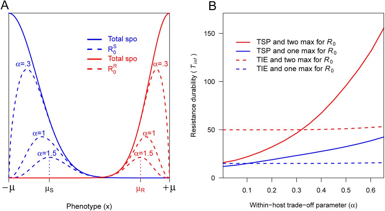
A Characterization of phenotypes μS and μR maximizing the ℛ0 on S and R cultivars. The phenotypes with maximal spore production are located at −μ and +μ for the S and R cultivars respectively. But these are not the phenotypes with the maximal basic reproduction numbers  which are located at μk due to the within-host trade-off, parametrized by α, between spores production pk and the probability for an infected host to survive the latent period sk (with k ∈ {S, R}). B Impact of the within-host trade-off parameter (α) on the durability of the resistant cultivar (Tinf). Other parameters are the same as for Figures 3 and 4.

Evolutionary epidemiology dynamics when the resistance impacts the total spore production of the pathogen pk for three configurations of the fitness function Ψ and with a within-host trade-off parameter α = 0.2. A-C The fitness function is unimodal: μ = 0.055; μS ≃ −0.023; μR ≃ 0.023. At t = 0, the pathogen population, essentially concentrated around the phenotype μS, is adapted on the S cultivar. The dynamics of the density of infected tissue and the phenotypic composition of the pathogen population in the S and R cultivars are display in B and C respectively, with Tinf = 19. Panels D-F and G-I are organized similarly with Tinf = 32 and 28 respectively. D-F and G-I The fitness function is bimodal with a unique global maximum μR (μ = 0.1; μS ≃ −0.07, μR ≃ 0.07) but a local maximum also exists around μS. The value of φ = 0.55 in panels G-I implied that μS is closer to μR compared to panels D-F where φ = 0.51. In panels C,F,I the dash-blue line represents Tinf.
With a unique maximum of ℛ0
This maximum point, located at μ∗(μS < μ∗ < μR), is the unique evolutionary attractor (Figure 3 A) which corresponds to a generalist pathogen. The fast transient dynamics observed on simulations, with a pathogen population rapidly concentrating around μ∗ (Figure 3 B,C), corresponds to a fast erosion of the quantitative R (Figure 3 C).
With two local maxima of ℛ0
ℛ0 is maximized (globally) by a single phenotype around μR but a local maximum also exists around μS (Figure 3 D). The ℛ0 maximization principle indicates that μR is the evolutionary attractor at equilibrium. This phenotype is a specialist of the R cultivar. The pathogen population lives for a relatively long time around the initially dominant phenotype μS and then shifts by mutation on μR (Figure 3 E,F). These dynamics occur simultaneously on the S and R cultivars. The durability of the R cultivar (as measured by Tinf) can be relatively long if the R cultivar remained firstly dimly (and decreasingly) infected. The choice of the proportion of R cultivar sown in the landscape is important for durability. Values of φ bringing closer the fitness peaks (in the sense ℛ0(μS) ⪅ ℛ0(μR)) will lower the durability Tinf even if the shift toward the evolutionary attractor takes a longer time (Figure 3 G-I).
4.3 Evolutionary dynamics with resistance genes impacting infection efficiency
When the R gene impacts the infection efficiency of the pathogen, the within-host trade-off does not impact maximums points of the ℛ0. We have μS = −μ and μR = μ (Appendix F). As the optimization principle does not hold, the shape of ℛ0 function does not allow to characterize evolutionary attractors. PIP must be used instead (see Figure S1 for an illustration). In sharp contrast with the TSP scenario, two configurations - corresponding to monomorphic or dimorphic populations - are possible.

Here we have a polymorphic pathogen population at equilibrium in different proportions (panels d,e) but only one local maximum for the ℛ 0 as confirmed by the gradient (panels b,c). However, the PIP predicts a polymorphic population (panel a). Indeed, singular strategies, μS and μR, are respectively branching point and evolutionarily stable (no nearby mutant can invade). Here, we have fixed φ = 0.64, σS = 0.06, σR = 0.04 and μS = −μR = −0.0579.
In the first configuration, the pathogen population is composed of a single generalist at equilibrium (Figure 4 A-C). In the second configuration, the pathogen population is composed of two evolutionary attractors corresponding to specialists of each cultivars (Figure 4 panels D-F). Formally, dimorphism occurs if there exists two constants aS, aR > 0 defined by system (D.15), and typically quantifying weights of each strain μS and μR at the equilibrium (Appendix D). In practise, with a R gene targeting infection efficiency, each cultivar is infected by a specific strain. At equilibrium, the pathogen population is composed of different proportions of the two evolutionary attractors μS and μR (Figure 4 E-F). This is not the case for a R gene targeting sporulation wherethe S and R cultivars are simultaneously infected at a given time by the same pathogen strain (Figure 3 D-I).

Evolutionary epidemiology dynamics when the resistance impacts the pathogen infection efficiency βk for three configurations of the fitness function Ψ and with a within-host trade-off parameter α = 0.2. A-C A unique evolutionary attractor μ∗ for the PIP (sign of the invasion fitness fz(y)): μ = 0.055; μS = −0.0552; μR = 0.0552. At t = 0, the pathogen population, essentially concentrated around the phenotype μS, is adapted on the S cultivar. The dynamics of the density of infected tissue and the phenotypic composition of the pathogen population in the S and R cultivars are displayed in B and C respectively, with Tinf = 17. Panels D-F is organized similarly with Tinf = 50 and 44 respectively. D-F Two evolutionary attractors μS and μR for the PIP: μ = 0.1; μS ≃ −0.0989; μR ≃ 0.0989. In panels C,F the dash-blue line represents Tinf. Here, singular strategies μ∗, μS and μR are evolutionarily stable (no nearby mutant can invade): in the PIP, the vertical line through μ∗ (panel A), μS or μR (panels D) lies completely inside a region marked ‘−’.
5 Discussion
This work follows an ongoing trend aiming to jointly model the epidemiological and evolutionary dynamics of host-parasite interactions. Our theoretical framework, motivated by fungal infections in plants, allows us to tackle the question of the durability of plant quantitative resistance genes altering specific pathogen life-history traits. Many problems and questions are reminiscent of the literature on the epidemiological and evolutionary consequences of vaccination strategies. For instance, quantitative resistance traits against pathogen infection rate, latent period and sporulation rate are analogous to partially effective (imperfect) vaccines with anti-infection, anti-growth or anti-transmission modes of action, respectively (Gandon et al., 2001). Similarly, the proportion of fields where a R cultivar is deployed is analogous to the vaccination coverage in the population (Gandon & Day, 2007).
Evolutionary outcomes with multimodal fitness functions
In line with early motivations for developing a theory in evolutionary epidemiology (Day & Proulx, 2004), we investigated both the short- and long-term epidemiological and evolutionary dynamics of the host-pathogen interaction. Although the short-term dynamics is investigated numerically, the long-term analysis is analytically tractable and allows us to predict the evolutionary outcome of pathogen evolution. In contrast with most studies in evolutionary epidemiology, the analysis proposed allows us to consider multimodal fitness functions, and to characterize evolutionary attractors at equilibrium through a detailed description of their shape (number of modes, steepness and any higher moments with even order). Similarly, our results are neither restricted to Gaussian mutation kernel m (see also Mirrahimi (2017)), provided that m is symmetric and positive (Appendix A), nor to rare mutations as in the classical adaptive dynamics approach.
In our work, the TSP model admits an optimisation principle and potential evolutionary attractors are located at the peaks ℛ0. This is not always the case for the TIE model (except for some special configurations). An important consequence of the existence of an optimisation principle is that evolutionary branching (i.e. a situation leading to pathogen diversification and to long term coexistence of different pathogen strategies) is impossible.
ℛ0 expression for fungal pathogens in heterogeneous host environment
Usually, the computation of ℛ0 is based on the spectral radius of the next generation operator (NGO) (Diekmann et al., 1990; Diekmann & Heesterbeek, 2000). The method was applied by van den Bosch et al. (2008) to calculate the ℛ0 for lesion forming foliar pathogens in a setting with only two cultivars and no effect of the age of infection a on sporulation rate and disease-induced mortality. Here, we follow the methodology based on the generation evolution operator (Inaba, 2012) to derive an expression for the basic reproduction number ℛ0 in heterogeneous host populations composed of Nc cultivars (Appendix C).
Lannou (2012) pointed out the need for ℛ0(x) expressions allowing to compare the fitness of competing pathogen strains with different latent periods. We provide such an expression of ℛ0 (3.4) for the classical gamma sporulation curve proposed by Segarra et al. (2001) and observed for several plant fungi (van den Bosch et al., 1988; Sache et al., 1997; Kolnaar & Bosch, 2011; van den Bosch et al., 1988). This expression combine (i) the pathogenicity traits expressed at the scale of the plant during the basic infection steps (infection efficiency βk(x), latent period τk(x) and shape of the sporulation function pk(x), nk(x) and λk(x)) with (ii) the proportion of each cultivar k in the environment (φk). As these traits can be measured in the laboratory, ℛ0(x) bridges the gap between plant-scale and epidemiological studies, and between experimental and theoretical approaches. ℛ0-based approach have been for example used to compare the fitness of a collection of isolates of potato light blight (Montarry et al., 2010), to highlight the competition exclusion principle for multi-strains within-host malaria infections (Djidjou-Demasse & Ducrot, 2013) and to predict the community field structure of Lyme disease pathogen from laboratory measures of the three transmission traits (Durand et al., 2017).
ℛ0 as a proxy of invasion fitness for pathogenicity traits involved in infection cycle after spore germination
In the context of model (2.2), the function Ψ(x), which is proportional to ℛ0(x), is an exact fitness proxy for competing strains differing potentially for the latent period and/or the shape of the sporulation function. The basic reproduction number ℛ0 can thus be used to investigate how basic choices made when deploying a new resistance (resistance gene choice, proportion cultivated) impact resistance durability and the emergence of specialist or generalist pathogen. With a unique local maximum of ℛ0, a generalist pathogen will selected while with two local maxima a specialist is selected. But, in any case, the pathogen population will become monomorphic at equilibrium after the deployment of a R cultivar impacting any pathogenicity traits expressed after spore germination (e.g. TSP scenario) as the optimization principle avoid evolutionary branching. However, more generally, a clear distinction between pathogen invasion fitness ℛ(x, y) and epidemiological ℛ0(x) is necessary to properly discuss the adaptive evolution of pathogens (Lion & Metz, 2018). In our case study, the deployment of a R cultivar impacting infection efficiency (TIE scenario) can lead to the selection of either a monomorphic population with a generalist pathogen or a polymorphic population with two specialist pathogens (Figure 4). The occurrence of such evolutionary branching is of practical importance for management purposes as evidenced for example in the wheat rust fungal disease where disease prevalence varies with the frequencies of specialist genotypes in the rust population (Papaïx et al., 2011).
Our results also highlight that a detailed knowledge of within-host pathogenicity trait correlations is required to manage resistance durability. Only few studies taking explicitly into account evolutionary principles compared how resistant cultivars targeting different aggressiveness components of fungal pathogens impact durability (Iacono et al., 2012; Bourget al., 2015; Rimbaud et al., 2018). These studies assumed that aggressiveness components are mutually independent while correlations have been sometimes identified between latent period and propagule production (Pariaud et al., 2009; Lannou, 2012; Nidelet et al., 2009; Pariaud et al., 2013). We show that such correlations impact durability when quantitative resistance targets any traits involved in the infection cycle after spores germination on a receptive host leaf. In the TSP scenario, Tinf can increase substantially with the within-host trade-off parameter α (Figure 2 B), as a result of the term involving α in the equations of the maximum points μS and μR of the ℛ0. Therefore, any guidelines aiming to help plant breeders to adequately choose resistance QTLs in breeding programs should consider these potential correlations, in particular for quantitative R gene targeting any traits involved in the infection cycle after spore germination on a receptive host leaf.
Notes on some model assumptions
The model assumes an infinitely large pathogen population. Demographic stochasticity is thus ignored while it can impact evolutionary dynamics (e.g., lower probabilities of emergence and fixation of beneficial mutations, reduction of standing genetic variation (Kimura, 1962)). In particular, genetic drift is more likely to impact the maintenance of a neutral polymorphism rather than of a protected polymorphism where selection favors coexistence of different genotypes against invasions by mutant strategies (Geritz et al., 1998). The effect of genetic drift depends on the stability properties of the model considered. As our model has a unique globally stable equilibrium, genetic drift is likely to play a much lesser role than with models characterized by unstable equilibrium. Moreover large Ne in the range ≃ 103 - 3.104 have been reported at field scale for several species of wind-dispersed, spore-producing plant pathogens (Ali et al., 2016; Zhan et al., 2001; Walker et al., 2017), suggesting a weak effect of genetic drift for their evolution.
The model assumes a unique pool of propagules and spore dispersal disregard the location of healthy and infected hosts. This assumption is more likely when the extent of the field or landscape considered is not too large with respect to the dispersal function of airborne propagules. Airborne fungal spores often disperse over substantial distances with mean dispersal distance in the range 102 to 103 meters and, in most case, fat-tail dispersal kernels associated to substantial long-distance dispersal events (Fabre et al. (2020) for a review). Recently Mirrahimi (2017) used integro-differential equations to describe a phenotypically structured population subject to mutation, selection and migration between two habitats. Rimbaud et al. (2018) used a stochastic spatially-explicit model to assess the epidemiological and evolutionnary outcomes of resistant deployement. It would be interesting to draw on these examples and extend our approach to a spatially explicit environment. When dispersal decreases with distance, large homogeneous habitats promote diversification while smaller habitats, favoring migration between distinct patches, hamper diversification (Débarre & Gandon, 2010; Haller et al., 2013; Papaïx et al., 2013). Managing the resulting population polymorphisms, either for conservation purpose in order to preserve the adpative potential of endangered species or for disease control purpose in order to hamper pest and pathogen adaptation should become a priority (Vale, 2013).
Code availability
The MATLAB codes used to simulate the model and generate the figures have been deposited in Dataverse at https://doi.org/10.15454/WAEIMA
A Properties of the mutation kernel mε
The kernel function mε arising in model (2.2) should satisfy the following properties:
(H1) The function mε is almost everywhere strictly positive on ℝN and should be normalised such that,

This last condition expresses that all interactions generated on the phenotypic space of pathogens necessarily end up somewhere on that space.
(H2) Its variation should only depend on the distance separating the points between which the interactions are evaluated (i.e. mε(x) = mε(−x), for all x ∈ ℝN).
(H3) It is highly concentrated and decays rather fast at infinity in the sens that mε(x) = ε−N m(x/ε) and  .
.
B Some special cases of the general model (2.2)
By omitting the age structure, we re-write model (2.2) as follows
 wherein we take into account the (host and strain-specific) duration of the sporulation period, denoted by lk(x).
Furthermore, if we assume that there are no “interactions” in the phenotypic space of pathogens, i.e. without mutations: ε → 0, then the simplified model (B.1) rewrites

C The fitness function
In this appendix we explain how to compute the fitness function. To that aim, by formally taking the limit ε → 0 into (2.2), this system becomes

Let us assume that system (C.3) reaches a monomorphic epidemiological equilibrium  , for some trait z, before a new mutation with trait value, say, y occurs. Note that Ez is the environmental feedback of the resident z. We introduce a small perturbation in (C.3) in the phenotype trait y, so that the evolution of the system reads as follows:
  and
and
 and the small perturbations for the infection, jk and B, are governed by the linearized system of equations around Ez. This reads as

In order to study the evolution of this perturbation we will derive a renewal equation on bz(t, y), the density of newly produced spores at time t with phenotype y in the resident population with phenotype x. This term is more precisely defined by

It then follows from the jk-equation of the linear system (C.4), that
 while
while

As a consequence, bz(t, y) satisfies the following renewal equation:
 wherein we have set

Then (C.5) can be rewritten as
 where Bz(a, y) is the expected number of new infections produced per unit time, in a resident host population with phenotype z, by an individual which was infected a units of time ago with the phenotype y, given by

Due to the above formulation, it follows from classical adaptive dynamics (Diekmann et al., 2005; Geritz et al., 1997; Metz et al., 1996) that the spore numbers, ℛ(y, Ez), of a rare mutant strategy, y, in the resident z-population is given by
 wherein
  . Then, the invasion fitness fz(y) of a mutant strategy y in the resident z-population is given by

Note that when the environmental feedback Ez is reduced to the disease-free environment, then  re-writes as
  . And the epidemiological basic reproduction number of the pathogen with the phenotype y is calculated as

Once the pathogen has spread and reached the monomorphic equilibrium, then the endemic feedback environment Ez becomes
 where Az > 0 is the unique solution of the following equation (only defined when ℛ0(z) > 1):

D Dimorphic or monomorphic equilibrium
To simplify the presentation, we consider system (2.2) with Nc = 2 corresponding to S and R cultivars. Denote by (S0, i0(·), A0) the endemic equilibrium of system (2.2) as ε → 0 and when only S is cultivated (i.e. when the proportion φ of R is zero). From results in (Djidjou-Demasse et al., 2017) we have

Now, let (SS, SR, iS(·), iR(·), A) be an equilibrium of system (2.2) when a proportion φ > 0 of R is cultivated. Next recall that, for k ∈ {S, R},
 so that A(·) becomes a solution of the nonlinear equation:

Using this equation we heuristically explore conditions yielding to dimorphic or monomorphic equilibrium.
Resistant gene altering infection efficiencies βS and βR (TIE scenario)
We formally assume that the population of spores writes  , and we plug this ansatz into equation (D.10) above. This yields, for any x,

Letting ε → 0 and recalling that mε(x) ≈ δ0(x), one obtains
 that is

As a consequence, for the equilibrium to be dimorphic, namely aR > 0 and aS > 0, it is necessary that there exist aR > 0 and aS > 0 satisfying the following system of equations:

We set

Recall that with the TIE scenario we have rS = rR and dS = dR such that the fitness function  , takes the form Ψk = c0βk for k = S, R (where c0 is the same positive funtional for S and R). Doing that, the above system rewrites
 wherein
  and c0 = c0(μS) = c0(μR). With the TIE scenario (i.e. with trade-off on infection efficiency βk), we reasonably have βR(μR) > βR(μS) and βS(μS) > βS(μR). Therefore, det(𝒦) = φ(1 − φ) (βR(μR)βS(μS) − βR(μS)βS(μR)) > 0. Then, solving system (D.12) for (X, Y) yields to

Since  , the above system rewrites

Coming back to the definition of X = X(aS, aR) and Y = Y (aS, aR) provided by (D.11), we then find
 with
with  . Because det(𝒢) = (βS(μR) βS(μS) − βR(μS) βS(μR)) > 0, it comes that for the equilibrium to be dimorphic it is necessary that

This heuristic condition (D.14) is necessary (but not sufficient) for system (2.2) (here with Nc = 2) to admit an endemic dimorphic equilibrium. The situation with a technical assumption on disjoint supports of βk, is rigorously studied in Burie al. (2019).
But here, in order to go slightly further in our analysis, we assume a strong trade-off on infection efficiency, namely

We deduce that the above system of equation roughly simplifies into

Hence the proportions of each phenotype, μS and μR, can be calculated as
 provided the following threshold conditions in this strong trade-off framework

As a consequence, the density of healthy hosts at equilibrium, when a proportion φ > 0 of R is cultivated, writes

Therefore, (D.9)-(D.16) lead to SS + SR = (1/ΨS(μS) + 1/ΨR(μR)) > S0 = 1/ΨS(μS) meaning that with a strong-trade off on infection efficiency, the time during which a proportion φ > 0 of R gene deployed remains beneficial (in terms of Healthy Area Duration gain) can be considered as large as possible.
Resistant gene altering total sporulation production pS and pR (TSP scenario)
In this case, using the same argument as in (Djidjou-Demasse et al., 2017) we can prove that the spore population is monomorphic at equilibrium such that  ; with a∗ > 0, providing that we are not in a strict symmetric configuration of the fitness function. Moreover, with a strong trade-off on sporulation rate, it is well known that μ∗∈ {μS, μR}. Then, applying the same arguments as in the previous section lead to

Again with ε → 0, it comes
 with ℛ0(μ∗) > 1.
Therefore, the density of healthy hosts at equilibrium, when a proportion φ > 0 of R is cultivated, writes

Therefore, (D.9)-(D.17) lead to SS + SR > S0 if and only if Ψ(μ∗) < ΨS(μS) meaning that with a strong-trade off on infection efficiency: (i) if Ψ(μ∗) < ΨS(μS) the time during which a proportion φ > 0 of R gene deployed remains beneficial (in terms of Healthy Area Duration gain) can be consider larger as possible; (ii) else, this time is quantified by the unique time T such that SS(t) + SR(t) ≥ S0(t) for all 0 < t ≤ T.
E R0 as the fitness proxy
By Equations (C.6) and (C.7), it comes

Using Equation (C.8) defining the resident equilibrium, i.e. ℛ(z, Ez) = 1, (E.18) becomes

When infection efficiencies do not differ between host classes (i.e. βk = β(x), for every k and every x). Then (E.19) gives
 and then

F Maximum points of the fitness function
Here we explicitly determine maxima of the fitness function (3.6) which writes:

With the normally distributed function hypothesis, in the TSP scenario, the resistance imposes a trade-off on the total number of spores, such that
 and infection efficiencies βk,s are constants (i.e. βS(x) = βR(x) = β0), wherein p0, β0 are positive constants. Since dk = 0, (F.21) takes the form

We then find that Ψk’s maximum points are  and
and  for S and R respectively.
In the TIE scenario, the resistance imposes a trade-off on the infection efficiency, such that
 and the total spores produced pk, are constants (i.e. pS(x) = pR(x) = p0). Again, since dk = 0, (F.21) takes the form

We then find that the maximum points of Ψk are −μ and μ for S and R respectively. Here, the within-host trade-off does not impact the optimal phenotype of the fitness function.
Acknowledgements
Authors thank Loup Rimbaud for comments and suggestions on the manuscript.
References


