

Abstract
Abstract The interpretation of variants in cancer is frequently focused on direct protein coding alterations. However, this analysis strategy excludes somatic mutations in non-coding regions of the genome and even exonic mutations may have unidentified non-coding consequences. Here we present RegTools (www.regtools.org), a free, open-source software package designed to integrate analysis of somatic variant calls from genomic data with splice junctions extracted from transcriptomic data in order to efficiently identify variants that may cause aberrant splicing in tumors.
Contributions Y.-Y.F. was involved in all aspects of this study, including designing methodology, developing and testing the tool software, analyzing and interpreting data, and writing the manuscript, with input from A.R., K.C.C, Z.L.S., J.K., D.F.C., O.L.G., and M.G. A.R. designed the tool and led software development efforts. Y.L., W.C.C., R.U., and R.G. provided unpublished tumor datasets and provided critical feedback on the manuscript. O.G. and M.G. supervised the study. All authors read and approved the final manuscript
Alternative splicing of messenger RNA is a biological process which allows a single gene to encode multiple gene products, increasing a cell’s functional diversity and regulatory precision. However, splicing malfunction can lead to imbalances in transcriptional output or even the presence of oncogenic novel transcripts1. The interpretation of variants in cancer is frequently focused on direct protein coding alterations2. However, most somatic mutations arise in intronic and intergenic regions, and exonic mutations may also have unidentified consequences. For example, mutations can affect splicing either in trans, by acting on splicing effectors, or in cis, by altering the splicing signals located on the transcripts themselves3. Increasingly, we are beginning to see the importance of splice variants in disease processes, not least of which in cancer. However, our understanding of the landscape of these variants is limited and few tools exist for their discovery. Few tools are directed at linking aberrant splicing to variants in cis and most are tailored to a narrow set of scientific aims4,5,6. Here we present RegTools, a free, opensource (MIT license) software package designed to efficiently identify potential cis-acting splice-relevant variants in tumors (www.regtools.org).
RegTools is a suite of tools designed to aid users in a broad range of splicing-related analyses. At the highest level, it contains three sub-modules: a variants module to annotate variant calls, a junctions module to analyze aligned RNAseq data and associated splicing events, and a cis-splice-effects module that combines these submodules, integrating genomic variant calls and transcriptomic sequencing data to identify potential splice-altering variants. Each sub-module contains one or more commands, which can be used individually or integrated into regulatory variant analysis pipelines.
The variants annotate command takes a VCF containing somatic variant calls and a GTF of transcriptome annotations as input. RegTools does not have any particular preference for variant callers or reference annotations. Each variant is annotated with known overlapping genes and transcripts and its putative splicing relevance based on position relative to known exons, which we call the “variant type”. The variant type annotation depends on the stringency for splicing-relevance the user sets through the “splicing window” setting. By default, RegTools marks intronic variants within 2 bp from the exon edge as “splicing intronic”, exonic variants within 3 bp as “splicing exonic”, other intronic variants simply as “intronic”, and other exonic variants simply as “exonic” and considers only “splicing intronic” and splicing exonic” as important. To allow for discovery of an arbitrarily expansive set of variants, RegTools allows the user to customize the size of the exonic/intronic windows individually (e.g. -i 20 -e 5 for intronic variants 20 bp from an exon edge and exonic variants 5 bp from an exon edge) or consider all exonic/intronic variants as potentially splicing-relevant (e.g. -E or -I) (Fig. la).

a, By default, variants annotate marks variants within 3bp on the exonic side and 2bp on the intronic side of an exon edge as potentially splicing-relevant. This “splicing window” can be modified individually for the exonic side and intronic side using the “-e” and “-i” options, respectively. With cis-splice-effects identify, for each variant in the splicing window, a variant region is determined by finding the largest span of sequence space between exons which flank the exon associated with the splicing-relevant variant. The variant region can also be set manually to contain the entire sequence space n bases upstream and downstream of the variant using the “-w” option. Junctions overlapping the variant region are associated with the variant. Using the -E option considers all exonic variants as potentially splicing-relevant, but is otherwise the same. The -I option considers all intronic variants and also limits the variant region to the intronic region in which the variant is found, excluding the flanking exons. b, Cis-splice-effects identify and the underlying junctions annotate command annotate splicing events based on whether the donor and acceptor site combination are found in the reference transcriptome GTF. In this example, there are two transcripts (shown in blue) which overlap a set of junctions from RNAseq data (depicted as junction supporting reads in red). Comparing the observed junctions to the reference junctions in the first transcript (top panel), RegTools checks to see if the observed donor and acceptor splice sites are found in any of the reference exons and also counts the number of exons, acceptors, and donors skipped by a particular junction. Double arrows represent matches between observed and reference acceptor/donor sites while single arrows show novel splice sites. These steps are repeated for the rest of the relevant transcripts, keeping track of whether there are known acceptor-donor combinations. Junctions with a known acceptor but novel donor or vice-versa are annotated as “A” or “D”, respectively. If both sites are known but do not appear in combination in any transcripts, the junction is annotated as “NDA”, whereas if both sites are unknown, the junction is annotated as “N”. If the junction is known to the reference GTF, it is marked as “DA”. c, The cis-splice-effects identify command relies on the variants annotate, junctions extract, and junctions annotate submodules. This pipeline takes variant calls and RNA-seq alignments along with genome and transcriptome references and outputs information about novel junctions and associated potential cis splice-altering sequence variants. RegTools is agnostic to downstream research goals and its output can be filtered through user-specific methods and thus can be applied to a broad set of scientific questions.

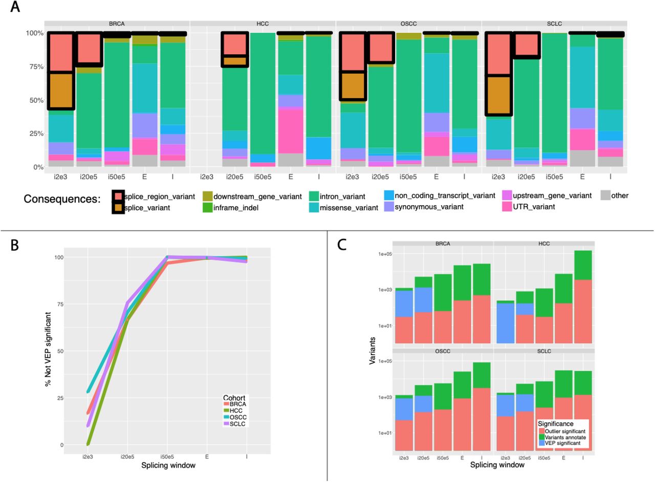
a, Variants determined as significant based on the outlier method were annotated using VEP with the “pick” and “per_gene” options. Only “pick” results were shown here, though both modes produced similar results. Stacked bars represent the percentage of total VEP annotations for each splicing window size across all variants discovered in each cohort. Blocks showing splicing-relevant annotations are highlighted with a black border. Annotation consequences are based on VEP consequences but similar annotations have been consolidated for clarity ({3_prime_UTR_variant, 5_prime_UTR_variant} → UTR_variant; {inframe_insertion, inframe_deletion} → inframe_indel; {splice_donor_variant, splice_acceptor_variant} → splice_variant; {mature_miRNA_variant, coding_sequence_variant, frameshift_variant, intergenic_variant, NMD_transcript_variant, non_coding_transcript_exon_variant, regulatory_region_variant, start_lost, start_gained, stop_lost, stop_gained, TF_binding_site_variant, protein_altering_variant} → other). b, Initially, in the default splicing window size, only a small portion of variants identified using the outlier method are not annotated as splicing relevant by VEP. However, as we extend the scope of our discovery, VEP quickly begins to miss potentially important splicing-relevant variants. c, Variant counts are displayed in overlaying bars (values scaled by log10). Cis-splice effects identify produces a large number of ostensibly false positive calls which must be narrowed down by downstream filtering methods. Using VEP as a downstream filter is not particularly helpful as it over-calls in the smaller splicing windows (i2e3 and i20e5) and under-calls in the larger ones. The outlier method provides a more consistent level of filtering which simplifies downstream analysis.
The junctions module contains the extract and annotate commands. The extract command takes a BAM file containing aligned RNAseq reads, infers the exon-exon boundaries based on the CIGAR strings7, and outputs each “junction” as a feature in BED12 format. The annotate command takes a file of junctions in BED12 format, such as the one output by junctions extract, a FASTA file containing the reference genome, and a GTF file containing reference transcriptome annotations and generates a TSV file, annotating each junction with: the number of acceptor sites, donor sites, and exons skipped and known overlapping transcripts and genes. We also annotate the “junction type”, which denotes if and how the junction is novel (i.e. discrepant compared to known transcript annotations). If the donor is known but the acceptor is not or vice-versa, it is marked as “D” or “A”, respectively. If both are known but the pairing is not known, it is marked as “NDA”, whereas if both are unknown, it is marked as “N”. If the junction is not novel (i.e. it appears in one or more transcripts of the supplied GTF), it is marked as “DA” (Fig. lb).
The cis-splice-effects module contains the identify command which identifies potential splice-altering variants from tumor sequencing data. The following are required as input: a VCF file containing variant calls, a BAM file containing aligned RNA-sequencing reads, a reference genome FASTA file, and a reference transcriptome GTF file. The identify pipeline internally relies on variants annotate, junctions extract, and junctions annotate to output a TSV containing junctions proximal to putatively splicing-relevant variants and can be customized using the same parameters as in the individual commands. Briefly, cis-splice-effects identify first performs variants annotate in order to determine the splicing-relevance of each variant in the input VCF. For each variant, a “variant region” is determined by finding the largest span of sequence space between the exons which flank the exon associated with the variant. From here, junctions extract identifies splicing junctions present in the RNAseq BAM. To avoid processing unnecessary reads, this step only analyzes segments which overlap variant regions. Finally, each junction is annotated as described above and additionally is labelled with its associated variants based on variant region overlap (Fig. lc).
In order to demonstrate the utility of RegTools in identifying potential splice-relevant variants from tumor data, we applied RegTools to four patient cohorts: 28 hepatocellular carcinoma (HCC) samples, 21 small cell lung cancer (SCLC) samples, 106 breast carcinoma (BRCA) samples, and 33 oral squamous cell carcinoma (OSCC) samples. To validate the robustness and flexibility of RegTools, we used data prepared following various well-established protocols. HCC, SCLC, and OSCC samples were derived from patients at Washington University. BRCA sequence data were generated by the Cancer Genome Atlas Research Network (cite TCGA). Genomic data were obtained by whole exome sequencing (WXS) for SCLC and BRCA and whole genome sequencing (WGS) for HCC and OSCC. Normal genomic data of the same sequencing type and tumor RNA-seq data were available for all subjects. For all data, DNA and RNA alignment and variant calling were performed as previously described using the Genome Modeling System (GMS)8,9 (Supplementary Methods). HCC and SCLC were aligned to Ensembl Reference GRCh37 while OSCC and BRCA were aligned to GRCh3810.
Given the randomness of mutation in cancer, few tumor samples share any particular somatic variant, even in the case of metastases or distinct biopsies from the same lesion (citation here - MA Nowak paper?). Thus, our measurement of effect size was constrained by the fact that any variant of interest would occur at most only in a few samples (often only one). We focused most of our analysis on NDA, D, and A junctions. We reasoned that these junction types were the most likely consequences of the disruption of splicing-relevant sites. Conversely, DA junctions, which have been observed in previous biological studies, could simply reflect baseline fluctuations in splicing regulation, and N junctions, which require splicing at novel sites on both the 3’ and 5’ end, are less likely to be the parsimonious result of a single mutation. Furthermore, we required junctions to have > 5 reads of support to improve confidence in our inferences from the RNAseq data.
As cis-splice-effects identify results merely reflect the proximity of junctions to potential splice variants, we performed statistical analyses to further filter out false positives (see Methods for full details). Briefly, we initially tested for significantly increased levels of a novel junction in the presence of a particular variant using both an “outlier” and a “ratio” method. In both methods, for each variant of interest, we grouped samples containing said variant and aggregate junction scores (number of reads of support) across such variant-containing samples. For each junction, we calculated a mean-norm score by dividing the aggregated junction score by the average aggregated DA junction scores within the relevant variant region. From here, in the outlier method, we calculated the z-score of this aggregate mean-norm score given the distribution of individual mean-norm scores across samples which do not contain the variant of interest and considered junctions with z-score > 2σ as significant. For the ratio method, we simply divided the aggregated mean-norm score for the variant-containing samples by the aggregated mean-norm score across the non-variant containing samples and considered junctions with a ratio > 2 as significant. Since matched normal samples of the same tissue type were available for HCC, we also considered three additional analyses for this cohort which are described in detail in the Supplementary Methods. Ultimately, we decided to proceed using the simple outlier method alone, as its results were either comparable to or nearly a strict subset of the other methods’, not only indicating potentially higher quality calls, but also better prioritizing results for downstream analysis and manual review efforts (Supplementary Table 1; Supplementary Methods).
We completed the above workflow for 5 different splicing window sizes: ‘i2e3’, ‘i20e5’, ‘i50e5’, ‘E’, and ‘I’ (Supplementary Table 2; Supplementary Methods). Each successively broader analysis identified additional variants in each patient cohort (Supplementary Fig. 1a; Supplementary Table 2). In smaller windows, NDA junctions constituted the majority of junctions while D and A junctions remained fairly even. As window size increased, the proportion of NDA junctions decreased as the proportion of D and A junctions increased approximately equally (Supplementary Fig. lb; Supplementary Table 3). This might be explained by the fact that in larger windows, even the ostensibly exonic-only “E” window, variants are more likely to lie in intronic regions and therefore less likely to cause skipping through the disruption of splicing machinery on canonical exons. Based on our prioritized list of junctions and associated variants, we manually reviewed the top-ranked candidates from each window size in the Integrative Genomics Viewer11. Examples of reviewed novel junctions are shown in Supplementary Figures 2 - 7 and listed in Supplementary Tables 5-8.
To compare our calls against existing approaches, we annotated all variants identified by cis-splice-effects identify with Ensembl’s Variant Effect Predictor (VEP) in the “per_gene” and “pick” modes12. We considered any variant with at least one splicing-related annotation to be “VEP significant”. Most splicing-unrelated annotations were ‘intronic’, ‘missense’, ‘upstream gene’, ‘non-coding transcript’, ‘synonymous’, and ‘UTR’ (Figure 3a). In small windows (i2e3 and i50e5), a large percentage of outlier significant variants were VEP significant. This percentage dropped steeply to ~1% in the i50e5, E, and I windows (Figure 3b; Supplementary Table 4). Interestingly, the proportion of VEP significant variants was consistently higher in the set of outlier significant splice variants versus unfiltered RegTools splice variants, suggesting that our approach identified true positives while also detecting splice variants which VEP missed (Figure 3c; Supplementary Table 4).
While many efforts have been made to understand how mutation affects splicing in cancer, few tools are directed at linking aberrant splicing specifically to cis-acting variants and most are tailored to narrow aims4,5,6. In contrast, RegTools is designed for broad applicability and computational efficiency. By relying on well-established standards for sequence alignments, annotation files, and variant calls and by remaining agnostic to downstream statistical methods and comparisons, our tool can be applied to a wide set of scientific queries and datasets. Moreover, performance tests run on the HCC1395 breast cancer cell line show that cis-splice-effects identify can process a typical candidate variant list of 1,500,000 variants and a corresponding RNA-seq BAM file of 82,807,868 reads in just ~8 minutes (Supplementary Figure 8; Supplementary Methods)13,8.
In our analysis, we showed that RegTools combined with minimal downstream filtering identifies splice variants which the field standard VEP misses by not accounting for sample-specific transcriptomic information. The high degree of overlap in splice variants identified by the various statistical methods we considered provides evidence that given reasonable choices of splicing window and variant region parameters, RegTools can help users identify real cis-acting splice variants. Importantly, RegTools can be integrated with existing softwares such as SUPPA2 to focus on functional splicing alterations14. As such, this flexible and robust tool could be applied to various large-scale pan-cancer datasets to elucidate the role of splice variants in cancer. The exploration of novel tumor-specific junctions will undoubtedly lead to translational applications, from discovering novel tumor drivers, diagnostic and prognostic biomarkers, and drug targets, to perhaps even identifying a previously untapped source of neoantigens for personalized immunotherapy.
Methods
Command details
RegTools contains three sub-modules: “variants”, “junctions”, and “cis-splice-effects”. For complete instructions on usage, please visit regtools.org and regtools.readthedocs.io.
Variants annotate
This command takes a list of variants in VCF format. The file should be gzipped and indexed with Tabix15. The user must also supply a GTF file that specifies the reference transcriptome used to annotate the variants.
The INFO column of each line in the VCF is populated with comma-separated lists of the variant-overlapping genes, variant-overlapping transcripts, the distance between the variant and the associated exon edge for each transcript (i.e. each start or end of an exon whose splicing window included the variant) defined as min(distance_from_start_of_exon, distance_from_end_of_exon), and the variant type for each transcript.
Internally, this function relies on HTSlib to parse the VCF file and search for features in the GTF file which overlap the variant. The splicing window size (i.e. the maximum distance from the edge of an exon used to consider a variant as splicing-relevant) can be set by the options “-e <number of bases>” and “-i <number of bases>” for exonic and intronic variants, respectively. The variant type for each variant thus depends on the options used to set the splicing window size. Variants captured by the window set by “-e” or “-i” are annotated as “splicing_exonic” and “splicing_intronic”, respectively. Alternatively, to analyze all exonic or intronic variants, the “-E” and “-I” options can be used. Otherwise, the “-E” and “-I” options themselves do not change the variant type annotation, and variants found in these windows are labelled simply as “exonic” or “intronic”. By default, single exon transcripts are ignored, but they can be included with the “-S” option. By default, output is written to STDOUT in VCF format. To write to a file, use the option “-o <PATH/TO/FILE>“.
Junctions extract
This command takes a BAM file containing aligned RNAseq reads and infers junctions (i.e. exon-exon boundaries) based on skipped regions in alignments as determined by the CIGAR string operator codes. These junctions are written to STDOUT in BED12 format. Alternatively, the output can be redirected to a file with the “-o <PATH/TO/FILE>“. RegTools ascertains strand information based on the XS tags set by the aligner, but can also determine the inferred strand of transcription based on the BAM flags if a stranded library strategy was employed. In the latter case, the strand specificity of the library can be provided using “-s <INT>“ where 0 = unstranded, 1 = first-strand/RF, 2, = second-strand/FR). We suggest that users align their RNAseq data with HISAT216, TopHat217, or STAR18, as these are the only aligners we have tested to date. If RNAseq data is unstranded and aligned with STAR, users must run STAR with the --outSAMattributes option to include XS tags in the BAM output.
Users can set thresholds for minimum anchor length and minimum/maximum intron length. The minimum anchor length determines how many contiguous, matched base pairs on either side of the junction are required to include it in the final output. The required overlap can be observed amongst separated reads, whose union determines the thickStart and thickEnd of the BED feature. By default, a junction must have 8 bp anchors on each side to to be counted but this can be set using the option a <minimum anchor length>“. The intron length is simply the end coordinate of the junction minus the start coordinate. By default, the junction must be between 70 bp and 500,000 bp, but the minimum and maximum can be set using “-i <minimum intron length>“ and “-I <maximum intron length>“, respectively.
For efficiency, this tool can be used to process only alignments in a particular region as opposed to analyzing the entire BAM file. The option “-r <chr>:<start>-<stop>“ can be used to set a single contiguous region of interest. Multiple jobs can be run in parallel in order to analyze separate noncontiguous regions.
Junctions annotate
This command takes a list of junctions in BED12 format and annotates them with respect to a reference transcriptome in GTF format. The observed splice-sites used are recorded based on a reference genome sequence in FASTA format. The output is written to STDOUT in TSV format, with separate columns for the number of splicing acceptors skipped, number of splicing donors skipped, number of exons skipped, the junction type, whether the donor site is known, whether the acceptor site is known, whether this junction is known, the overlapping transcripts, and the overlapping genes, in addition to the chromosome, start, stop junction name junction score, and strand taken from the input BED12 file. This output can be redirected to a file with “-o /PATH/TO/FILE”. By default, single exon transcripts are ignored in the GTF but can be included with the option “-S”.
Cis-splice-effects identify
This command combines the above utilities into a pipeline for identifying variants which may cause aberrant splicing events by altering splicing motifs in cis. As such, it relies on essentially the same inputs: a gzipped and Tabix-indexed VCF file containing a list of variants, a BAM file containing aligned RNAseq reads, a GTF file containing the reference transcriptome of interest, and a FASTA file containing the reference genome sequence of interest.
First, the list of variants is annotated. The splicing window size is set using the options “-e”, “-i”, “-E”, and “-I”, just as in variants annotate. The variant region size (i.e. the range around a particular variant in which an overlapping junction is associated with the variant) can be set using “-w <variant region size>“. By default, this range is not a particular number of bases, but is calculated individually for each variant, depending on the variant type annotation. For “splicing_exonic”, “splicing_intronic”, and “exonic” variants, the region extends from the 3’ end of the exon directly upstream of the variant-associated exon to the 5’ end of the exon directly downstream of it. For “intronic” variants, the region is limited to the intron containing the variant. Single-exons can be kept with the “-S” option. The annotated list of variants in VCF format (analogous to the output of variants annotate) can be written to a file with “-v /PATH/TO/FILE”.
The BAM file is then processed in the variant regions in order to produce the list of junctions. A file containing these junctions in BED12 format (analogous to the output of junctions extract) can be written using “-j /PATH/TO/FILE”.
The minimum anchor length, minimum intron length, and maximum intron length can be set using “-a”, “-i”, and “-I” options, just as in junctions extract.
The list of junctions produced by the preceding step is then annotated with the information presented in junctions annotate. Additionally, each junction is annotated with a list of associated variants (i.e. variants whose variant regions overlapped the junction). The final output is written to STDOUT in TSV format (analogous to the output of junctions annotate) or can be redirected to a file with “-o /PATH/TO/FILE”.
Analysis
Sample processing
We applied RegTools to four patient cohorts: 28 hepatocellular carcinoma (HOC), 21 small cell lung cancer (SCLC), 106 breast carcinoma (BRCA), and 33 oral squamous cell carcinoma (OSCC). HOC, SCLC, and OSCC samples were derived from patients at Washington University. BRCA sequence data were generated by the Cancer Genome Atlas Research Network19. Genomic data were produced by whole exome sequencing (WXS) for SCLC and BRCA and whole genome sequencing (WGS) for HCC and OSCC. Normal genomic data of the same sequencing type and tumor RNA-seq data were also available for all subjects. Sequence data were aligned using the Genome Model System (GMS)8 using TopHat2 for RNA and BWA-MEM20 for DNA. HCC and SCLC were aligned to GRCh37 while OSCC and BRCA were aligned to GRCh38. Somatic variant calls were made using Samtools v0.1.17, SomaticSniper2 vl.0.221, Strelka V0.4.6.222, and VarScan v2.2.622,23 through the GMS.
Candidate junction filtering
In order to generate results for 5 splicing window sizes, we ran cis-spliceeffects identify with 5 sets of splicing window parameters. For our “i2e3” window (RegTools default), in order to examine intronic variants within 2 bases and exonic variants within 3 bases of the exon edge, we set “i2e3”. Similarly, for “i2Oe5” and “i50e5”, in order to examine intronic variants within 20 or 50 bases and exonic variants within 5 bases of the exon edge, we set “-i 20 -e 5” and “-i 50 -e 5”, respectively. To view all exonic variants, we simply set “-E”, without “-i” or “-e” options. To view all intronic variants, we simply set “-I”, without “-i” or “-e” options.
We initially considered 5 methods downstream of cis-splice-effects identify in order to filter our set of putative splicing variants: “outlier”, “ratio”, “all outlier”, “all ratio”, and “pairwise ratio”. These methods are defined below. We first discarded any junctions which were DA or N and any which did not more than 5 reads of support. The “outlier” and “ratio” methods were applied to all cohorts. The latter 3 methods were only applied to samples from HCC, as this was the only cohort with matched normal RNA data from the same tissue type. We decided to proceed using the simple outlier method alone, as its results were either comparable to or nearly a strict subset of the results of the other methods, indicating potentially higher quality calls and more efficiently prioritizing results for downstream analysis and manual review (Supplementary Table 1).
Outlier
For each variant, υ, identified as splicing relevant by cis-splice-effects identify:
For each junction, j, overlapping the variant region of υ:
For each sample, s:
Divide the score (i.e. number of reads of support from s) of j by the arithmetic mean of the scores of DA junctions within the variant region of υ to obtain the “mean-norm score” for j in sample s.
Calculate the arithmetic mean of the mean-norm scores for j across all samples containing υ to obtain the aggregate variant mean-norm score for (j, υ).
Calculate the z-score of of the aggregate variant mean-norm score for (j, υ) relative to the distribution of mean-norm scores for junction j across samples not containing υ.
If z-score > 2:
Consider the presence of j to be significantly related to the presence of υ.
Ratio
For each variant, υ, identified as splicing relevant by cis-splice-effects identify:
For each junction, j, overlapping the variant region of υ:
For each sample, s:
Divide the score (i.e. number of reads of support from s) of j by the arithmetic mean of the scores of DA junctions within the variant region of υ to obtain the “mean-norm score” for j in sample s.
Calculate the arithmetic mean of the mean-norm scores for j across all samples containing υ to obtain the aggregate variant mean-norm score for (j, υ).
Calculate the arithmetic mean of the mean-norm scores for j across all samples not containing υ to obtain the aggregate non-variant mean-norm score for (j, υ).
Divide the aggregate variant mean-norm score by the aggregate non-variant mean-norm score to obtain the mean-norm ratio for (j, υ).
If mean-norm ratio > 2:
Consider the presence of j to be significantly related to the presence of υ.
All outlier
This method is the same as the outlier method, but considers normal samples in the set of samples not containing the variant (as opposed to just the tumor samples without a particular variant).
All ratio
This method is the same as the ratio method, but considers normal samples in the set of samples not containing the variant (as opposed to just the tumor samples without a particular variant).
Pairwise ratio
This method is similar to the ratio method, but comparisons are made only across each tumor sample and its matched normal sample.
Data availability
Sequence data for each cohort analyzed in this study are available through dbGaP at the following accession IDs: phs00ll06 for HCC, phs00l049 for SCLC, phs000l78 for BRCA, and phs00l623 for OSCC.
Acknowledgements
A.R. was supported by the ‘Burroughs Wellcome Fund Institutional Program Unifying Population and Laboratory Based Sciences Award’ at Washington University. K.C.C. was supported by Siteman Cancer Center under fund number #3477-92400. O.L.G was supported by grants from the National Cancer Institute (NCI) of the NIH under award numbers K22CA188163 and U01CA209936. This work was supported by a grant to M.G. from the National Human Genome Research Institute (NHGRI) of the NIH under award number R00HG007940.
Footnotes
Competing Interests The authors declare no competing interests.
References


