

Abstract
Egg trading, whereby simultaneous hermaphrodites exchange each other's eggs for fertilization, constitutes one of the few rigorously documented and most widely cited examples of direct reciprocity among unrelated individuals. Yet how egg trading may initially invade a population of non-trading simultaneous hermaphrodites is still unresolved. Here, we address this question with an analytical model that considers mate encounter rates and costs of egg production in a population that may include traders (who provide eggs for fertilization only if their partners also have eggs to reciprocate), providers (who provide eggs regardless of whether their partners have eggs to reciprocate), and withholders (”cheaters” who only mate in the male role and just use their eggs to elicit egg release from traders). Our results indicate that a combination of intermediate mate encounter rates, sufficiently high costs of egg production, and a sufficiently high probability that traders detect withholders (in which case eggs are not provided) is conducive to the evolution of egg trading. Under these conditions traders can invade—and resist invasion from—providers and withholders alike. The prediction that egg trading evolves only under these specific conditions is consistent with the rare occurrence of this mating system among simultaneous hermaphrodites.
Introduction
Sexual conflict arises when there is a conflict of interest between the two members of a mating pair over sexual reproduction (Hammerstein & Parker, 1987; Kokko & Jennions, 2014). In simultaneous hermaphrodites such a conflict arises with respect to the male and female functions, and often manifests as a preference for mating in the male role (Charnov, 1979). Such preference has been interpreted as a direct consequence of anisogamy: since eggs are more energetically costly to produce than sperm, reproductive success is expected to be limited by access to eggs specifically (Bateman, 1948). Mating in the male role should therefore be preferred, which creates a conflict of interest between mating partners: both would prefer to mate in the male role, but for the mating to be successful one partner needs to mate in the less preferred female role (Leonard, 1993).
Egg trading is a specific mating system whereby simultaneous hermaphrodites trade each other's eggs for fertilization, which contributes to resolve this type of conflict. Egg trading evolved independently in fishes (Fischer, 1980, 1984; Oliver, 1997; Petersen, 1995; Pressley, 1981) and polychaetes (Picchi et al., 2018; Sella, 1985; Sella & Lorenzi, 2000; Sella et al., 1997; Sella & Ramella, 1999). When mating, a pair of egg traders take turns in fertilizing each other's eggs. By linking male reproductive success to female reproductive success, egg trading disincentivizes spawning in the male role predominantly or exclusively, as opportunities to fertilize a partner's eggs depend on providing eggs to that partner (Fischer, 1980). More broadly, egg trading constitutes one of the few rigorously documented and most widely cited examples of direct reciprocity among unrelated individuals in animals (Axelrod & Hamilton, 1981). Direct reciprocity (also known as “reciprocal altruism”; Trivers 1971) operates when an individual acts at an immediate fitness cost to benefit another individual, who in turn reciprocates that benefit back. It provides a mechanism for the evolution of cooperation among genetically unrelated individuals (Lehmann & Keller, 2006; Nowak, 2006; Sachs et al., 2004; Van Cleve & Akcay, 2014).
To date, most theoretical work on egg trading has sought to explain (i) its evolutionary stability against invasion by “cheaters” (referred here as “withholders”) who fertilize their partners' eggs but do not reciprocate by releasing eggs (Crowley & Hart, 2007; Friedman & Hammerstein, 1991; Leonard, 1990), and (ii) its role in making simultaneous hermaphroditism evolutionarily stable relative to gonochorism (Fischer, 1980; Henshaw et al., 2015). While these studies addressed the stability and evolutionary consequences of egg trading once it is already established, how egg trading may evolve in the first place turned out to be a problematic question. Axelrod & Hamilton (1981) speculated that egg trading might have evolved through a low-density phase that would have favored self-fertilization and inbreeding, which would have in turn allowed kin selection to operate. However, this hypothesis has been challenged on the grounds that many egg traders do not (and might not have the physiological ability to) self-fertilize (Fischer, 1981, 1988).
More recently, Henshaw et al. (2014) provided a combination of analytical and simulation models that constitutes the first thorough attempt to explicitly address the evolution of egg trading. Their analytical model considers mate encounters in a population that includes nontraders (individuals who provide eggs at every mating opportunity, referred here as “providers”) and traders (individuals who provide eggs only if their partner have eggs to reciprocate). Their results show that, as with other instances of direct reciprocity (André, 2014), egg trading is under positive frequency-dependent selection and counterselected unless the proportion of traders in the population reaches a critical threshold. Egg trading can therefore only reach fixation in this model when the strategy is already represented by a certain proportion of the population, leaving it open how rare egg-trading mutants may initially persist and spread. Henshaw et al. (2014) showed that the egg-trading invasion barrier is easier to overcome when encounters between mates are frequent, as such high encounter rates increase the chances that a rare egg trader will find a partner with eggs to reciprocate. This relationship between encounter rates and the evolution of egg trading raises an interesting dilemma since high encounter rates have also been found to destabilize egg trading by allowing withholders to invade a population of egg traders (Crowley & Hart, 2007). Consequently, it is neither clear how egg trading can initially spread nor to what extent it can resist invasion by withholders under the high encounter rates that are thought to facilitate its establishment.
Here we build on the analytical model of Henshaw et al. (2014) and extend it by adding four fundamental features. First, we allow for the possible occurrence of withholders, i.e., “cheaters” who never provide eggs and only mate in the male role, in addition to traders and providers. Second, we relax the implicit assumption in Henshaw et al. (2014) that egg production has no costs in terms of availability for mating. This assumption does not generally hold in nature since the time and energy devoted to the acquisition of resources for egg production often trades off with the time and energy available for mate search (Puurtinen & Kaitala, 2002). A direct implication of this trade-off is that individuals who are in the process of producing new eggs are expected to be less available for matings (in the male role since they have no eggs) than individuals carrying eggs. Third, we assume that traders can detect withholders with some positive probability and “punish” them by not providing eggs. Fourth, we incorporate the biologically important feature, discussed by Henshaw et al. (2014) but not incorporated in their model, that eggs might senesce and become unviable before a partner is found. We show that the first three additions generate complex evolutionary dynamics that allow traders to invade (and resist invasion from) both providers and withholders when encounter rates are intermediate and both the costs of egg production and the probability that wihholders can be detected are sufficiently high. The fourth addition (egg senescence) shapes the trade-offs that affect the evolution of egg trading.
Model
We posit a large, well-mixed population of simultaneous hermaphrodites in which generations overlap and there is no self-fertilization. At any given time, each individual in the population is either carrying a batch of eggs or not. Eggless individuals produce a new batch of eggs at a normalized rate of 1. Egg-carrying individuals encounter potential mates at the positive encounter rate m. Eggless individuals (who are producing new eggs) encounter potential mates at a discounted rate λm, where 0 ≤ λ ≤ 1. The parameter λ measures the degree to which individuals who are in the process of producing eggs are available for mating. Being unavailable for mating constitutes a cost of egg production in terms of missed opportunities for reproduction in the male role. Thus, low values of mating availability λ imply a high cost of egg production, with λ = 0 implying maximal costs (mating in the male role is impossible while producing eggs). Vice versa, high mating availability λ implies a low cost of egg production, with λ = 1 implying minimal cost (individuals who are in the process of producing new eggs can always mate in the male role). We also incorporate egg senescence, with eggs becoming non-viable at a rate ρ ≥ 0.
We consider three different mating strategies: T (”trading”), H (”withholding”), and P (”providing”). All three strategies mate in the male role (i.e., fertilize eggs) whenever possible, but differ on the conditions under which they provide eggs to partners for fertilization. Traders are choosy: they only provide eggs if mates have eggs to reciprocate. Withholders are stingy: they never provide eggs, and only reproduce through their male function. Indeed, the only function of their eggs is to elicit egg release from traders: withholders “cheat” on their partners by failing to reciprocate eggs. Providers are generous: they provide eggs to any partner, regardless of whether the mate has eggs to reciprocate. We further assume that traders can detect withholders with a positive probability q, in which case eggs are not provided. In the absence of withholders (there are only providers and traders in the population) and after setting λ = 1 (egg production is costless in terms of availability for mating), and ρ = 0 (eggs do not senesce), our model recovers the analytical model of Henshaw et al. (2014), after identifying our “providers” with their “non-traders”.
In line with game-theoretic approaches (Maynard Smith, 1982), we assume a one-locus haploid genetic system, so that each individual's mating strategy is determined by a single gene inherited from the mother or the father with equal probability. Moreover, we assume a separation of time scales such that the demographic variables (the proportions of individuals carrying and not carrying eggs within each strategy) equilibrate much faster than the evolutionary variables (the proportions of individuals following each strategy). With these assumptions, we can write the evolutionary dynamics of our model as a system of replicator equations (Hofbauer & Sigmund, 1998; Weibull, 1995) for the three strategies T, H, and P, with frequencies respectively given by x, y, and z. The state space Δ is the simplex of all (x, y, z) with x, y, z > 0 and x + y + z = 1. In the following we present a summary of our results. Our formal model and the analytical derivation of all results are given in Appendix A: Detailed Model Description and Appendix B: Analysis of the Evolutionary Dynamics.
Results
The replicator dynamics has three monomorphic equilibria: a homogeneous population of traders (T), a homogeneous population of withholders (H), and a homogeneous population of providers (P). Among these equilibria, H is always unstable: for any parameter combination, a homogenous population of withholders can be invaded by traders, providers, or a mixture of both strategies. In addition to these three monomorphic equilibria, and depending on parameter values, the replicator dynamics can have up to two of three polymorphic equilibria on the boundary of the simplex Δ (fig. 1): (i) an equilibrium R along the TP-edge, where traders and providers coexist but withholders are absent (figs. 1B, 1C), (ii) an equilibrium Q along the TH-edge, where traders and withholders coexist but there are no providers (figs. 1C, 1D), and (iii) an equilibrium S along the HP-edge, where withholders and providers coexist but where there are no traders (figs. 1D, 1E). When these polymorphic equilibria exist, R is a saddle (repelling for points along the TP-edge, and attracting for neighboring points in the interior of Δ), Q is stable (attracting from neighboring points in Δ), and S is a saddle (attracting for points along the HP-edge, and repelling for neighboring points in the interior of Δ). These equilibria are rather complicated functions of the model parameters, so we report their expressions in Appendix B: Analysis of the Evolutionary Dynamics. The replicator dynamics has no equilibria in the interior of Δ, i.e., no population composition with all three strategies coexisting is an equilibrium.

Effects of mating availability and encounter rates on the evolutionary dynamics of egg trading. The parameter space can be divided into five disjoint regions (i to v) depending on how availability λ compares to the critical availability λ* (equation (1)) and on how the encounter rate m compares to the critical encounter rates m*(equation (2)) and m* (equation (3)). The triangles Δ represent the state space Δ = {(x, y, z) ≥ 0, x + y + z = 1}, where x, y, and z are the frequencies of traders, withholders, and providers, respectively. The three vertices T, H, and P correspond to homogeneous states where the population is entirely comprised of traders (x = 1), withholders (y = 1), or providers (z = 1). Full circles represent stable equilibria (sinks); empty circles represent unstable equilibria (sources or saddle points). (A) In region i all trajectories in Δ converge to P. (B) In region ii trajectories converge to either P or T, depending on initial conditions. The equilibrium R on the TP-edge is a saddle point dividing the basins of attraction of P and T. (C) In region iii trajectories converge to either P or the equilibrium Q along the TH-edge, depending on initial conditions. (D) In region iv all trajectories converge to Q. The equilibrium S along the HP-edge is a saddle point. (E) In region v all trajectories converge to T. Parameters: ρ = 1, q = 0.5, m = 2 (A), 12 (B), 50 (C and D) or 8 (E), and λ = 0.7 (A, B, and C), or 0.1 (D and E).
We find that both the stability of the monomorphic equilibria T and P, and the existence of the polymorphic equilibria Q, R, and S, depend on how the mating availability λ compares to the critical value
 and on how the encounter rate m compares to the critical values
 and
and

First, the stability of the monomorphic equilibrium P depends on how the mating availability λ compares to the critical value λ*. A homogeneous population of providers is stable against invasions by the other two strategies if and only if mating availability is high (λ > λ*). As λ decreases and crosses the threshold λ*, P becomes unstable against both traders and withholders, and the saddle S is created along the TH-edge.
Second, the stability of the monomorphic equilibrium T depends on how the encounter rate m compares to the critical values m* and m*. A homogeneous population of traders is: (i) unstable against invasion by providers but stable against invasion by withholders if the encounter rate is low (m < m*), (ii) stable against both withholders and providers if the encounter rate is intermediate (m* < m < m*), and (iii) stable against invasion by providers but unstable against invasion by withholders if the encounter rate is high (m > m*). As m increases and crosses the threshold m*, T becomes stable while spawning the unstable equilibrium R along the TP-edge; as m increases further and crosses the threshold m*, T becomes unstable and the stable equilibrium Q (where traders and withholders coexist) is created along the TH-edge.
All in all, the parameter space can be partitioned into the following five dynamical regions (fig. 1), each having qualitatively different evolutionary dynamics. Among these, only regions iv and v allow traders to invade a resident population of providers, and only region v allows traders to both invade providers and resist invasion by withholders. A key requirement for this last scenario is that encounter rates are neither too high nor too low (m* < m < m*) and that availability is sufficiently low (λ < λ*).
Region i is characterized by low encounter rates (m < m*). In this region of the parameter space, there are no polymorphic equilibria, T is a saddle (attracting from H, repelling from P), and P is a sink. All trajectories converge to P, which is the only stable equilibrium of the replicator dynamics. At equilibrium, the population consists only of providers (fig. 1A).
Region ii is characterized by high mating availability (λ > λ*) and intermediate encounter rates (m* < m < m*). Here, the saddle R along the TP-edge is the only polymorphic equilibrium, and T and P are sinks. The evolutionary dynamics are bistable, with a trajectory leading from H to R dividing A into two regions: one with trajectories converging to T, and the other with trajectories converging to P. Depending on initial conditions, at equilibrium the population consists either only of traders or only of providers (fig. 1B).
Region iii is characterized by high mating availability (λ > λ*) and high encounter rates (m > m*). In this region of the parameter space, the saddle R along the TP-edge and the sink Q along the TH-edge are the only polymorphic equilibria, T is a saddle (attracting from P, repelling from H), and P is a sink. The evolutionary dynamics are again bistable, with a trajectory leading from H to R dividing the basins of attraction of the stable equilibria P and Q. Depending on initial conditions, at equilibrium the population consists either only of providers or of a mixture of traders and withholders (fig. 1C).
Region iv is characterized by low mating availability (λ < λ*) and high encounter rates (m > m*). In this region of the parameter space, the saddle S along the HP-edge and the sink Q along the TH-edge are the only polymorphic equilibria, T is a saddle (attracting from P, repelling from H), and P is a source. All trajectories converge to Q, which is the only stable equilibrium of the replicator dynamics. At equilibrium, the population is hence a stable mixture of traders and withholders (fig. 1D).
Finally, region v is characterized by low mating availability (λ < λ*) and intermediate encounter rates (m* < m < m*). Here, the saddle S along the HP-edge is the only polymorphic equilibrium, T is a sink, and P is a source. All trajectories converge to T, which is the only stable equilibrium of the replicator dynamics. At equilibrium, the population consists only of traders (fig. 1E).
The encounter rate m is a key parameter in our model. For low encounter rates (m < m*; region i), P is the only stable equilibrium and the outcome of the evolutionary dynamics. This makes intuitive sense: if potential mates are difficult to find, individuals should provide eggs at every mating opportunity; being picky in this context is risky as another partner might be difficult to find before eggs become unviable. For higher encounter rates (m > m*; regions ii to v) finding mates becomes easier, and it pays to reject eggless partners in hopes of finding partners carrying eggs. Very large encounter rates (m > m*; regions iii and iv) even allow withholders (who never release their eggs and only mate in the male role) to be successful in the long run and coexist with traders at the equilibrium Q. The proportion of traders at such an equilibrium decreases as the mate encounter rate increases, down to 50% in the limit of high encounter rates.
The benefits of being choosy are particularly salient when the costs of egg production are high (i.e., when the mating availability λ is low). Indeed, a lower mating availabity λ has two related and reinforcing consequences. First, low availability means fewer opportunities to mate in the male role when not carrying eggs, and hence higher opportunity costs to mate indiscriminately in the female role. Second, low availability also implies that the probability of finding another potential mate without eggs after having rejected previous potential partners is lower, thus decreasing the risk of being choosy. In line with these arguments, we find that for sufficiently high costs of egg production (λ < λ*; regions iv and v), P can be invaded by strategies that do not mate indiscriminately in the female role (traders and withholders). For high encounter rates (m > m*, region iv) traders invade but are not able to displace withholders, and the population composition at equilibrium is a mixture of traders and withholders. Otherwise, for moderate encounter rates (m* < m < m*, region v) traders invade and take over the whole population while resisting invasion by withholders.
The probability that traders detect withholders, q, plays an essential role in stabilizing the trading equilibrium T in our model (fig. 2). Indeed, some amount of withholder detection (as encapsulated by the parameter q) is necessary for trading to be evolutionarily stable in the presence of withholders. This follows because the critical encounter rate m* tends to m* (which does not depend on q) as q tends to zero. Thus, in this limit, regions ii and v cease to exist and T is unstable for all encounter rates. In addition, the critical encounter rate m* is an increasing function of q (fig. 2). As m ≤ m* is a necessary and sufficient condition for a monomorphic population of traders to resist invasion by withholders, larger values of q imply that more stringent conditions (i.e., higher encounter rates) are required to destabilize the trading equilibrium T.

Effects of egg senescence and probability of withholder detection on the evolutionary dynamics of egg trading. Panels represent, for different combinations of egg senescence ρ and probability of withholder detection q, the critical mating availability λ* (equation (B4)), and the critical encounter rates m* (equation (B51)) and m* (equation (B52)) that define the boundaries of the five dynamical regions (i to v) into which the parameter space can be divided. For fixed ρ and λ, increasing q increases the values of the encounter rate m at which m = m* holds, thus increasing the areas of regions ii and v (where the trading equilibrium T is evolutionarily stable) and shrinking the areas of regions iii and iv (where withholders invade T). For fixed q and m, increasing ρ decreases the values of the mating availability λ at which λ = λ* holds, thus decreasing the combined area of regions iv and v, where traders can invade the providing equilibrium P. Note that the middle panel (second row, second column) corresponds to the parameter values (ρ = 1, q = 0.5) used in fig. 1.
Finally, we note that the critical mating availability λ* and the critical encounter rates m* and m* are all functions of the rate of egg senescence ρ. The critical availability λ* is decreasing in ρ (fig. 2). The evolutionary consequence of this effect is that the higher the rate of egg senescence ρ, the lower the critical availability λ* belows which traders (and withholders) can invade a monomorphic population of providers. This makes intuitive sense as providers give up their eggs more freely and are thus less likely to suffer the consequences of a higher egg senescence than traders and withholders. Additionally, both critical encounter rates m* and m* are increasing in ρ (fig. 2). Therefore, the higher ρ, the higher the minimal encounter rate m* (respectively, the maximal mating rate m*) required for a monomorphic population of traders to resist invasion by providers (respectively, by withholders).
Discussion
A general prediction of our model is that there are only three possible evolutionarily stable equilibria: a homogenous population of providers, a homogenous population of egg traders, and a polymorphic population that includes both egg traders and withholders. The first stable equilibrium would correspond to simultaneous hermaphrodites that do not trade eggs. This equilibrium is attained in a large area of the parameter space, which is consistent with the fact that the majority of simultaneous hermaphrodites do not trade eggs. The second stable equilibrium would correspond to egg traders and can be attained under the specific conditions that we discuss below. The closest situation to the third stable equilibrium in nature would correspond to egg-trading species in which mating also occurs in the male role only through streaking, i.e., the furtive release of sperm in competition with the male of an egg trading pair (Fischer, 1984; Oliver, 1997; Petersen, 1995; Pressley, 1981). We did not intend to capture this situation in particular but we note that, as in our model, such streakers are not pure males but simultaneous hermaphrodites that mate in the male role. We are not aware of simultaneously hermaphroditic species in which egg trading is facultative, which is consistent with the fact that there is no stable equilibrium in our model that involves both traders and providers.
One important way in which our model differs from Henshaw et al. (2014) is in the incorporation of the costs of egg production in terms of mating availability (λ), which play a crucial role in the evolution of egg trading. Setting the parameter λ to one, so that eggless individuals are always available to mate in the male role, our model recovers the implicit assumption in Henshaw et al. (2014) that egg production is essentially costless. In this case, and in line with the results by Henshaw et al. (2014) for their particular model without egg senescence and without withholders, we have shown that there is an initial barrier that traders need to overcome in order to invade a population of providers. Although, as predicted by Henshaw et al. (2014), higher encounter rates can make such an invasion barrier smaller, very high encounter rates (m > m*) will also inevitably allow withholders to invade the trading equilibrium. In the limit of very high encounter rates (so that the invasion barrier becomes arbitrarily small) the evolutionary outcome is not, as predicted by Henshaw et al. (2014), the invasion and fixation of trading. Rather, in the case of full availability and very high encounter rates, our model predicts that over the long run the population will consist of a stable mix of 50% traders and 50% withholders. Recognizing the possibility of costly egg production by allowing mating availability to be less than one opens new possibilities. In particular, for sufficiently low mating availability, traders can both (i) invade providers at sufficiently high encounter rates, and (ii) be stable against invasion by withholders at sufficiently small encounter rates. This result implies that neither a combination of self-fertilization and kin selection (Axelrod & Hamilton, 1981) nor high encounter rates (Henshaw et al., 2014) are necessary for the evolution of egg trading, and thereby resolves the dilemma on the relationship between encounter rate and the evolution of egg trading.
The trade-off between the time and energy allocated to acquire resources for egg production versus mate search that is captured by our parameter λ has been documented in egg traders. For example, in the hamlets (Hypoplectrus spp.), one of the fish groups in which egg trading is best described, individuals meet on a daily basis in a specific area of the reef for spawning at dusk (Fischer, 1980). This can imply swimming over hundreds of meters of reef (Puebla et al., 2012). Not all individuals show up in the spawning area on each evening, but most individuals that are present are observed spawning in both the female and male role (implying that they carry eggs). The majority of individuals who do not spawn are not present in the spawning area and are therefore not available for mating, even in the male role only, which is exactly what the parameter λ captures. This said, our model is not meant to represent any group of egg traders in particular but to capture the minimal set of parameters that are relevant for the evolution of egg trading. Mate encounter rate had been identified as such a parameter by Henshaw et al. (2014); we added here the opportunity costs of egg production. Our results indicate that the evolution of egg trading from an ancestral state where the population consists only of providers requires at the very least a minimum of egg-production costs.
Once egg trading is able to invade a population of providers, two different evolutionary scenarios are possible. First, trading can reach fixation and be established at an evolutionarily stable equilibrium. Second, trading can be sustained at a polymorphic equilibrium featuring egg traders and withholders. Which of these two scenarios is reached depends to a large extent on the ability of egg traders to detect withholders (q). A necessary condition for the first scenario to be reached is that q is positive, i.e., that there is at least some withholder detection. Moreover, the higher q (i.e., the better the abilities of traders to detect withholders), the larger the set of value for the other parameter under which trading is evolutionarily stable against withholding and the first scenario prevails. There are at least two ways in which egg traders may be able to detect withholders in nature. The first one is through reputation and learning in small populations where mating encounters occur repeatedly among the same set of individuals (Puebla et al., 2012). In this situation, individuals who fail to reciprocate eggs might be identified as withhold-ers and avoided in subsequent mating encounters. The second one is through parcelling of the egg clutch, which occurs in several egg-trading species (Fischer, 1980; Fischer & Hardison, 1987; Oliver, 1997; Petersen, 1995). In this case eggs are divided into parcels that the two partners take turns in providing and fertilizing. This constitutes an efficient mechanism to detect partners that fail to reciprocate, and also provides the opportunity to terminate the interaction before all eggs are released if the partner does not reciprocate.
By and large, the conditions that are required for the invasion and fixation of egg trading (intermediate encounter rates, sufficiently high costs of egg production and possibility to detect withholders) are rather restrictive. In addition, egg trading requires that individuals interact directly to trade eggs, which implies that they are mobile. It is therefore not surprising that egg trading is a rare mating system, documented only in Serraninae fishes (Fischer, 1980,1984; Oliver, 1997; Petersen, 1995; Pressley, 1981) and dorvilleid polychaetes in the genus Ophryotrocha (Sella, 1985; Sella & Lorenzi, 2000; Sella et al., 1997; Sella & Ramella, 1999). Hermaphroditism, on the other hand, occurs in 24 out of 34 animal phyla and is common to dominant in 14 phyla including sponges, corals, jellyfishes, flatworms, mollusks, ascidians and annelids (Jarne & Auld, 2006). The rare occurrence of egg trading among simultaneous hermaphrodites suggests that egg trading did not play a major role in the evolution of simultaneous hermaphroditism globally, i.e., that simultaneous hermaphroditism can readily evolve in the absence of egg trading. This is what motivated our choice to focus on the evolution of egg trading among simultaneous hermaphrodites as opposed to the joint evolution of egg trading and simultaneous hermaphroditism or the role played by egg trading in stabilizing or destabilizing simultaneous hermaphroditism (Henshaw et al., 2015). In our model this is illustrated by the fact that although withholders mate in the male role exclusively, they are nonetheless not pure males: they are hermaphrodites that keep producing eggs to elicit egg release by traders.
All in all, our model suggests that egg trading should generally occur in simultaneously hermaphroditic species for which encounter rates are intermediate, egg production entails a cost in terms of mating availability and withholders can be detected to some extent. The estimation r of these factors (as well as rates of egg senescence) in egg-trading and closely related non-eggtrading species would allow to test this prediction. The incorporation of egg parcelling into our model would also allow to refine our predictions.
Appendix A: Detailed Model Description
Our model builds on the analytical model of Henshaw et al. (2014), extending it in a number of directions.
We posit a large, well-mixed population of simultaneous hermaphrodites. At any time, each individual in the population either is or is not carrying a batch of eggs. Individuals without eggs produce a new batch of eggs at a rate normalized to 1, so that all other rates are measured relative to the rate of egg production. Potential mates are encountered at rate m > 0 if the focal individual carries eggs, or at a discounted rate Am, where 0 < λ ≤ 1, if the focal does not carry eggs. Equivalently, an individual not carrying eggs is available for encounters with probability λ. Hence, λ captures the opportunity costs of egg production; λ < 1 models that an individual busy producing eggs cannot be available all the time as a potential partner in the male role. We assume that eggs senesce and become unviable at rate ρ ≥ 0.
Individuals adopt one of three possible strategies: trading (T), withholding (H), and providing (P). Our traders behave like the traders in Henshaw et al. (2014): they offer their eggs only to partners carrying eggs (who can reciprocate). Withholders produce and carry eggs but never release them to partners, thereby only reproducing through the male role. Providers correspond to the “non-traders” in Henshaw et al. (2014): they offer their eggs to any partner (either carrying or not carrying eggs). All three strategies fertilize the eggs offered to them by partners. Finally, we assume that traders can detect withholders with probability 0 < q < 1 and “punish” them by not releasing eggs.
The model in Henshaw et al. (2014) is recovered from our more general model by (i) allowing only for providers and traders, (ii) assuming costs of egg production are zero (by setting λ = 1), and (iii) ignoring egg senescence (by setting ρ = 0).
Proportions of strategies and of egg carriers
Let x, y, and z denote the respective proportions of traders, withholders, and providers in the population, satisfying
 and let A denote the set of population shares (x, y, z) of the three strategies satisfying the conditions in (A1). Similarly, let xe, ye, and ze denote the proportions (relative to the overall population size) of, respectively, traders carrying eggs, withholders carrying eggs, and providers carrying eggs, with the corresponding proportions of individuals not carrying eggs given by


To abbreviate formulas, it will sometimes be convenient to use e and o to denote the popula-:ion fractions carrying eggs, resp. not carrying eggs:


Steady-state equations
For given (x, y, z) satisfying (A1), we define a steady state by the requirement that for each strategy the rate of inflow into the egg-carrying state (the left side of the three the following equations) balances the outflow from the egg-carrying state (the right side of the three following equations):


As we have normalized the rate of egg production to one, the left side of these equations is equal to the proportion of individuals not carrying eggs following the relevant strategy. The first term on the right side of equations (A4) describes the outflow from the egg-carrying state due to egg senescence. As withholders never give up their eggs when meeting a partner, they only lose eggs due to senescence, so that there is no further term on the right side of (A4b). Egg-carrying providers lose their eggs at rate rate m due to meeting other individuals, as each meeting partner accepts (i.e., fertilizes) the eggs offered by a provider. This gives the second term on the right side of (A4c). To understand the second term on the right side of (A4a), observe that in a meeting with another individual an egg-carrying trader only gives up its eggs if its partner is also carrying eggs and is not identified as a withholder. Hence, the proportion of meetings in which an egg-carrying trader provides eggs is given by the proportion of meetings in which this condition is satisfied. As a fraction e + λo of the individuals in the population are available for meetings this proportion is given by (xe + (1 − q)ye + ze)/(e + λo).
Substituting from (A2) and (A3a), we can rewrite the steady-state equations (A4) solely in terms of (x, y, z) and (xe, ye, ze) as


For any (x, y, z) ∈ Δ the equations in (A5) have a unique non-negative solution (xe,ye, ze) given by


 where
where


Equations (A6b) and (A6c) are immediate from (A5b) and (A5c). To obtain (A6a), we rewrite (A4a) as


Rearranging, substituting for ye and ze from (A6b) and (A6c), and using the definitions in (A7), we obtain that xe is given by the unique non-negative solution of the quadratic equation
 i.e., xe is given by (A6a).
Before proceeding, we note that (A5) can be rearranged as


 whenever the population share of the strategy under consideration is strictly positive, giving us expressions for the fraction of time that an individual following one of these strategies carries eggs. When the population share of a strategy is zero, we interpret the expressions xe/x, ye/y, and ze/z as the corresponding limits (which are well-defined) of the expressions on the right side (A11) as the population share of a strategy goes to zero.
Male, female, and total reproductive success for each strategy
We take the rate of offspring produced via reproduction in both sex roles as our fitness measure. The fitnesses for the three different strategies are calculated as follows.
Traders
Traders carry eggs in a fraction xe/x of all encounters, encounter mates at rate m, but release their eggs only if their partners have eggs themselves and cannot be identified as withholders. Traders hence gain reproductive success through the female function at rate

Traders gain reproductive success through the male function (i) if carrying eggs when they meet providers or traders, and (ii) if not carrying eggs only when they meet providers. Therefore, 11 traders gain reproductive success through the male function at rate


Withholders
Withholders never release eggs. Hence, they gain no reproductive success through the female 414 function:

Withholders gain reproductive success through the male function (i) if carrying eggs, when meeting providers or meeting traders that do not identify them as withholders, or (ii) if not carrying eggs, when meeting providers. We then have

Hence, the total fitness to withholders adds up to

Providers
Providers carry eggs a proportion of time ze/z and while doing so encounter mates at rate m. Since providers allow any partner to fertilize their eggs, they gain reproductive success through the female function at rate

When they carry eggs, providers can also gain male fitness by, again, meeting potential mates at rate m and fertilizing their partners' eggs if these are either providers carrying eggs or traders carrying eggs. When they do not carry eggs, providers encounter mates at the lower rate λm and only get to fertilize the eggs of a partner if this partner is another provider carrying eggs. Hence, providers gain reproductive success through the male function at rate

The total fitness to providers can then be written as

Evolutionary dynamics
We assume a separation of time scales such that that the demographic dynamics adjusting the proportions of egg-carriers to their steady state values uniquely determined by (A5) are much faster than the evolutionary dynamics. Hence, for given frequencies x, y, and z, the fitness of each strategy can be evaluated at the corresponding steady state values xe, ye, and ze (given by (A6)). To model the evolutionary dynamics, we make use of the replicator dynamics (Hofbauer & Sigmund, 1998; Weibull, 1995) with total (expected) fitness in the place of expected payoffs.
That is we consider the following system of differential equations:


 where dots denote time derivatives and
 is the average fitness in the population. The frequencies x, y, z can vary within the simplex Δ defined by (A1).
The replicator dynamics is invariant to transformations that add the same function to all payoffs or multiply payoffs by the same positive function (this last invariance up to a change of speed). We can then subtract the common term λmze/(e + λo) from the expressions for wΤ, WΗ, and wΡ given in Eqs. (A14), (A17), and (A20), and then multiply the resulting expressions by (e + λo)/m to obtain the renormalized fitnesses (which, with slight abuse of notation, we continue to denote by wΡ, wΤ and wΗ):


Introducing the abbreviations (where the second equality in the first line follows from the definitions in (A3))


 we can rewrite (A22) as


Replacing the ratios on the right side of these equations by the expressions in equation (A11) and using (from (A11a), (A23a), and (A23b))
 yields


Appendix B: Analysis of the Evolutionary Dynamics
The replicator dynamics (A21) has three trivial rest points at the corners of the simplex Δ: (x,y,z) = (1,0,0), (x,y,z) = (0,1,0), and (x,y,z) = (0,0,1). With slight abuse of notation, we denote these rest points by T, H, and P, respectively. In addition to analyzing the stability of the trivial rest points, our analysis consist in identifying the number, location, and stability of non-trivial rest points, and in how the phase portraits of our model depend on parameter values.
Our analysis proceeds in six steps. First, we obtain convenient expressions for the pairwise comparison of the renormalized fitnesses in (A25) which provide the basis for much of the subsequent analysis (Section Pairwise fitness comparisons). Second, we show that the replicator dynamics (A21) has no interior rest point, that is, no rest point (x, y, z) in the interior of Δ, i.e., where x > 0, y > 0, and z > 0 (Section The replicator dynamics has no interior rest point). Thus, if the replicator dynamics has any rest points but the trivial ones, these must be located on the edges of the simplex. Third, we investigate the dynamics along the three edges of the simplex Δ, thereby identifying how the number and location of the rest points on the edges of the simplex depend on the parameters of the model (Section Dynamics on the edges). This analysis provides us with much of the requisite information to determine the stability properties of all the rest points. Fourth, we complete the stability analysis for the non-trivial rest points identified in the third step (Section Stability analysis of the non-trivial rest points). Fifth, we summarize our results by identifying the five disjoint regions in our parameter space, each one characterized by qualitatively different phase portraits, shown in fig. 1 in the main text (Section Dynamical regions). Sixth, we provide for formal underpinnings for fig. 2 in the main text, showing how the five regions identified in the fifth step change as the parameters q and ρ change (Section Effects of varying q and ρ on the dynamical regions). All together, these results provide us with a complete qualitative picture of the evolutionary dynamics of our model.
Throughout the following we write =s to indicate that two expressions have the same sign (either +, −, or 0).
Pairwise fitness comparisons
Comparison of wΡ and wΤ
From (A25a) and (A25c) we obtain that wΡ = wΤ holds if and only if β(1 + ρ) = mγ:
 where the last equivalence follows from observing, first, that from (A23a) and (A23b) we have β − α = λ (1 − e) + qye and, second, that the latter expression is strictly positive as we have assumed λ > 0 and every steady-state satisfies e < 1-unless we have ρ = 0 and y = 1, in which case the term qye = qy is strictly positive as we have assumed q > 0.
The same line of reasoning holds when we start with inequality rather than equality, showing

Comparison of wΡ and wΗ
Using (A25b) and (A25c) we obtain

Similar reasoning implies that the sign of wΡ − wΗ coincides with the sign of β(1 + ρ) − mγ + (1 + m + ρ)qxe:

Comparison of WΤ and wΗ
Using (A25a) and (A25b) we obtain
 where we have used α > 0 (from (A23a), e ≥ ye, q < 1, and e > 0 for all (x, y, z) ∈ Δ) to obtain the last two equivalences. Similar reasoning implies that the sign of wΤ − WΗ coincides with the sign of
  or:
or:

The replicator dynamics has no interior rest point
If (x, y, z) is an interior rest point of the replicator dynamics, then the associated (xe, ye, ze) satisfies xe > 0, ye > 0, and ze > 0, and we have wΡ = wΤ = WΗ. In particular, we must have wΡ = wΤ and wΡ = wΗ. From (B1) and (B2) these equalities are equivalent to β(1 + ρ) = mγ and β(1 + ρ) = mγ − (1 + m + ρ) qxe. Substituting the first of these equalities into the second yields qxe = 0. Because q > 0 holds, this contradicts xe > 0. Therefore, no interior rest point exists. As a corollary, we also have that there are no closed orbits in the system (Strogatz, 1994, p. 180).
Dynamics on the edges TP-edge
On the TP-edge, the dynamics depend on how m compares to 1 + ρ and on how λ compares to the critical values
 and
and
 which for m > 1 + ρ satisfy λ* < λ*, in the following way (fig. B1):

Evolutionary dynamics on the TP-edge. If m ≤ 1 + ρ, then P dominates T (A). The same is true if m > 1 + ρ and λ ≥ λ* (B). If λ* < λ < λ*, there is bistability with both T and P being stable along the TP-edge (C). If λ ≤ λ*, T dominates P (D). Full (resp. empty) circles represent stable (resp. unstable) equilibria along the TP-edge. Parameters: ρ = 2, q = 0.5, m = 0.8 (A), 8 (B), 20 (C) or 15 (D), and λ = 0.75 (A, B, and C), or 0.05 (D).
If m ≤ 1 + ρ, then providing dominates trading, i.e., the dynamics on the TP-edge are unidirectional leading from T to P (fig. B1A).
If m > 1 + ρ and λ* ≤ λ, then providing dominates trading (fig. B1B).
If m > 1 + ρ and λ* < λ < λ*, there is bistability, i.e., there exists a critical proportion of traders xR ∈ (0,1) such that R = (xR,0, 1 − xR) is a rest point of the replicator dynamics and on the TP-edge the dynamics lead to P for x < xR and to T for x > xR ((fig. B1C). For λ = 1 this critical proportion of traders is given by
 while for 0 < λ < 1 it is given by
where
while for 0 < λ < 1 it is given by
where
If m > 1 + ρ and λ ≤ λ*, then trading dominates providing, i.e., the dynamics on the TP-edge are unidirectional, leading from P to T (fig. B1D).


To show the above claims, note that, as indicated in (B1), the sign of the payoff difference wΡ − wΤ coincides with the sign of β(1 + ρ) − mγ. On the TP-edge, y = 0 holds and hence ye = 0 and e = xe + ze hold. Replacing the expressions for β and γ from their definitions (A23b)-(A23c) we thus obtain

As both xe and ze are uniquely determined by x on the TP-edge, the latter explicitly as

(by (A6c) and z = 1 − x) and the former by the unique solution to the equation (cf. (A5a))
 we may view the expression on the right side of (B9) as a function of x defined on the domain x ∊ [0,1], that we denote by h(x).
For m ≤ 1 + ρ, the function h(x) is positive so that wΡ − wΤ > 0 holds for all x ∈ [0,1]. This establishes the result for the first of the above cases.
In the remaining three cases we have m > 1 + ρ, which we may therefore impose as an assumption. We structure the argument for theses cases as follows: First, we show that h(x) is a decreasing function of x. Second, we assess how the extreme values h(0) and h(1) compare to zero. In particular, (i) if h(0) ≤ 0 then h(x) < 0 and hence wΡ − wΤ < 0 holds for x > 0 (trading dominates providing), (ii) if h(1) ≥ 0 then h(x) > 0 and hence wΡ − wTΤ > 0 holds for 0 ≤ x < 1 (providing dominates trading), (iii) if h(1) < 0 < h(0) then there is bistability, as the fitness difference wΡ − wΤ is positive for x ∈ [0, xR) and negative for (xR, 1], where xR is a root of h(x) such that h(xR) = 0.
To show that h(x) is decreasing in x, we consider the derivative of h(x), given by

Using the inequality m > 1 + ρ, this is negative if both derivatives appearing on the right side of (B12) are positive. To show that this is the case, we differentiate both sides of the identity (B11) with respect to x to obtain
 where we have used the abbreviation A = (xe + ze)/(λ + (1 − λ)(xe + ze)). Using d(xe + ze)/dx = dxe/dx + dze/dx and solving for dxe/dx we get

A straightforward calculation verifies that we have dA/d(xe + ze) > 0. As we also have dze/dx < 0 and A > 0, it follows from (B14) that dxe/dx > 0 holds. It remains to exclude the possibility that d(xe + ze)/dx < 0 in equation (B12). Towards this end, we observe that if d(xe + ze)/dx < 0 holds, then (B13) implies dxe/dx > 1/(1 + ρ + Am). As A < 1 holds, we also have 1/(1 + ρ + Am) > 1/(1 + ρ + m), so that dxe/dx > 1/(1 + ρ + m). As dze/dx = − 1/(1 + ρ + m) it then follows that d(xe + ze)/dx > 0 holds, yielding a contradiction. We conclude that h(x) is a decreasing function of x.
Next, we determine the sign of h(0). For x = 0 we have xe = 0 and e = ze = 1/(1 + m + ρ).
Therefore,


Consequently, the sign of h(0) coincides with the sign of λ − λ*, where λ* is given by equation (B4).
In particular, the conditions m > 1 + ρ and λ < λ* ensure that h(x) is decreasing and that h(0) ≤ 0 holds. Consequently, under these conditions we have h(x) < 0 for x > 0, so that trading is dominant on the TP-edge. This establishes the fourth of the above claims.
It remains to consider m > 1 + ρ and λ > λ*. Here we have that h(x) is decreasing and h(0) > 0 holds. Therefore, if h(1) ≥ 0 holds, then providing is dominant on the TP-edge (i.e., we are in the second of the above cases). Otherwise, i.e., if h(1) < 0 holds, then there exists a unique value 0 < xR < 1 such that h(xR) = 0 holds and there is bistability on the TP-edge with the rest point corresponding to xR separating the basins of attraction of T and P (i.e., we are in the third of the above cases). It remains to link the above conditions on the sign of h(1) to the conditions on λ appearing in our claims.
Consider the condition for h(1) > 0, ensuring that providing is dominant along the TP-edge. As x = 1 implies ze = 0, from (B9) we have
 and from (B11) we have

The unique positive solution to the quadratic implicitly defined by (B18) is

From equation (B17), and noting that m > (1 + ρ)(1 − λ) holds (since we assumed that m > 1 + ρ holds), the condition h(1) ≥ 0 can be then written as

Substituting equation (B19) into the above expression, rearranging, and simplifying, we obtain that h(1) ≥ 0 is equivalent to
 where we have defined


The expression on the left hand side of (B20) is positive. B can be either negative or nonnegative, depending on parameter values. If B is negative, condition (B20) cannot hold, and hence h(1) < 0 must hold. If B is non-negative, taking squares of both sides of (B20) and simplifying shows that λ > λ* (where λ* is given by equation (B5)) is a necessary and sufficient condition for (B20) (and hence h(1) > 0) to hold. In particular, no matter the sign of B, h(1) < 0 holds if λ < λ*.
To show that h(1) ≥ 0 holds if λ > λ*, it remains to exclude the possibility that B is negative when λ > λ*. From (B21), a necessary condition for B to be negative is that
 where
where

We could have the following two scenarios:
First,  . In this case, λ ≥ λ* implies that condition (B23) is violated, so that B is non-negative.
Second,  . Then, if
  also holds, condition (B23) is violated and B is non-negative. It remains to show that B is non-negative if
  holds. To do so, note that B can be written as a quadratic function in λ (equation (B22)), B(λ). In this case, B(λ) has two roots in the positive axis, and B(0) < 0 and limλ→∞ B(λ) < 0 hold for m > 1 + ρ. Since B(λ*) > 0 and
  hold for m > 1 + ρ, this implies that B(λ) is positive in the whole interval
  .
.
We conclude that h(1) ≥ 0 holds if λ ≥ λ* and that h(1) < 0 holds if λ* < λ < λ*.
To find the value xR ∊ (0,1) such that h(xR) = 0 holds when there is bistability, first assume:hat λ = 1 holds. Then the right hand side of (B9) reduces to 1 + ρ − mxe, so that h(xR) = 0 is equivalent to

Replacing equation (A6a) into this expression (with λ = 1, x = xR, y = 0, z = 1 − xR), solving for xR, and simplifying, yields the expression for xR given in equation (B6).
Assuming now that 0 < λ < 1, h(xR) = 0 is equivalent to

Replacing equation (A6a) and equation (B10) into this expression (with x = xR, y = 0, z = 1 − xR), solving for xR, and simplifying, yields the expression for xR given in equation (B7).
HP-edge
On the HP-edge, the dynamics depend on how λ compares to the critical value λ* given in equation (B4) in the following way (fig. B2):

Evolutionary dynamics on the HP-edge. If λ ≥ λ*, providing dominates withholding (A). If λ < λ*, traders invade P, providers invade T, and the two strategies coexist at a polymorphic equilibrium S (B). Full (resp. empty) circles represent stable (resp. unstable) equilibria along the HP-edge. Parameters: ρ = 0.5, q = 0.5, m = 5 (A), or 20 (B), and λ = 0.7 (A), or 0.2 (B).
If λ ≥ λ*, then providing dominates withholding, i.e., the dynamics on the HP-edge are unidirectional and lead from H to P (fig. B2A).
If λ < λ*, then providers can invade H, withholders can invade P, and there exists one further rest point S = (0, yS, 1 − yS) on the HP-edge (fig. B2B). The proportion of providers at this rest point is given by

To show this, note that on the HP-edge, x = 0 and hence xe = 0 holds. Therefore, as indicated in (B2), the sign of the payoff difference wΡ − wΗ coincides with the sign of β(1 + ρ) − mγ. Replacing the expressions for β and γ from their definitions (A23b)-(A23c) and using e = ye + ze we thus obtain

Replacing the expressions for ye and ze(equation (A6b) and (A6c)) with y = 1 − z, and simplifying, we obtain
 where
where

Since n(1) = (1 + λρ)(1 + m + ρ) is positive, the linear function n(y) (and hence the payoff difference (B26)) is either positive for all y £ (0,1], or has a single sign change from negative to positive at some yS ∈ (0,1) on the HP-edge.
A necessary and sufficient condition for n(y) to change sign is that n(0) < 0 holds. This condition is satisfied if and only if λ < λ*, where λ* is given by equation (B4). In this case, the point yS at which the direction of selection changes is found by solving the linear equation n(yS) = 0 for yS. If λ > λ*, n(0) > 0, then the sign of n(y) (and hence of the payoff difference (B26)) is positive in the relevant interval. This establishes our claims.
TH-edge
On the TH-edge, the dynamics depend on how λ compares to the critical value in the following way (fig. B3):
 in the following way (fig. B3):

Evolutionary dynamics on the TH-edge. If  , trading dominates withholding (A). If
  , rare traders invade H, rare withholders invade T, and the two strtaegies coexist at a polymorphic equilibrium Q (B). Parameters: ρ = 0.5, q = 0.5, m = 5 (A), or 20 (B), and λ = 0.7 (A), or 0.2 (B).
If
, then trading dominates withholding, i.e., the dynamics on the TH-edge are unidirectional, leading from H to T (fig. B3A).If
, then traders can invade H, withholders can invade T, and there exists one further rest point Q = (xQ, 1 − xQ, 0) on the TH-edge (fig. B3B). The proportion of traders xQ at this rest point is given by
where


Moreover, xQ is decreasing in m and tends to 1/2 as m grows large.
To show this, note that on the TH-edge, z = 0 and hence ze = 0 holds. Setting ze = 0 in equation (A22) we obtain

Replacing the expression for ye (equation (A6b)) with y = 1 − x into the above payoffs and simplifying, we obtain
 as xe/[(1 + ρ)x] is always positive for x ∈ (0,1), and where we have defined

Along the TH-edge, xe is given by equation (A6a), with


It is clear that f(0) = 1 − q > 0, and that the roots of f(x) satisfy
 where we have used the abbreviation

In particular, since xe > 0 and ℓ < 0 always holds if x < 1/2, it must be that roots of f(x) can only exist in the interval [1/2,1].
Substituting (A6a) into (B32) we obtain
 where we defined
 which can be viewed as a function of x, g(x). Note that the roots of f(x) and g(x) coincide. Moreover, since b and ℓ are linear in x and c is quadratic in x, g(x) is a quadratic function of x that can be rewritten as
 for real coefficients δ, ∊, and φ. Replacing the expressions for a, b, c (given in (B31)) and the expression for ℓ (given in equation (B33)), into (B34) and simplifying we obtain the values of these coefficients as given by (B30). Since δ > 0 and φ < 0 always hold, and by Descartes' rule of signs, g(x) (and hence f(x)) has exactly one positive root xQ, given by equation (B29). Since g(0) = ϕ < 0, a necessary and sufficient condition for xQ < 1 is that g(1) > 0 holds. Substituting x = 1 into equation (B35) and simplifying, we get

From this expression, it is immediate that a necessary and sufficient condition for g(1) > 0 (and hence f(1) < 0) is that the numerator of (B36) is positive, which obtains if and only if  , where
  is given by (B28). In this case, and since f(0) > 0, f(x) is positive for x ∈ [0, xQ) and negative for (xQ, 1]. This establishes that the condition
  ensures that traders and withholders invade each other and coexist at an equilibrium frequency xQ given by equation (B29). Otherwise, if
  , then g(1) < 0 and there is no root of g(x) or f(x) in the interval (0,1). In this case, it follows that f(X) is positive for all x ∈ [0,1]. This establishes that trading dominates withholding for
  .
.
It remains to show that the proportion of traders xQ at the equilibrium Q is decreasing in the mate encounter rate m and tends to 1/2 as m grows large. To do so, first note that, from equation (B35), xQ is given implicitly by
 where δ, ∊, and ϕ are as given in equation (B30). Differentiating implicitly with respect to m and simplifying we obtain

The inequality follows from the fact that the denominator is positive, and that xQ > 1/2 holds (as shown after equation (B33)). This establishes the monotonic decrease of xQ with respect to m.
To obtain the limit result, divide both sides of equation (B37) by ∊, take the limit of both sides when m → ∞, and simplify to obtain limm→∞ xQ = 1/2.
Stability analysis of the non-trivial rest points
The previous analysis has identified three non-trivial rest points located on the edges of the simplex: Q (located on the TH-edge), R (located on the TP-edge), and S (located on the HP-edge). Here, we discuss the local stability of these rest points.
Q is a sink
Suppose that the rest point Q, located on the TH-edge, exists. From the analysis in Section TH-edge, this rest point is stable along the TH-edge as it is attracting from both T and H.
Moreover, Q is also attracting for neighboring points in the interior of the simplex. To show this, we begin by noting that at Q the fitnesses of traders and withholders are equal, i.e., wΤ = wΗ holds. By (B3) this implies

Since α and β defined in (A23), are positive and at Q we also have x > 0 and hence xe > 0, (B38) implies β(1 + ρ) − mγ < 0. By (B1) this is the condition for wΡ < wΤ to hold. We then have that at Q the fitnesses of the three strategies satisfy wΤ = wΗ > wΡ, establishing our claim.
Hence, Q is a sink. In particular, it is stable.
R is saddle
Suppose that the rest point R, located on the TP-edge, exists. From the analysis in Section TP-edge, this rest point is unstable along the TP-edge as it is repelling from both T and P.
Moreover, R is attracting for neighboring points in the interior of the simplex. To show this, we begin by noting that at R the fitnesses of traders and providers are equal, i.e., wΤ = wΡ holds. By (B1) this implies β(1 + ρ) − mγ = 0. Since q > 0 and at R we have x > 0 and hence xe > 0, this implies β(1 + ρ) − mγ + (1 + m + ρ)qxe > 0. By (B2) this is the condition for wΡ > wΗ to hold. We then have that at R the fitnesses of the three strategies satisfy wΤ = wΡ > wΗ, establishing our claim.
Hence, R is a saddle. In particular, it is unstable.
S is a saddle
Suppose that the rest point S, located on the HP-edge, exists. From the analysis in Section HP-edge, this rest point is stable along the HP-edge as it is attracting from both H and P.
At S we have wΗ = wΡ and, further, xe = 0 because x = 0 holds. By equations (B1) and (B2) this implies wΗ = wΡ = wΤ. Consequently, we cannot use an argument similar to the one given in Sections Q is a sink and R is saddle to infer whether or not S is attracting for neighboring points in the interior of the simplex. We therefore resort to center manifold theory (Kuznetsov, 2013) to show that S is a saddle point. Throughout the following argument, we will make use of the fact that the rest point S only exists if λ < λ* holds (Section HP-edge) and that λ* < 1 holds (cf. (B4)), so that we may assume λ < 1.
As a first step, we observe that by using the identity z = 1 − x − y the fitnesses wΤ, wΗ, and wΡ as given in equations (A25) can be expressed as functions of x and y and the evolutionary dynamics (A21) can be reduced to the two-dimensional system


In terms of this system our interest is in determining the stability of the rest point (0, y*), where y* is given in equation (B25). The Jacobian of the dynamic at this rest point:
 takes the form where
 where
where


To obtain this result from (B39), we have used that wΗ(0, y*) = wΡ(0, y*) = wΤ(0, y*) holds.
The argument demonstrating the stability of the rest point S along the Hp-edge in Section HP-edge implies that wΗ(0, y) − wΡ (0, y) is linear and decreasing in y. (In terms of the function n(y) defined in equation (B27), we have wΗ(0,y) − wΡ(0,y) = − n(y)/((1 + m + ρ)(1 + ρ)), with the inequality λ < 1 implying that n(y) is increasing.) Thus, we have D < 0. Consequently, the two eigenvalues of J are given by λ1 = y* (1 − y*)D < 0 and λ2 = 0 with associated eigenspaces E1 and E2 given by the scalar multiples of the eigenvectors e1 = (0,1) and e2 = (1,−C/D). Note that the eigenspace E1 corresponds to movements along the HP-edge, so that the negativity of the eigenvalue λ1 reflects the stability of the dynamic along that edge. Center manifold theory asserts that there exists an invariant manifold of the dynamic that is tangent to the eigenspace E2 associated with the eigenvalue λ2 = 0 at the rest point (0, y*). Further, the stability properties of the rest point are determined by the stability properties of the dynamic along this so-called center manifold. In our case only displacements from the rest point into the interior of the simplex are relevant. We now show that for a sufficiently small displacement onto the center manifold the trajectory starting from such an initial condition will lead away from the HP-edge, indicating that S is a saddle.
Continuing to use the identity z = 1 − x − y we can view the expressions appearing on the right sides of equations (B1)-(B3) as functions of x and y:


From equations (B1)-(B3) and wΗ (0, y*) = wΡ (0, y*) = wΤ (0, y*) we have f(0, y*) = g(0, y*) = h(0, y*) = 0.
The functions f(x, y), g(x,y), and h(x, y) are well-defined and continuously differentiable on a neighborhood of the rest point (0, y*). Further, appealing to the same arguments as the one leading up to equation (B27) in Section HP-edge we have that the functions defined in (B43) satisfy

Therefore, the implicit function theorem yields the existence of continuously differentiable functions yf(x), yg(x), and yh(x), uniquely defined on some interval [0, e), satisfying
 on that interval as well as yf(0) = yg(0) = yh(0) = y*. Further, the derivatives of these functions at x = 0 are given by


As g(x, y) differs from wΗ(x, y) − wΡ (x, y) only by a non-zero multiplicative constant, we also have
 indicating that the center manifold is tangent to the graph of the function yg at the rest point (0, y*). Provided that
 holds, it follows that for sufficiently small xc > 0 a point (xc, yc) on the center manifold satisfies yf(xc) < yc < yh(xc) and therefore f(xc,yc) < 0 < h(xc,yc). From (B1) and (B3) it then follows that we have wΤ(xc,yc) > wΡ(xc,yc) and wΤ(xc,yc) > wΗ(xc,yc), implying that the population share x is increasing in a trajectory starting from (xc, yc).
To complete the argument, it remains to establish the inequalities in (B45). From (B43) we have g(x,y) − f(x,y) = (1 + m + ρ)qxe(x,y). Therefore, as (1 + m + ρ)q > 0, the first inequality in (B45) holds if ∂xe(0, y*)/∂x > 0. To see that this is true, we find it convenient to use implicit differentiation on (A10) to obtain
 and observe that both numerator and denominator of the expression on the right side are positive. Similarly, we have
 and the second inequality in (B45) holds if the partial derivative of this expression with respect to x evaluated at (0, y*) is positive. Applying the product rule, the derivative in question is given by

As β(x, y) > α(x, y) > 0 holds and we have already established ∂xe((0, y*)/∂x > 0, this delivers the desired result.
Dynamical regions
Here we build on the characterization of the dynamics on the edges from Section Dynamics on the edges to first establish in Section Co-existence of non-trivial rest points that, for any given values of the parameters 0 < q < 1 and ρ > 0, for generic values of the parameters 0 < λ ≤ 1 and m > 0 five different scenarios for the co-existence of the rest points R, S, and Q arise. These are (i) none of these rest points exists, (ii) only the the rest point R exists, (iii) only the rest point S exists, (iv) the rest points R and Q co-exist, and (v) the rest points S and Q co-exist. For each of these scenarios, the stability properties of the other three rest points T, H, and P are immediate from Section Dynamics on the edges and the stability of whichever of the rest points R, S, and Q exist have been established in Section Stability analysis of the non-trivial rest points. Combining this with the observation that there are no interior rest points or closed orbits (Section The replicator dynamics has no interior rest point) this provides us with a complete picture of the qualitative properties of the dynamics in each of the five different scenarios that we present in Section Characterization of the dynamics. Finally, Section Characterization of the 3 dynamical regions in the main text characterizes the five different dynamical scenarios in terms of the inequality relationships that we employ in the main text.
Co-existence of non-trivial rest points
The existence of the non-trivial rest points depends on how λ compares to the critical values λ*, λ*, and  (given by equations (B4), (B5), and (B28)). For given values of the parameters 0 < q < 1 and ρ > 0 we consider these critical values as functions of m (fig. B4) and write


The five disjoint and non-empty regions into which the parameter space can be partitioned. The precise shape of these regions depends on the values of the parameters ρ and q, but the general picture is qualitatively the same. Parameters: ρ = 0.5, q = 0.4.
All these three functions are increasing in m. Moreover, λ* is asymptotic to
 as m grows large; λ* and λ* are equal to zero at a critical value of m given by
 and
and  is equal to zero at a critical value of m given by

Since (1 − q2)/(1 − q)2 > 1 holds for 0 < q < 1, these critical values of m satisfy  .
.
It was already noted in Section TP-edge that for  , the inequality λ*(m) < λ*(m) holds. As
  holds and it is easily verified that < q < 1 implies that the derivatives of λ* and
  with respect to m satisfy
  , we also have the inequality
  for all
  It remains to investigate how
  and λ* compare.
Consider the difference  for
for  . First, note that
  , and hence
  . Second, we have
  , and limm→∞ λ*(m) = 1/(2 + ρ), so that the difference
  is positive when m is large. We then have that
  has an odd number of sign changes in
  . From (B46a) and (B46c), we have that
  also satisfies

Denote the quadratic in m on the right hand side of the above expression by p(m). By Descartes' 3 rule of signs, p(m) and hence  has either zero or two sign changes in the interval [0, ∞). Since we have established that
  has an odd number of sign changes in
  , it must be that
  has two positive roots, one in the interval
  and another in the interval
  . Moreover, at this latter root,
  changes sign from negative to positive. Consequently, there exists a uniquely determined value
  such that for
  we have
  , for
, for  we have
  , and for
  we have
  , where
  (fig. B4).
The properties of the functions λ*(m), λ*(m), and  established above imply that the set of feasible values for the parameters m > 0 and 0 < λ ≤ 1 can be partitioned into five disjoint and non-empty regions as follows (where we ignore the non-generic cases in which one of the inequalities involving λ holds as an equality; fig. B4):
(a)
or (b) and λ*(m) < λ.- and .
- and .
- and .
- and .


In the first of these regions none of the non-trivial rest points R, S, and Q exists. To see this, consider case (a) first. Here λ*(m) and  are both non-positive, so that the inequalities λ > λ*(m) and
  are implied by λ > 0. The results from Section Dynamics on the edges then imply that none of the non-trivial rest points R, S, and Q exists. In case (b) we have λ*(m) > λ*(m) and
  , so that λ is not only strictly greater than λ*(m), but also strictly greater than λ*(m) and
  . The results from Section Dynamics on the edges then imply that in this region, too, none of the non-trivial rest points R, S, and Q exists.
In the second region, the inequality max , implies that neither of the rest points S and Q exist, whereas the inequalities λ*(m) < λ < λ*(m) imply that the rest point R exists. Thus, in this region R is the only non-trivial rest point.
In the third region, we again have λ*(m) < λ < λ*(m), so that the rest point R exists, whereas the rest point S does not exist. The additional inequality  implies that, in addition to R, the rest point Q exists.
In the fourth region, the inequality λ < λ*(m) implies (as λ*(m) < λ*(m) holds) that the rest point R does not exist, whereas the rest point S exists. From the inequality  , the rest point Q exists, too, so that in this region the rest points Q and S co-exist.
In the fifth region, the inequality again implies that the rest point R does not exist, whereas the rest point S exists. From the inequality  , the rest point Q does not exist, so that in this region S is the only non-trivial rest point.
Characterization of the dynamics
For all the five regions that we identified in the preceding section, Section Stability analysis of the non-trivial rest points provides us with all the information required to determine the stability properties of whichever non-trivial rest points exist. Specifically, when they exist: (i) Q is a sink, (ii) R is a saddle (repelling for points along the TP-edge, attracting for interior points), and (iii) S is a saddle (attracting for points along the HP-edge, repelling for interior points). The stability properties of the trivial rest points T, H, and P in each of the regions are easily identified from Section Dynamics on the edges by using the inequalities defining the five regions. For instance, in the first of the above regions T is a saddle (attracting from H and repelling from P), P is a sink, and H is a source. Together with the fact that there are no interior rest points, we thus obtain the following characterization of the rest points:
If (a)
or (b) and λ*(m) < λ, then there is no rest point on the edges, T is a saddle (attracting from H and repelling from P), P is a sink, and H is a source. In particular, P is the only stable rest point.If
and , then R is the only rest point on an edge, T is a sink, P is a sink, and H is a source. In particular, T and P are the only stable rest points.If
and then R and Q are the only rest points on the edges, T is a saddle (attracting from P and repelling from H), P is a sink, and H is a source. In particular, P and Q are the only stable rest points.If
and , then S and Q are the only rest points on the edges, T is a saddle (attracting from P, repelling from H), and P and H are sources. In particular, Q is the only stable rest point.If
and , then S is the only rest point on an edge, T is a sink, and P and H are sources. In particular, T is the only stable rest point.


As there are no closed orbits, we further have that the dynamic always (i.e., from all initial conditions) converges to one of the rest points, justifying our focus on the stable rest points of the dynamics.
Characterization of the dynamical regions in the main text
Setting λ = λ*(m) and solving for m we find the critical value

Similarly, setting  and solving for m we find the critical value

Thus, the curves described by λ*(m) and  can be equivalently represented by the functions m*(λ) and m*(λ). Using this representation, the five dynamical regions identified above then correspond to:
m < m*(λ).
λ > λ*(m) and m*(λ) < m < m*(λ).
λ > λ*(m) and m > m*(λ).
λ < λ*(m) and m > m*(λ).
λ < λ*(m) and m* (λ) < m < m*(λ).
This is the characterization of the dynamical regions that we refer to in the main text.
Effects of varying q and ρ on the dynamical regions
Effects of varying q
The critical encounter rate m* is increasing in q. Indeed, differentiating equation (B52) with respect to q and simplifying, we obtain

Effects of varying ρ
The critical availability λ* (equation (B46a)) is decreasing in ρ. Indeed, differentiating λ* (equation (B46a)) with respect to ρ and simplifying we obtain
 which for m > 1 + ρ (and hence for m > m*) leads to ∂λ*/∂ρ < 0.
Both critical encounter rates m* (equation (B51)) and m* (equation (B52)) are increasing in ρ. Indeed,
 and
and

Acknowledgments
This research was funded by a Future Ocean Cluster of Excellence grant to O. Puebla. J. Pena also gratefully acknowledges financial support from the ANR-Labex IAST. The code used for 3 creating the figures of this paper builds on Inom Mirzaev and Drew F. K. Williamson's Python package egtplot (https://github.com/mirzaevinom/egtplot). Our source code in Python is publicly available on GitHub (https://github.com/jorgeapenas/eggtrading).


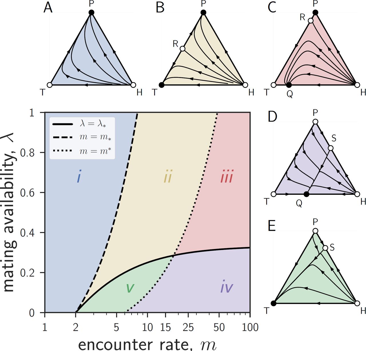
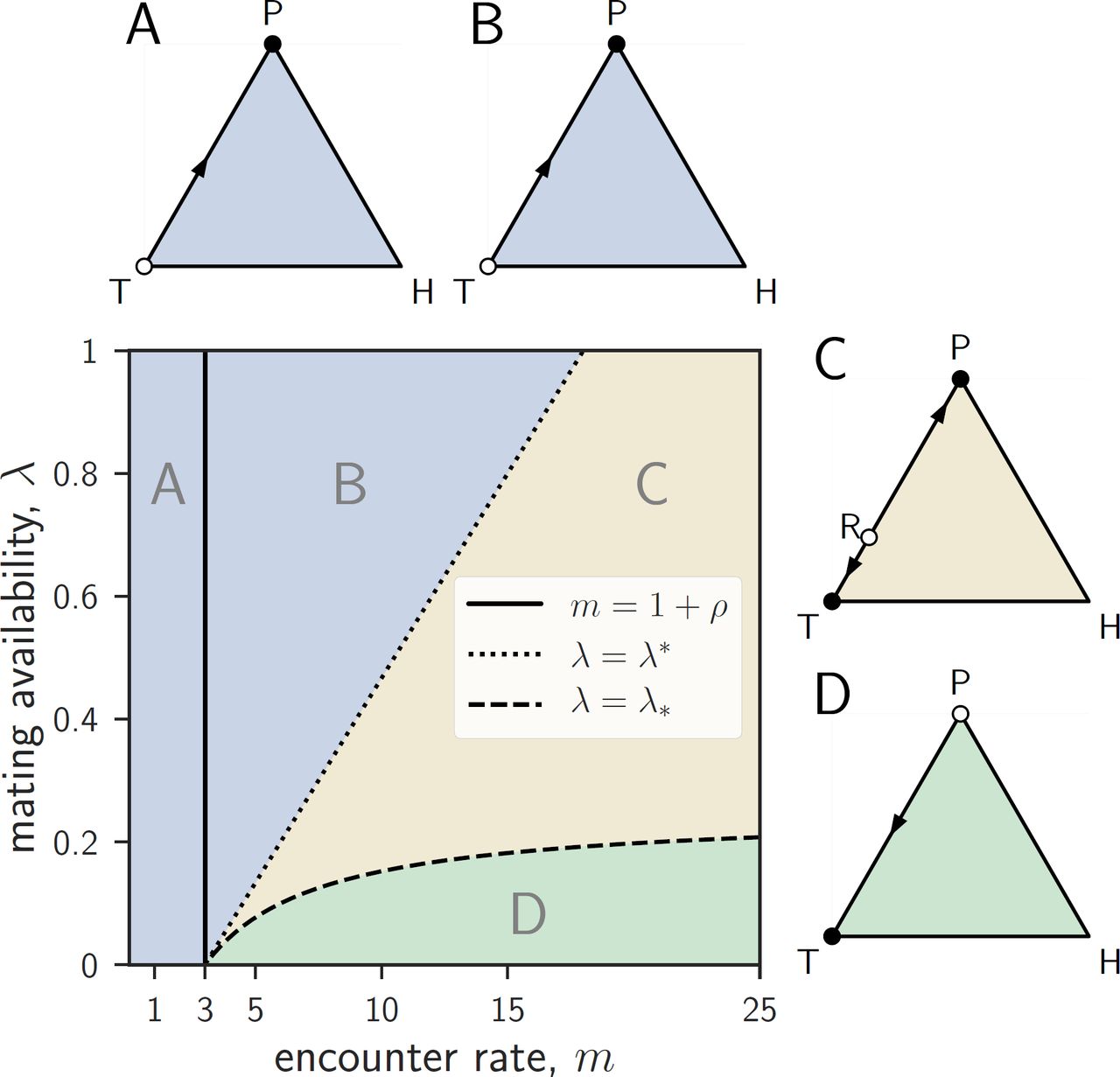
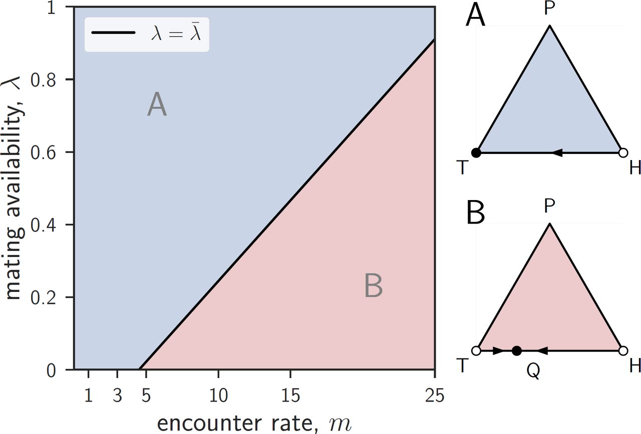