

Abstract
Cognitive models are a fundamental tool in computational neuroscience, embodying in software precise hypotheses about the algorithms by which the brain gives rise to behavior. The development of such models is often largely a hypothesis-first process, drawing on inspiration from the literature and the creativity of the individual researcher to construct a model, and afterwards testing the model against experimental data. Here, we adopt a complementary data-first approach, in which richly characterizing and summarizing the patterns present in a dataset reveals an appropriate cognitive model, without recourse to an a priori hypothesis. We apply this approach to a large behavioral dataset from rats performing a dynamic reward learning task. The model revealed suggests that behavior on this task can be understood as a mixture of three components with different timescales: a quick-learning reward-seeking component, a slower-learning perseverative component, and a very slow “gambler’s fallacy” component.
Introduction
A fundamental goal of cognitive neuroscience is to understand the algorithms by which the brain gives rise to behavior. One of the fundamental tools used in this pursuit is cognitive modeling. This involves constructing software agents which are capable of performing tasks, and tuning them such that their behavior matches as closely as possible the behavior of human or animal subjects. The software algorithms of these agents then constitute precise hypotheses about the neural algorithms used by the brain to perform the same tasks (O’Doherty et al. 2007; Corrado & Doya 2007; Daw 2011). Cognitive models have been used to shed light on the neural mechanisms of many aspects of cognition, including learning (Daw & Doya 2006; Lee et al. 2012), memory (Norman et al. 2008), attention (Heinke & Humphreys 2005), and both perceptual (Gold & Shadlen 2007; Hanks & Summerfield 2017) and value-based (Sugrue et al. 2005) decision-making.
The process by which new cognitive models are constructed is often largely hypothesis-driven. One popular and successful approach, for example, draws inspiration from an appeal to optimality, looking to algorithms which are provably the best solutions that exist for some particular problem (Gold & Shadlen 2002; Körding 2007; Griffiths et al. 2015). Another draws inspiration from artificial intelligence, looking to algorithms which are successful in practice at solving a wide variety of problems (Daw & Doya 2006; Dayan & Niv 2008). These and other hypothesis-first approaches have been extremely productive, but studies following them are subject to two important limitations. The first is that they typically consider a relatively small number of models, and are able to determine that a particular model is the best of the set, but not that it is good in an absolute sense or that it recapitulates the neural algorithm (Daw 2011). The second is that the development of new models is dependent on inspiration from adjacent fields or on the creativity of the individual researcher, limiting the pace of hypothesis generation.
In many fields, recent decades have seen methodological advances that enable the collection of very large datasets, and the mining of those datasets to reveal unexpected patterns (e.g. Hardy & Singleton 2009). These tools have enabled data-first approaches to hypothesis generation, which have proven an important complement to hypothesis-first methods in these fields (Kell & Oliver 2004). Behavioral neuroscience too has seen methodological advances which enable the collection of larger and richer datasets (Schaefer & Claridge-Chang 2012; Gomez-Marin et al. 2014), raising the hope that similar data-first methods might hold promise for the development of cognitive models.
Here, we take advantage of one of these advances: the development of high-throughput methods for studying decision-making in rats (Erlich et al. 2011; Brunton et al. 2013). We use this tool to collect a large behavioral dataset from rats performing a classic reward-guided learning task, the “two-armed bandit” task (Samejima et al. 2005; Daw et al. 2006; Ito & Doya 2009; Kim et al. 2009). We adopt a data-first approach to reveal the patterns that are present in this dataset. We show that these patterns can be summarized by a relatively compact model, with a small number of free parameters, and that this model can be viewed as a cognitive model, describing a candidate for the neural algorithm implemented by the rat brain to solve the task. When viewed in this way, the model suggests that behavior results from three distinct mechanisms with different timescales – a reward-seeking mechanism that considers only the most recent few trials, and tends to repeat choices that led to rewards and switch away from those that did not; a perseverative mechanism that considers a slightly longer history, and tends to repeat choices regardless of their outcomes; and a “gambler’s fallacy” mechanism that considers many tens of trials, and tends to repeat choices that did not lead to rewards. Each of these components was present consistently across rats, with rat-by-rat variability in their precise strengths, timecourses, and other parameters. The first (reward-seeking) component is consistent with popular cognitive models and predicted by existing theory, but the second two (perseverative and gambler’s fallacy) components are to our knowledge unexpected.
Results
Task
Rats performed a probabilistic reward learning task (the “two-armed bandit” task; Ito & Doya 2009; Kim et al. 2009; Sul et al. 2010) in daily sessions (20 rats; 1,946 total sessions; 1,087,140 total trials). In each trial, the rat selected one of two nose ports and received either a water reward or a reward omission (Figure 1a). The probability of reward at each nose port evolved slowly over time according to a random walk (Figure 1b). Task performance therefore required continual learning about the current reward contingencies, and selecting the port with the higher reward probability. The rats performed well at this task, tending to select the nose port that was associated with a higher probability of reward (Figure 1c). Importantly, rats’ performance did not match that of an optimal agent (Figure 1c, see Methods), meaning that we can expect to find patterns in their behavior that are not purely a function of the task itself, but rather of the strategy with which the rats approach it.

A) On each trial, rat selects one of two possible choice ports. B) Probability of reward at each port evolves over time according to an independent random walk. C) Rats tend to select the port with the higher reward probability. Their performance does not match that of an ideal observer model.
Unconstrained Models
First, we consider predictive models which characterize the relationship between a rat’s choice behavior and recent history of choices and rewards in a very general way. For these (and all other) models, we choose to model the rats choice on each trial, using as predictors the recent history of choices and their outcomes. These “unconstrained” models attempt to predict the choice on trial t using the full history of choices and rewards on trials t – 1 through t – n (n-markov models; Ito & Doya 2009). Specifically, we label the choice made (left or right) and the outcome received (reward or omission) on trial t as Ct and Ot, respectively, and we define the history, H, as matching between a pair of trial if the choices and outcomes that preceded those trials are identical within a window of N trials:
 where δ is the Kroenecker delta, which takes on a value of one when its arguments match and zero otherwise. The predicted choice probability for each trial is then determined by the fraction of trials with matching histories in which the rat selected each port:

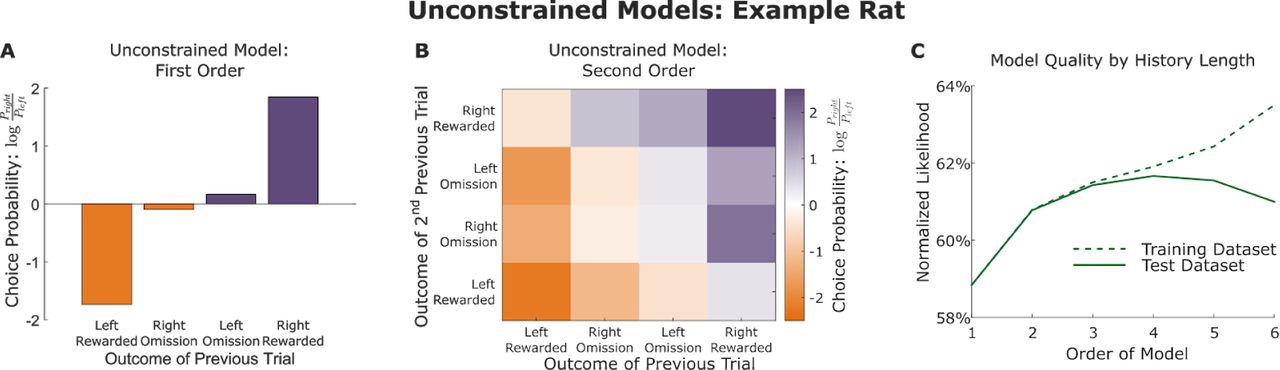
Predicted choice probabilities for an example rat for N=1 and N=2 are shown in Figure 2. The unconstrained model introduces no assumptions about the way in which recent past choices and outcomes influence future behavior. The cost of this flexibility is a large number of effective free parameters: one per possible history H. Since each trial can be one of four types (left/right choice, reward/omission), this amounts to 4N total parameters. We evaluate the performance of the model by computing a normalized likelihood score (Daw 2011), using two-fold cross-validation. We find that cross-validated likelihood is similar to training-set likelihood for short history windows, but decreases for longer windows as the number of free parameters increases beyond what the dataset is able to meaningfully constrain (Figure 2C). In the range where the unconstrained model’s cross-validated and training likelihoods are similar (N ≲ 4), we can be confident that the model is not substantially overfitting, and use it as a standard against which to evaluate other models. No model that considers only recent choices and rewards as predictors is more flexible than the unconstrained model, so its likelihood provides a ceiling on the performance that can be expected from any such model, given the entropy of the data.

A) Unconstrained model of order one, fit to a dataset from an example rat. This model consists of log choice probability ratios for trials immediately following a trial of each of the four possible trial types. B) Unconstrained model of order two for the same example rat. This model makes separate predictions for trials following each possible pair of trial types, resulting in sixteen total choice probabilities. C) Quality of fit for unconstrained models of orders one through six for the example rat. Normalized likelihood was computed using cross-validation, and likelihoods for both the fit datasets (training dataset) and the held-out datasets (testing dataset) are plotted. Likelihoods are similar for both datasets when the order is small.
Linear models
Next, we consider predictive models which attempt to mitigate overfitting by introducing an assumption about the way in which past trials choices and outcomes affect future behavior. In particular, these models assume that each past trial exerts an influence on future choice that is independent of the influence of all other past trials. The influence of each past trial is summed, and this sum is used to compute choice. The most general models in this family fit the relationship of the sum to future choice (linear-nonlinear-poisson models; Corrado et al. 2005), but we consider here models which additionally assume that this relationship is well-approximated by a logit function (logistic regression models; Lau & Glimcher 2005). For our task, the most general of these models can be written as:

where Ct is the choice made on trial t (coded as +1 for right and −1 for left), Ot is the outcome received (+1 for a reward and −1 for an omission), and the βs are fit weighting parameters. Like the unconstrained models, these models consider a history of N recent trials, but unlike them, they do not assign a parameter to each possible history. Instead, they assign a set of weights to each slot within that history, quantifying the effect on upcoming choice when a trial of each type occupies that slot. In our model, these weights are organized into three vectors: βX, which quantifies “reward seeking” behavior in which the animal tends to repeat choices that lead to rewards and to switch away from choices that lead to omissions; βC, which quantifies a “choice perseveration” pattern in which the animal tends to repeat past choices without regard to their outcomes; and βO, which would quantify a main effect in which outcomes affected choice, without regard to the side on which they were delivered.
Fits of the linear model reveal large and consistent effects of reward seeking and choice perseveration, and relatively weak and inconsistent main effects of outcome (example rat: Figure 3A; all rats: Figure S1). These fits were relatively resistant to overfitting: normalized likelihoods of the linear model for the testing and training datasets diverged from one another at much larger N than those of the unconstrained model (Figure 3B, compare to Figure 2B). This resistance to overfitting comes at the cost of the assumption that past outcomes contribute linearly to current choice. One way to test this assumption is to compare the likelihood scores of the unconstrained and the linear models directly: if the additional flexibility of the unconstrained model allows it to achieve a higher score, then meaningful nonlinear interactions must exist in the dataset. We find that the linear and the unconstrained model earn similar likelihood scores up to N ≈ 4, and that for larger N the linear model achieves larger scores (Figure 3C). This partially validates the idea that past choices and outcomes contribute to present choice in a linear way. It rules out strategies incorporating nonlinear interactions within the most recent few trials (e.g. “repeat my choice unless I get two omissions in a row, then switch”), but not those incorporating longer-term nonlinear interactions exist (e.g. “if my most recent choice matches my choice from six trials ago, repeat it”). In addition to partially validating the linearity assumption, these results provide a standard against which to evaluate other models which also incorporate a linearity assumption of this model. No such model is more flexible than the linear model, so its likelihood score provides a ceiling on the performance that can be expected, given the entropy of the data.
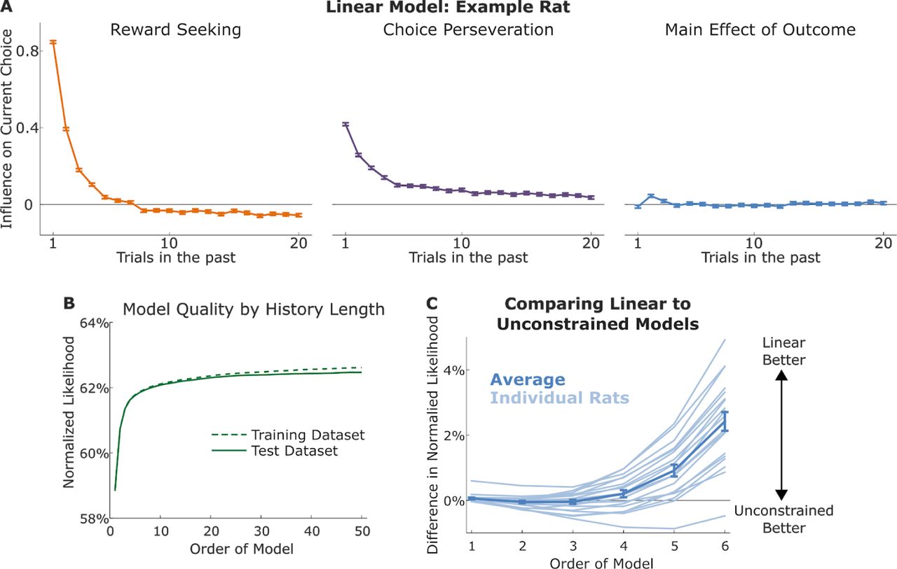
A) Linear model of order twenty, fit to the example rat. The model consists of three sets of weights characterizing the influence of past trials on current choice. Reward-seeking weights (left) characterize the tendency to repeat choices that led to rewards and switch away from choices that led to omissions; perseveration weights (middle) characterize the tendency to repeat past choices regardless of their outcomes; outcome weights (right) characterize the tendency for outcome (reward/omission) to influence choice regardless of the choice that led to it. B) Quality of model fit for the example rat, as a function of the order of the model (number of past trials considered). Normalized likelihood was computed using cross-validation, and likelihoods for both the fit datasets (training dataset) and the held-out datasets (testing dataset) are plotted. Likelihoods are similar for both dataset up to relatively larger order (compare to Figure 2C). C) Difference in normalized cross-validated likelihood between linear and unconstrained models of the same order. Quality of fit of the linear model approximates or exceeds that of the unconstrained model for all orders.
Reduced linear models
Inspecting the fit weights of the linear models (Figure 3a, Figure S1), several patterns are apparent. For all rats, reward-seeking weights are large and positive for the most recent few trials (Figure 3A, left), while perseverative weights were smaller, but extended further back in time (Figure 3A, middle). Outcome weights were small and showed patterns that were inconsistent across rats (Figure 3A, right). In all cases, weights for very recent trials were relatively large, while weights for trials in the distant past were relatively small. We sought to capture these patterns using a “reduced linear model” comprising a mixture of exponential processes along with a set of weights associated with the most recent trial. Each exponential process was characterized by an update rate α, determining how far into the past that exponential process extended, as well as two weighting parameters wc and wx, determining how strongly that process was influenced by perseveration and reward-seeking. These parameters govern the evolution of a hidden variable S, which was set to 0 on the first trial of each session and updated on each trial according to the following rule:

Choice probability on each trial was determined by summing the influence of each of the exponential processes, as well as the influence of the most recent trial:

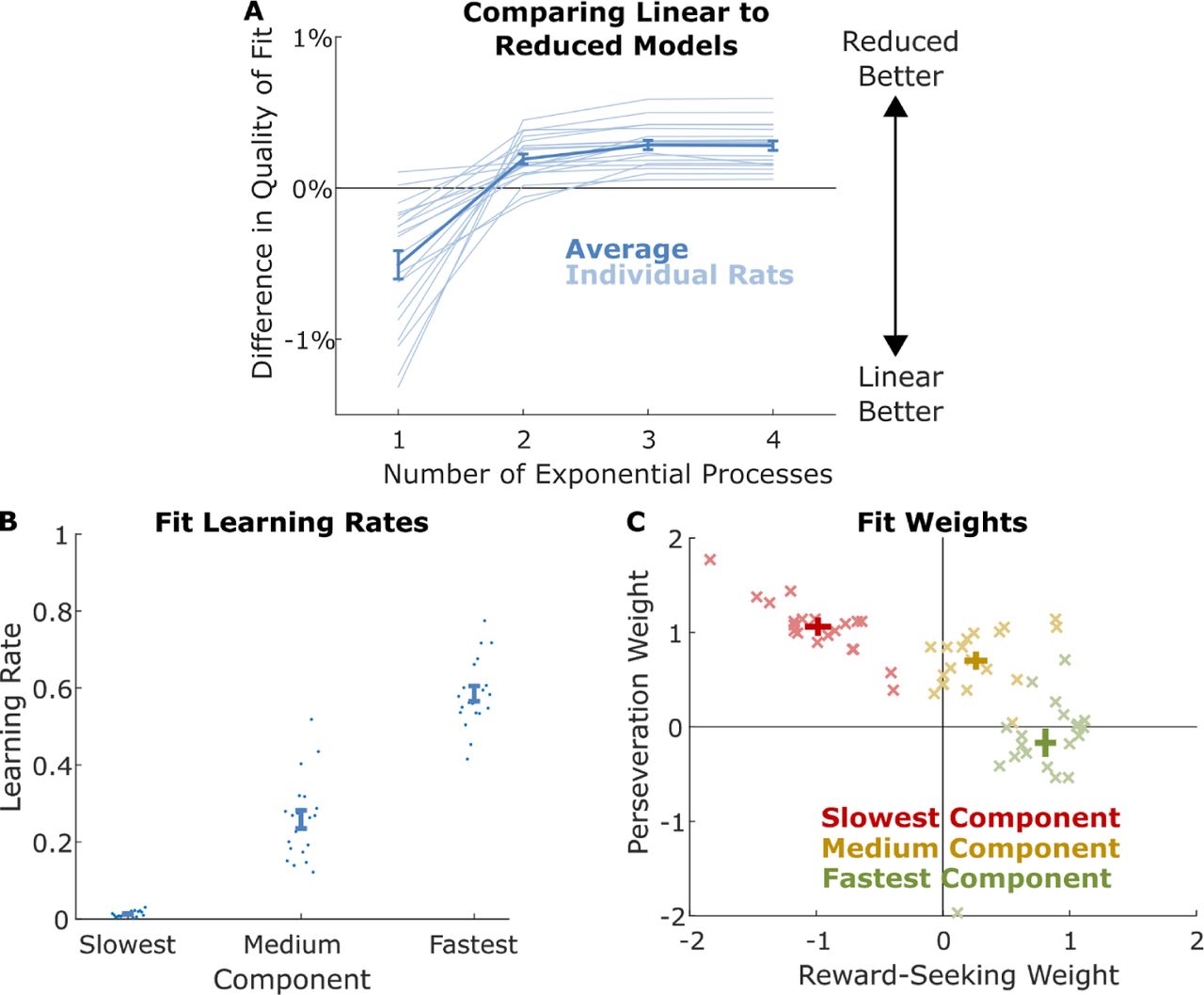
We compared the quality of fit of the reduced model to the quality of fit of the best linear model for each rat, as a function of the number of exponential processes included (Figure 4A). We found that that the dataset from each rat was best explained by a mixture of exactly three exponential components: Limiting the model to only two components resulted in a decrease in quality of fit for each rat (mean difference in normalized likelihood 0.1, sem 0.2, p=10−4), while allowing the model to use four components did not result in an increase in quality of fit (mean difference in normalized likelihood −0.004, sem 0.004, max 0.006, p=0.3).
A) Difference in normalized cross-validated likelihood between reduced model with different numbers of exponential processes and the best linear model for each rat. Quality of fit of reduced model increases until three processes are included, and then does not continue to increase. Reduced model with three processes narrowly outperforms the best linear model. B) Weights of three-component reduced models fit to each rat’s dataset. Weights are color-coded by whether they belong to the component with the fastest, middle, or slowest learning rate for that rat.
For this reason, we consider fits of the model with exactly three components. We found that such a model outperformed the best linear model for each rat (mean difference in normalized likelihood 0.28, sem 0.03, p=10−4, signrank test; Figure 4A). Learning rates (Figure 4B) were, by selection, largest for the first component (mean 0.59, sem 0.02), smaller for the second component (mean 0.26, sem 0.02), and smallest for the final component (mean 0.01, sem 0.002). Weights are colored by whether the component they belong to has the largest, medium, or smallest learning rate of the three components belonging to that rat. We find a pattern of fit weights for each component that is strikingly consistent across rats. The component with the fastest learning rate (Figure 4C, green points) was dominated by a reward-seeking pattern – the reward-seeking weight was positive for every rat (mean 0.81, sem 0.06), while the perseverative weight was inconsistent in sign and much smaller (mean −0.17, sem 0.12). The component with the medium learning rate (Figure 4C, yellow points) was dominated by a perseverative pattern – the perseverative weight was positive for every rat (mean 0.70, sem 0.06), while the reward-seeking weight was inconsistent in sign and much smaller (mean 0.26, sem 0.07). The component with the slowest learning rate (Figure 4C, red points) had a negative reward-seeking weight (mean −0.99, sem 0.08) and a positive perseverative weight (mean 1.1, sem 0.07) for each rat. Moreover, the reward-seeking and perseverative weights for this component were approximately equal in magnitude, though opposite in sign (mean sum 0.08, sem 0.04). Equal and opposite weights for reward-seeking and perseveration cancel one another’s influence following rewarded trials (perseveration seeks to repeat the choice, negative reward-seeking seeks to switch it), but reinforce one another following omission trials (perseveration and negative reward-seeking both seek to repeat the choice). This results in a lose-stay (“gambler’s fallacy”) pattern of behavior which ignores rewards and seeks to repeat choices that led to omissions.
In sum, fits of the reduced model reveal three components of behavior with different timescales. The fastest component is dominated by a pattern of reward-seeking, though modulated by perseveration in a way that is idiosyncratic to individual rats. The next component is dominated by a pattern of perseveration, though modulated by reward-seeking in a way that is idiosyncratic to individual rats. The slowest component is a “gambler’s fallacy” pattern which tends to repeat choices that lead to omissions. Individual rats are characterized by different time constants, weights, and modulations for each of these patterns, but the same three patterns are present in each.
Reduced Model: Cognitive Formulation
Finally, we seek to express the behavioral patterns revealed by the reduced model by rewriting this model using notation typical of cognitive models. We will write this as a mixture-of-agents model, in which each rat is modeled as a mixture of three independent agents following different strategies: a reward-seeking agent, a perseverative agent, and a gambler’s fallacy agent.
The reward-seeking agent represents an estimated relative reward value V. This quantity is initialized to zero at the beginning of each session, and updated after each trial according to the following rule:

In the case that εv is much smaller than one, this approximates an estimate of the relative value of the two reward ports, computed by a mechanism similar to the delta rule found in temporal difference reinforcement learning models (Sutton & Barto 1998). It is also equivalent to an exponential process as in equation 3, with wx equal to one, and wc equal to εv.
The perseverative agent represents a relative perseverative strength H, which is initialized to zero at the beginning of each session, and updated after each trial according to:

In the case that εh is much smaller than one, this is equivalent to a recency-weighted estimate of how often each port has been chosen. It is also equivalent to an exponential process with wc equal to one and wx equal to εh. This mechanism is similar to a process of Hebbian plasticity which strengthens the representations of recently taken actions – a mechanism which has been proposed to underlie habitual behavior (Ashby et al. 2010; Miller et al. 2016).
The gambler’s fallacy agent represents an internal variable G. It is initialized to zero at the beginning of each session, and updated after each trial according to:

In the case that εg is much smaller than one, this represents a recency-weighted average of the relative number of losses incurred at each port. This is equivalent to an exponential process with wc equal to 1 − εh, and wx equal 1 + εh, and wo equal to zero.
The action of the model on each trial is determined by a weighted average of V, H, and G:

A complete set of parameter equivalencies between this cognitive formulation of the reduced model and the exponential formulation (Equations 3 and 4) is given in Table 1. Weights for each agent (β) were positive for each rat (reward-seeking: mean 0.81, sem 0.06; perseverative: mean 0.7, sem 0.06; gambler’s fallacy: mean 1.0, sem 0.07; all P=10−4, signrank test). Modulations for each agent were smaller than one for nearly all agents (reward seeking: 19/20, p=0.001; perseverative: 18/20, p=0.002; gambler’s fallacy: 20/20, p=10−4), and had signs which varied across rats (reward-seeking: 7/20 positive, p=0.11; perseverative: 17/20 positive, p=0.001; gambler’s fallacy: 11/20 positive, p=0.12).
Parameter equivalencies between a reduced model with three exponential processes and a cognitive formulation of the same model.
Discussion
We trained rats to perform a reward-learning task in which they repeatedly selected between two ports with constantly-changing probabilities of reinforcement, and we sought to build a cognitive model capturing the patterns in their behavior. This work adds to a large body of previous work modeling behavior in tasks of this kind (Samejima et al. 2005; Daw et al. 2006; Kim et al. 2009; Ito & Doya 2009), building on it by collecting a large behavioral dataset, and by adopting a data-first modeling approach to reveal patterns in the dataset in a hypothesis-neutral way.
In keeping with this literature, we built models which sought to predict the choice of the subject on each trial, using as predictors the history of choices made and rewards received on recent trials. In making this decision, we choose to ignore (treat as noise) all other factors that might influence choice, including factors such as satiety or fatigue that may play an important role in modulating behavior. We began by fitting the most general model possible that are consistent with this choice, the unconstrained models, to establish a ceiling on the possible quality of model fit – since no model in the class is more flexible, no such model can outperform the unconstrained model in terms of fit quality. In the regime where the unconstrained model does not overfit, this ceiling is also a useful benchmark – any model which accurately captures the generative process should fit the data approximately as well as the unconstrained model. An important precedent to this benchmarking step is found in Ito & Doya (2009), who similarly fit unconstrained models, and compared them to several cognitive models. Our work adds to this by comparing training-dataset and testing-dataset performance to determine the range in which these models establish a valid benchmark, and by utilizing a much larger dataset, allowing us to establish a benchmark for models considering up to three or four past trials.
With this benchmark in hand, we fit a set of models with an additional constraint of linearity – these models assume that each past trial to contributes independently to present choice. The performance of the linear models matches the benchmark in the regime in which the benchmark is valid, suggesting that the true generative algorithm may be one that respects this constraint. These linear models have an important precedent in earlier work (Corrado et al. 2005; Lau & Glimcher 2005), which used similar models to characterize behavioral data from primates performing reward-guided decision tasks. Our work goes beyond this in that it validates these models with respect to the benchmark from the unconstrained models, and in that it distills these patterns further into a reduced model, and showing that this reduced model can be viewed as a cognitive model.
Fits of the linear model indicate that rats have strong tendencies of “reward-seeking” (repeat past choices that led to reward, switch from those that did not) and “perseveration” (repeat past choices without regard to outcome), and that events in the recent past have a stronger influence on choice than events that are more remote. We sought to compress these patterns using a model that assumes the linear patterns can be understood as arising from a mixture of several exponential processes with distinct weights. Strikingly, we found that the dataset from each rat was best modeled as arising from a mixture of exactly three exponential processes, and that the weights of each of these showed consistent patterns across rats. The fastest process (timecourse ∼3-5 trials) was predominantly a pattern of reward-seeking, while the middle process (timecourse ∼5-10 trials) was predominantly one of perseveration. The slowest process (∼tens or hundreds or trials) was consistent with a “gambler’s fallacy” pattern that tends to repeat choices which have led in the past to losses. Finally, we rewrote this reduced exponential model using notation typical of cognitive models, making explicit the nature of each of the three components. Expressing the model in this cognitive form converts it from a tool for characterizing the patterns present in a behavioral dataset into a precise hypothesis about the mechanisms by which that behavior was produced. This hypothesis makes testable predictions for future experiments: that the trial-by-trial variables (V, H, and G) associated with each process must be represented in the brain and updated trial-by-trial, and that different neural mechanisms might underlie each of the three processes. The first set of predictions might be tested by experiments that record neural activity during task performance, and the second by experiments that inactivate (or otherwise perturb) neural activity in different brain regions.
The first, reward-seeking, component of the model is consistent with a long body of literature on reward-guided decision making, beginning with Thorndike’s “law of effect”, which holds that actions that have led to reward in the past are likely to be repeated in the future (Thorndike 1911). It is reminiscent of popular reinforcement learning algorithms, such as the temporal difference rule (Sutton & Barto 1998), which are commonly used to model behavior on tasks of this kind (Barraclough et al. 2004; Daw et al. 2006; Kim et al. 2009). These algorithms are similar to our exponential process in that they maintain a cached variable, updating it on each trial by taking its weighted average with a value from that trial’s observation. They are different in that they typically maintain one cached value per possible action, while our process caches only a single value, representing the relative history of recent outcomes at each port.
Perseveration in reward-guided tasks has been observed in a wide variety of tasks and species (Lau & Glimcher 2005; Lee et al. 2005; Ito & Doya 2009; Kim et al. 2009; Rutledge et al. 2009; Balcarras et al. 2016). One common way of modeling it is to consider it as arising from some modulation to a reward-seeking process – for example using different learning rates for positive and negative outcomes (Ito & Doya 2009), or by fitting a perseverative weight that considers only the immediately previous trial (Daw et al. 2011). Our results suggest that perseveration results from a process that is separable from reward-seeking (having its own timecourse), and that it considers a relatively large number of past trials. The idea of a perseverative process considering a relatively long behavioral history is consistent with Thorndike’s second law, the “law of exercise”, which holds that actions which have often been taken in the past are likely to be repeated in the future (Thorndike 1911). It is also consistent with ideas from the literature on the psychology of habit formation (Dickinson 1985; Graybiel 2008; Ashby et al. 2010; Wood & Rünger 2016), which propose that habits are fixed patterns of responding that result from simple repetition of past actions (for further discussion, see Miller et al. 2016; Miller et al. 2018)
Acknowledgements
We would like to thank Alex Piet, Kim Stachenfeld, Nathaniel Daw, Yael Niv, Bas van Ophuesden, Chuck Kopec, and Jeff Erlich for helpful discussions.
References


