

Abstract
High-throughput chromosome conformation capture (Hi-C) experiments are typically performed on a large population of cells and therefore only yield average numbers of genomic contacts. Nevertheless population Hi-C data are often interpreted in terms of a single genomic structure, which ignores all cell-to-cell variability. We propose a probabilistic, statistically rigorous method to infer chromatin structure ensembles from population Hi-C data that takes the ensemble nature of the data explicitly into account and allows us to infer the number of structures required to explain the data.
In recent years, chromosome conformation capture (3C) methods have emerged as a powerful tool to investigate the three-dimensional organization of genomes on previously inaccessible length scales. Thanks to experimental advances and decreasing sequencing costs, genome-wide 3C methods such as Hi-C (1) and Hi-C variants (2; 3) have yielded contact maps with resolutions of up to 1 kb. High-resolution contact maps have provided fascinating insights into the organization of chromatin domains and compartments of various sizes and their role in gene regulation (1; 4; 5; 6; 3).
Although Hi-C can be performed in single cells (7; 8; 9; 10; 11), much richer data are usually ob-tained by analyzing populations of cells at the price of a more difficult interpretation of the data: Contact maps obtained in population Hi-C experiments show an average over millions of cells. Given that single-cell Hi-C experiments revealed significant structural variability among cell nuclei (7), it remains difficult to assess the information content and degree of structural heterogeneity reflected by population Hi-C data.
Much effort has gone into the development of chromatin structure determination approaches, in which a single consensus structure is calculated (12). In light of recent results on cell-to-cell variability and considering experimental limitations and biases, consensus structure approaches are fundamentally limited, if not flawed (13). Several approaches taking into account the heterogeneity of cell popu-lations have been explored. Matrix deconvolution has been used to unmix Hi-C matrices without explicitly modeling 3D structures (14; 15). While some structural information is already apparent in contact matrices, it is useful to find an approximate 3D representation giving rise to the data. For example, a 3D chromosome model allows the detection of three-way interactions not accessible in 3C data (16). Furthermore, data from other sources (e.g., imaging) can be included in the modeling process. A second approach is thus to calculate an ensemble of structures that reflect the structural heterogeneity of chromosomes more realistically than consensus structure approaches and reproduce the contact map only on average. This can be achieved in two different ways: First, one can optimize a set of structures generated from a polymer model so as to reproduce, on average, the experimental data (2; 17; 18; 19). A second possibility is to adjust the parameters of a polymer model such that by simulating the polymer model an ensemble of structures is obtained that reproduces the experimental data on average (20; 21; 22).
In this communication, we extend the scope of our previous work on Bayesian chromosome struc-ture inference from single-cell Hi-C data (23) to population-averaged contact data, combining the explicit modeling of chromatin structure populations with a rigorous probabilistic interpretation of the data. We leverage the full power of Bayesian inference to compute multi-state models of chromo-some structures, which together reproduce the population contact data.
Our approach is based on the Inferential Structure Determination (ISD) (24, Supplementary Notes) framework. ISD infers a structural model x along with unknown modeling parameters α from experi-mental data D and background information I. The inference problem is solved by sampling from the joint posterior distribution for x and α, conditioned on D and I, which can be expressed using Bayes’ theorem as
 Here we assume that a single structure x can explain the data D, as is the case for, e.g., proteins with a stable and unique fold. Sampling from Pr(x, α|D, I) results in a statistically well-defined ensemble of structures with associated estimates of nuisance parameters α, each being assigned a probability given by the posterior distribution.
To accommodate the fact that most 3C experiments are performed on populations of molecules with possibly very different conformations due to cell-to-cell heterogeneity and dynamics, we extend the scope of the ISD approach to the inference of multi-state models X = (x1, …, xn) consisting of n structures xk. The central quantity in this extended ISD framework is the posterior distribution
 sampling from which results in a hyperensemble, that is, a representative set of multi-state models Xi with associated nuisance parameters αi, in which each pair (Xi, αi) has a probability given by Equation 2. In the case of a single state (n = 1), we recover the original ISD formulation and infer a consensus structure.
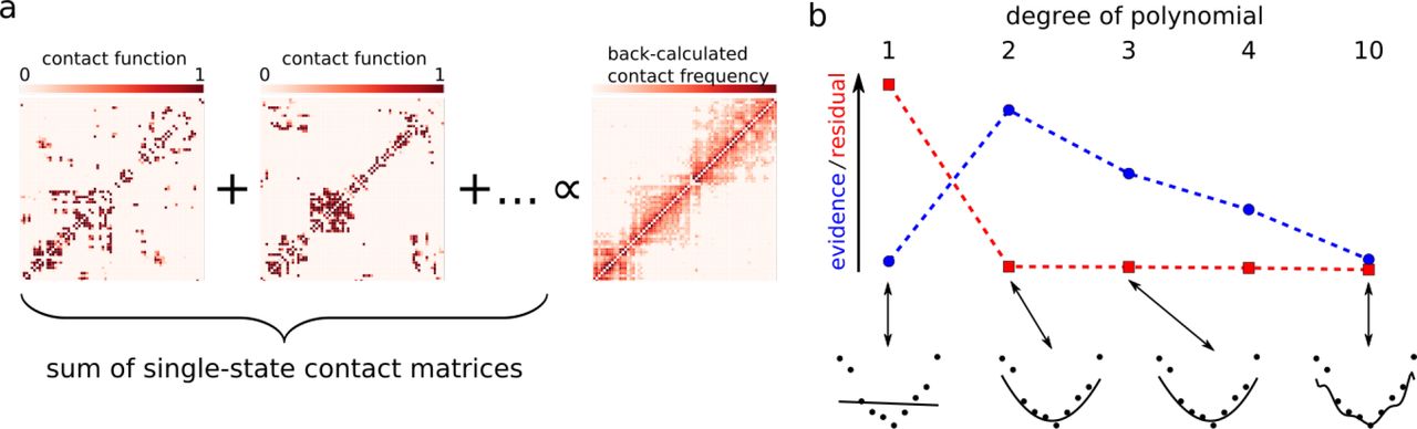
At the center of a Bayesian approach is a generative model for the data Pr(D|X, α, n, I) given a set X of n structures. Our generative model is based on a forward model to compute average contact matrices, which are idealized, noise-free data. As shown in Figure 1a, each structure xk that is part of X gives rise to a smoothed contact matrix based on a threshold distance. The n contact matrices are summed together and multiplied with a scale factor α that is estimated from the data. We model deviations from these idealized data due to experimental noise, forward model inaccuracy and, in case of Hi-C data, data normalization with Poisson distributions whose rates are given by the idealized count data.

Main components of the proposed chromatin structure inference approach. (a)Forward model to calculate idealized contact frequency matrices from structures that are part of a multi-state model. The contact matrices arising from each structure are summed together and multiplied with a scaling factor to yield the backcalculated contact frequency matrix on the right. (b)Bayesian model comparison illustrated for a polynomial curve fitting example. Shown is the evidence (blue) and the residual mismatch between model and data (red) for polynomials of increasing degree. Data points and best fitting models are shown below the x axis.
Under reasonable independence assumptions, the joint prior distribution Pr(X, α|n, I) factorizes and we can formulate separate prior distributions for all states (x1, …, xn) and for the scale factor α. We model the physical interactions within a single structure xk by a coarse-grained beads-on-a-string model similar to our model for single-cell data (23). Further details on our statistical model for population-averaged contact data and our choice of prior distributions are explained in Supplementary Notes.
We use a range of Markov Chain Monte Carlo (MCMC) techniques to address the challenging task of sampling from Pr(X, α|n, D, I) (see Supplementary Notes for details). Once representative samples have been drawn from the posterior distribution, the structure determination problem is solved and the estimated multi-state models can be analyzed.
A crucial parameter in all structure calculation methods that model explicit ensembles (2; 17; 18) is the number of states n. Existing multi-state modeling approaches choose n in an ad hoc man-ner. For example, in the GEM (18) software, the default value for n is four and differs largely from n = 10000 used by Alber and coworkers (17). From a Bayesian perspective, the number of states n is a model parameter that should be inferred from the data. Depending on the true heterogeneity of the chromosome structures n will adopt smaller or larger values. If n is too small, we underfit the contact data resulting in highly strained structural models. If n is too large, the structures of the states are only loosely defined and potentially overfit the contact data. Therefore, a simple goodness-of-fit criterion is not sufficient to select n. We have to balance goodness-of-fit against model complexity. Figure 1b illustrates this point for polynomial curve fitting. The degree of the polynomial determines the flexibility of the fitting function and therefore corresponds to the number of states n. For data generated from a parabola, the goodness-of-fit reaches an optimum if we use polynomials of degree two and higher eventually resulting in overfitting: the fitted curve closely follows each data point.
A unique feature of Bayesian data analysis is that it offers an objective, albeit computationally often challenging framework for model comparison (25). Our belief in a particular choice of n is encoded by the posterior probability

Assuming that a priori all n are equally likely, the ratio of two choices for the number of states n and n′ can be written as

The odds ratio Onn′ is called the Bayes factor and tells us which model to prefer: for Onn′ > 1, an n-state model describes the data better; while Onn′ < 1 indicates a preference for a model based on n′ states. The model evidence Pr(D|n, I) has a built-in penalty for model complexity. In the curve fitting example (Figure 1b), Pr(D|n, I) selects the correct degree of the polynomial (n = 2), although polynomials of degree > 2 achieve a better fit. This is because with increasing degree also the number of curves that do not fit the data increases, which is reflected by a decrease in the model evidence. The evaluation of the model evidence involves calculating two possibly intractable and high-dimensional integrals, which in all but the most trivial cases have to be approximated numerically. As several of the occurring distributions are of a non-standard form, we use histogram reweighting (26; 27) to approximate the evidences.
We implemented our method in a freely available Python package (http://bitbucket.org/simeon_carstens/ensemble_hic). As a proof of concept, we first apply our inference approach to contact data simulated from two protein structures. We consider beads-on-a-string models of two protein domains, the B1 immunoglobin-binding domain of streptococcal protein G (PDB identifier 1PGA) and the SH3 domain of human Fyn (PDB identifier 1SHF). Only positions of Cα atoms were taken into account, and the SH3 domain was truncated by three C-terminal residues to match the length of 1PGA. This results in two very different conformations of a chain of 56 beads (Figure 2a,b). We generated simulated contact frequencies and used ISD to infer representative multi-state models. We simulated the posterior distributions for n = 1, 2, 3, 4, 5, 10 states. Model comparison shows that the model with n = 2 states is strongly preferred, as indicated by P (D|n = 2, I)/P (D|n = 1,I) > 10307 and P (D|n = 2,I)/P (D|n = 3,I) > 10160 (Figure 2c). It is reassuring that while the evidence de-creases for n > 2, models with an even number of states are preferred over models with a similar, but uneven number of states. The reason for this is that for even n, half of the states adopt the confor-mation of the B1 domain and the other half adopts the conformation of the SH3 domain, thus having few superfluous parameters (Supplementary Figure S1). For uneven n, on the other hand, there is at least one superfluous state (Supplementary Figures S2 and S3), contributing uninformative parameters which are penalized in the evidence. We find that, for n > 2, the average scale factor α decreases monotonically with an increasing number of states (Figure 2f), in agreement with our intuition that α compensates for the smaller number of simulated states as compared to typical numbers of counts in the data.

Reconstruction of protein structures from simulated data. (a), (b)Reference structures of the SH3 domain (a) and protein G (b). (c) Model evidences for different number of states. (d), (e) “Sausage representation” of reconstructed folds (n = 2 states). Tube thickness indicates the local precision of bead positions. (f)Average values of sampled scale factor.
Figure 2d,e shows the two reconstructed states from the n = 2 simulation which deviate from the ground truth by an root-mean-square deviation of bead positions (RMSD) of (1.46 ± 0.11) Å for the B1 domain and (1.59 ± 0.21) Å for the SH3 domain. ISD thus recovers both conformations to very good accuracy.
Having established the validity of our approach on simulated data, we now apply our extended ISD approach to a 5C dataset covering the X-inactivation center in mouse embryonic stem cells (mESCs)(5). We restrict our analysis to contact frequencies between primer sites within the two consecutive TADs harbouring the Tsix and Xist promoters, respectively, and their boundary region. Similar to previous work on the same data (20), we model the corresponding ~920 kb region by M beads, each represent-ing a genomic length of ~ 920/M kb. To keep the computational efforts for sufficient MCMC sampling reasonable, we chose a rather coarse resolution with one bead representing 15 kb, resulting in a total of 62 beads. Simulating the ISD posterior distribution for n = 1, 5, 10, 20, 30, 40, and 100 states and calculating model evidences, we find that the multi-state model with n = 20 states is clearly preferred by the data (Figure 3a). This result establishes that Bayesian model comparison is indeed able to determine a unique, optimal number of states for 5C data. The low resolution of these simulations lets us expect limited biological meaning of the resulting structures. To prove that a larger number of beads and thus higher resolution yields biologically meaningful structures, we increased the number of beads to M = 308. Our model for the chromatin polymer then coincides with the model chosen in previous work (20) on the same dataset. In the following, we thus analyze high-resolution chromatin structure ensembles obtained from a posterior simulation for n = 20. Out of three simulations with identical parameters (but different, random initial state), we chose the one with the highest mean posterior probability. While the optimal number of states for low- and high-resolution models does not neccessarily have to match, for n = 20, the back-calculated data reproduces the experimental data very well, with most mismatches stemming from short-range contacts contributing little structural information (Supplementary Figure S4). Determining the optimal number of states at the 3 kb res-olution is currently not feasible, because accurate and exhaustive sampling of very high-dimensional posterior distributions is required for calculating good estimates of the evidence. This is outside the scope of our current implementation and this contribution.

(a) Model evidences and average likelihoods for various number of states at 15 kb resolution. Data in all other panels of this figure are calculated from a n = 20 simulation at 3 kb resolution. (b) Representative sample. Here and in the following panels, results for Tsix TAD in red and for Xist TAD in blue. (c) Pairwise distances between several loci as measured by DNA FISH and in inferred multi-state models. Names of genes overlapping the probes are shown. (d) Distance between centers of mass of Tsix and Xist TADs. The dashed line indicates the average radius of gyration of the whole genomic region. (e, f) Distribution of the radius of gyration for data obtained before (e) onset of differentiation and 48h later (f). Dashed lines indicate sample means
Visual inspection of sample populations (Figure 3b) reveals a large structural variability which cannot possibly be captured by only a few, save one single structure. This heterogeneity is already apparent in the low-resolution models (Supplementary Figure S5). Before further analyzing our models, we val-idate the inferred multi-state chromatin models with previously measured FISH data (20). Figure 3c shows that experimental distances are in excellent agreement with distances obtained from the simu-lated structures, confirming that our approach yields structures matching data from experimental cell populations not only on average, but also correctly reproducing the spread of the population. Given the conformational heterogeneity in our structures, an interesting question our multi-state model ap-proach allows us to answer is how homogeneous the compartmentalization of the genome into TADs is across a cell population. Figure 3d indicates that the Tsix and Xist TADs often intermingle considerably. Further validation of our modeling approach comes from considering data obtained from female mESCs before and 48h after onset of differentiation (5). In this cell line, transcription of the Xist TAD is upregulated while transcription levels of the Tsix TAD remain the same (5). After again choosing n = 20 and simulating the corresponding posterior distribution, measurement of the radii of gyration of both TADs reveals that before differentiation (Figure 3e), the Xist TAD assumes more densely packed conformations as opposed to after differentiation (Figure 3f), while the packing of the Tsix TAD stays almost the same. This agrees with the notion that in order to be highly transcribed, chromatin has to be loosely packed so as to provide easy access for the transcription machinery.
Finally, we compare the structures estimated by our extended ISD approach to the result of two pre-vious approaches, which also model 3C data by multi-state models. We modified the publicly available code for PGS (28), the software used by Alber and co-workers (17), so as to work with the genomic region considered in this work. Calculations for three different numbers of states show good agreement of the resulting structure populations with afore-mentioned FISH data (20) for some loci pairs, while for others, the distance distributions differ significantly (Supplementary Figure S6). On average, the structure populations calculated with PGS show similar radii of gyration as our structures, but the radius of gyration distributions of the PGS structure populations is much broader. It is noteworthy that for structure populations calculated using PGS, neither FISH loci distance nor radius of gyration histograms vary significantly with the number of states, which span two orders of magnitude. Dis-tances between most FISH loci are significantly different in both ISD and PGS structure populations as compared to a simulation of the null model without any data given by the polymer model used in our ISD approach (Supplementary Figure S6). We also calculated structure populations using GEM (18), but found that, irrespective of the number of states, which we varied between 4 and 100, there is virtually no heterogeneity in the populations (data not shown).
In conclusion, using both simulated and 5C data, we showed that the proposed Bayesian approach to chromatin structure inference is able to construct multi-state models from contact data that agree well with independent biological observations. Our method comes with an objective measure for the number of states required to accurately model population-based data, a feature previous approaches (2; 17; 18) are missing. The number of states used in previous work varies from very low numbers of states (n = 4) (18) and very large populations (n = 104) (2; 17). Bayesian model comparison can, pro-vided sufficiently accurate MCMC sampling, uniquely and objectively determine this number. While our method includes consensus structure calculation as a special case, it clearly demonstrates that this kind of data is much more appropriately modeled using a larger number of structures. At the same time, the Bayesian model comparison approach employed in this work helps to avoid overfitting the data.
This work opens up several avenues of further research. A more efficient implementation using toolkits such as OpenMM (29), possibly leveraging the power of graphics processing units (GPUs), would increase the feasible range of both resolutions and system size. More detailed structural prior infor-mation encoding, e.g., a priori contact probabilities between loci based on epigenetic marks (30; 31) and more detailed forward- and error models for the data, possibly including Hi-C data normalization routines, would likely result in more accurate 3D models. Eventually, with these improvements, the model comparison approach implemented in this work could rise from merely helping to set an important modeling parameter to a measure of cell-to-cell variability with the potential to answer a plethora of important biological questions. Finally, we note that our approach is not limited to 3C data, but could also be useful for other kinds of contact data in which structural heterogeneity can be suspected, for example crosslinking studies of protein complexes.
Acknowledgements
We thank Luca Giorgetti for sharing DNA-FISH data. SC and MN acknowledge funding from the Agence National de la Recherche (ANR-11-MONU-0020). SC thanks Christian Griesinger for funding and support. MH acknowledges funding by the German Research Foundation (DFG) under grant SFB 860, TP B09.


