

ABSTRACT
Naturally occurring functionally variable alleles in specific genes within a population allows the identification of which genes are involved in the determination of which phenotypes. The omnigenetic model proposes that essentially all genes which are expressed in relevant contexts likely play some role in determining phenotypic outcomes. Here, we develop an approach to identify genes where natural functional variation plays a role in shaping many phenotypic traits simultaneously. We demonstrate that this approach identifies a distinct set of genes relative to conventional genome wide association using data for 260 traits scored a maize diversity panel, and the genes identified using this approach are more likely to be independently validated than genes identified by convetional genome wide association. Genes identified by the new approach share a number of features with a gold standard set of genes characterized through forward genetics which separate them from both genes identified by conventional genome wide association and the overall population of annotated gene models. These features include evidence of significantly stronger purifying selection, positional conservation across the genomes of related species, greater length, and a scarcity of presence absence variation for these loci in natural populations. Genes identified by phenome-wide analyses also showed much stronger signals of GO enrichment and purification than genes identified by conventional genome wide association. Overall these findings are consistent with large subset of annotated gene models – despite support from transcriptional and homology evidence – being unlikely to play any role in determining organismal phenotypes.
Introduction
The field of genetics seeks to link individual genes to their roles in determining the characteristics of an organism. While many approaches can be adopted to address this task, one widely used approach is to employ natural functional variation between alleles to first identify regions of the genome and ultimately individual genes where different alleles are associated with differences in phenotypic outcomes. Arguably the first such association was the identification of a seed size QTL in dry bean (Phaseolus vulgaris) in 1923 using a qualitative trait controlled by a single gene as a phenotypic marker1. The field progressed rapidly, with quantitative trait variation linked to chromosome structural markers2 and molecular markers. In the late 1980s and 1990s molecular markers had advanced to the point where researchers could score enough markers in structured populations to scan the whole genome for QTL by modeling recombination between each genotyped marker3. As technology for scoring genetic markers continued to advance, it becomes possible to employ the natural linkage disequilibrium (LD) presented in natural populations to identify markers in LD with functionally variable alleles for a gene influencing variation in a target trait, the genome wide association study (GWAS). While the first GWAS in humans targeted individual diseases4,5, in plants the ability to grow multiple genetically identical replicates of inbred lines meant that the same genotyped populations were used to conduct GWAS for multiple traits from day one6.
In parallel with the rapid emergence and adoption of GWAS methods, a second approach, statistical methods for “reverse GWAS” or Phenome-wide association study (PheWAS) were also developed7–9. While GWAS begins with a set of markers distributed across the genome of organism and seeks to identify which markers are associated with variation in a target trait selected because the interest of researchers in that trait, PheWAS begins with data on a set of as many traits as possible, and seeks to identify which traits show statistical association with polymorphisms in a target gene selected because of the interest of researchers in that gene10,11. Attempts have been made to unify GWAS and PheWAS in animals12 and plants13, however the rapid scaling of the multiple testing problem makes retaining statistical power challenging. A number of multivariate GWAS methodologies have also been proposed and shown to increase power to detect true positives relative to single trait methods14–20. However, to date multivariate GWAS approaches face challenges of scaling to hundreds of traits scored across the same population. The statistical challenges and biological opportunities high dimensional and nearly high dimensional trait datasets represent will likely to only become more common going forward. It is now feasible to collect data for thousands of intermediate molecular phenotypes, such as transcript, protein, or metabolite abundance, from entire association populations, and these data are being incorporated into GWAS and PheWAS analysis as either explanatory21,22 or response variables23–26. Similar advances in both the engineering and computer vision components of high throughput plant phenotyping are rapidly leading towards the capacity to score dozens or hundreds of traits across multiple time points and multiple environments27,28.
Here we employ a published dataset of 260 distinctly scored traits for 277 resequenced maize inbred lines29,30 to develop and evaluate a novel approach to identifying links between genes and quantitative phenotypic variation using a multi-trait multi-SNP framework. We demonstrate that genes identified by this method – which we call a Genome-Phenome wide Association Study (GPWAS) – show greater overlap with candidates identified by conventional GWAS analysis in the extremely powerful maize nested association mapping population31 than do genes identified through conventional GWAS analysis of the same genotypic and phenotypic dataset. For a wide range of features including expression level and breadth, syntenic conservation, purifying selection in a related species, and prevalence of presence absence variation across diverse maize lines, the genes identified by this multi-trait multi-marker approach appear more similar to genes identified by forward mutagenesis and less similar to the overall population of annotated maize genes, indicating it may be possible to separate and prioritize those genes more likely to contribute to organismal phenotypes.
Results
Genetic marker data was obtained from resequencing data of 277 inbreds from the Buckler-Goodman maize association panel which was published as part of the maize HapMap3 project29,30. Maize HapMap3 contains data for a total of 81,687,392 SNPs, however, after removing SNPs with high missing data, those which were not polymorphic among the 277 specific individuals employed here, and a number of other quality filtering parameters, a total of 12,411,408 SNPs remained, of which 1,904,057 SNPs were assigned to 32,084 annotated gene models in the B73 RefGen_v4 genome release (See Methods). Filtering to eliminate redundancy between SNPs in high LD with each other assigned to the same gene, it further reduced this number to 557,968 unique SNPs. A phenotypic dataset consisting of 57 specific traits scored for the Buckler-Goodman maize association panel across one to sixteen distinct environments for a total of 285 unique phenotypic datasets was obtained from Panzea32. Filtering to remove phenotypic datasets with extremely high missing data rates left a total of 260 trait datasets with a median missing data rate of 18%. Of the total 72,020 potential trait datapoints (277 inbreds × 260 traits) 23.6% or 16,963 trait datapoints were unobserved. Unobserved trait datapoints were imputed using a kinship-based method33. Estimated imputation accuracies for individual traits are reported in Supplemental Table S1.
Conventional GWAS analysis generally employs either empirically determined statistical significance cutoffs31, or employs Bonferroni correction based on the total number of tests conducted34. Employing Bonferroni correction, in the dataset above, each individual analysis would be conducted using a multiple testing corrected p-value cut off of 8.96e-08, while sequential analysis of all 260 traits should employ a multiple testing corrected p-value of 3.45e-10. As shown in Figure 1a, a given gene might be identified in multiple independent GWAS analysis for individual traits, but not be identified as statistically significantly associated with any traits at all when correcting for the number of total traits assayed. In the example given, Zm00001d002175 shows a statistically significant association with flowering time in multiple environments, yet none of these associations is individually significant enough to survive proper multiple testing correction. However, Bonferroni multiple testing correction assumes that each test is independent of each other test. As expected, we observed significant correlation among the different trait datasets collected from the Buckler-Goodman association panel (Figure 1c), including three large blocs of traits related to flowering time – whether of the male or female inflorescence – plant architectural traits, and tassel structure traits respectively. To address the challenges of partially correlated traits and genotype matrices, we developed an approach based upon stepwise regression model fitting where the set of SNPs associated with a gene are treated as the response variable, and both population structure and individual trait datasets are employed to explain the patterns of SNP variance across the population. The significance of the association between each gene and the population of plant phenotypes is determined through a comparison of the final model to an initial model which incorporates only population structure variables (see Methods and Figure S1). Given the complexities introduced by the iterative model selection step, we chose to correct for multiple testing using a permutation test-based method (see Methods). Although computationally expensive, permutation has been shown to be robust in controlling false positives in both GWAS and PheWAS studies35,36. In this dataset our target FDR of < 1.0e-3 corresponded to a p-value cut off of 1.0e-23, and 1,776 annotated genes were significantly associated with the phenomics data from the Buckler-Goodman association panel given this cutoff.

Statistically association between the maize gene Zm00001d002175 and 260 distinct phenotypes. Each diamond or triangle represents one specific phenotypic dataset. Colors of diamonds and triangles indicate the broad categories each specific phenotype falls into (see legend within figure). The specific identities of each phenotype ordered from left to right are given in Supplementary Table S1. (a) The height of each diamond indicates the negative log10 p-value of the most statistically significant SNP among the SNPs assigned to that gene in a GLM GWAS analysis for that single trait. The dashed blue line in the top panel indicates a p=0.05 cut off after bonferonni correction for multiple testing based on the number of statistical tests in a single GWAS analysis (8.96e-8). The solid line in the top panel indicates a p=0.05 cut off after bonferonni correction for multiple testing based on the number of statistical tests in GWAS for all 260 traits (3.45e-10). (b) The vertical placement of each triangle indicates whether a given phenotype was included (Sel.) or excluded (Uns.) from the final GPWAS model constructed for this gene. The complete list of genotypes incorporated into the GPWAS model for Zm00001d002175 are Days to Silk (Summer 2006, Cayuga, NY; Summer 2007, Johnston, NC), Days to Tassel (Summer 2007, Johnston, NC; Summer 2008, Cayuga, NY), GDDDay to Silk (Summer 2006, Cayuga, NY; Summer 2007, Johnston, NC), Main Spike Length (Summer 2006, Johnston, NC), Number of Leaves (Summer 2008, Cayuga, NY), Leaf Width (Summer 2006, Champaign, IL), NIR Measured Protein (Summer 2006, Johnston, NC) and Ear Weight (Summer 2006, Champaign, IL). (c) The panel indicates the pairwise pearson correlation coefficient between each pair of measured phenotypes. Clustering based on phenotypic correlation was used to determine the ordering of phenotypes along the x-axis. Each tick mark on the x-axes of the top and middle panels indicates a distance of five phenotypes.
A second published dataset of genes identified as associated with variation in trait values in the maize Nested Association Mapping (NAM) population37 was employed to assess the relative accuracy and false positive rates of the genes identified as likely associated with phenotypic variation by GPWAS and conventional GWAS. This second dataset consisted of 41 agronomic traits measured across approximately 5,000 inbreds31. As the published NAM association used B73 RefGenV2, all analyses using this data employed only the subset of 29,430 gene models with clear 1:1 correspondence between gene models included in the B73 RefGenV2 and B73 RefGenV4 annotation versions. Among these genes, 4,227 were identified as associated with at least one trait in the NAM dataset using RMIP (Resample Model Inclusion Probability) cutoff of 0.05. Genes identified by GPWAS in the Buckler-Goodman association panel showed substantially higher overlapped with the NAM dataset, with 23.6% of genes identified as linked to phenotypic variation by GPWAS also showing up in the NAM dataset (381/1,615 genes), compared to 17.6% (301/1,712 genes) and 19.0% (149/783 genes) for the sets of genes identified in the Buckler-Goodman association panel using either FarmCPU GWAS or GLM GWAS, respectively. The increased rate of NAM validation among genes identified by GPWAS was statistically significant relative to GLM GWAS (p=2.15e-5; Chi-squared test) and FarmCPU GWAS (p=9.17e-3; Chi-squared test).
In addition to the test of association between a given gene and the overall phenomic trait dataset, GPWAS also produces a list of the specific traits which have been included in the model for a particular gene. For example, in (Figure 1b), the overall association between Zm00001d002175 and the trait dataset was statistically significant, and the 11 individual traits included in the Zm00001d002175 model included both flowering time measured in multiple locations, as well as additional traits with indirect links to flowering time (e.g. number of leaves, Summer 2008, Cayuga, NY) and traits with no obvious link to flowering time such as total kernel volume in one year in one location, and kernel protein as estimated from near infrared imaging in another. However, it is important to keep in mind that the associations of individual phenotypes identified within the model are not rigorously controlled for false discovery. We sought to qualitatively evaluate whether traits included in the model for an individual gene make sense when detailed biological knowledge for the function of a given gene already exists. One such gene was Anther ear1 (an1), a classical maize gene shown to encode a Ent-Copalyl diphosphate synthase involved in gibberellic acid biosynthesis and for which knockout alleles have been show to produce reduced or abolished tassel branching, reduced plant height, delayed growth, and delayed flowering38. The Anther ear1 gene was not identified as associated with any individual traits through conventional GWAS analysis. GPWAS identified a statistically significant link between this gene and a model incorporating multiple phenotypes including flowering time, plant height, and tassel branch number, all consistent with the known mutant phenotype (Figure S2). Germination count (Summer 2006, Johnston, NC) was also identified as part of the model for the an1 gene in the GPWAS analysis. While there are no published reports of altered germination in the an1 mutant, such a phenotype would be consistent with the role of an1 in gibberellic acid metabolism39.
Above we hypothesized that not all genes are created equally, and those genes showing linked to phenotypic outcomes should exhibit different characteristics from the population of genes as a whole. We thus sought to identify whether there were molecular or evolutionary features which distinguished population of 1,776 genes identified by GPWAS from, firstly, the overall population of annotated maize genes and, secondly, the set of genes identified by conventional GWAS analysis of the same underlying dataset. Walley et al found that the average expression of maize genes across many tissues is bimodally distributed the midpoint between the two peaks at approximately 1 FPKM, and genes within the lower peak being far less likely to contribute to the proteome of maize, and hence potentially also less likely to contribute to organismal phenotypes40. Based on data from an expression atlas of 92 maize tissues/developmental timepoints41, slightly less than one half of all annotated maize genes were expressed to a level above 1 FPKM in at least one of the 92 tissues/timepoints assayed. Among genes identified as linked to at least one trait by GLM GWAS and FarmCPU GWAS, the proportion of genes expressed above 1 FPKM in at least one tissue/timepoint rose to 69.65% and 70.45% respectively. Among genes identified by GPWAS, this metric increase modestly to 73.7% of all genes expressed above 1 FPKM in at least one tissue/timepoint (Table 1). Classical maize mutants, genes identified by GLM GWAS, FarmCPU GWAS, and GPWAS all exhibited greater breadth of expression across different tissues and timepoints than the population of annotated genes as a whole, however no significant differences were observed in expression breadth among these five populations of genes (Supplemental Table S2). Genes identified by both GPWAS and conventional GWAS exhibited more SNPs per gene than the background gene set (Background: median: 12.0, average: 17.4; GLM GWAS: median: 22.0, average: 30.0; FarmCPU GWAS: median: 26.0, average: 32.2; GPWAS: median: 43.0, average: 47.3) (Figure S3; Supplemental Table S3). While permutation testing revealed a modest bias towards the identification of genes containing more SNPs by both methods (Supplemental Table S4), it was insufficient to explain this bias. The average length from annotated transcription start site to annotated transcription stop site was longer for both genes identified by GLM GWAS (median 3,888 bp; average 6,309 bp) and genes identified by GPWAS (median 3,946 bp; average 5,242 bp) than for the overall population of annotated maize genes (median 2,070 bp; average 3,674 bp), thus suggesting that the increased numbers of SNPs per gene is an actual molecular feature of genes showing greater statistical association with phenomics data (Supplementary Table S4).
Expression Characteristics of Different Gene Populations
One potential explanation for the difference in SNP number per gene is that genes uniquely identified by GPWAS were statistically significantly less likely to exhibit presence absence variation (PAV) than genes identified by conventional GWAS (p=1.55e-3; Chi-squared test). If many individuals are missing that gene entirely, there are less opportunities to identify SNPs than if all individuals carry a copy of the gene. Among genes identified solely by GPWAS 98/1,397 genes (7.0%) exhibited presence absence variation, while among genes identified solely by GLM GWAS 165/1,591 genes (10.4%) were absent from one or more of the 62 inbreds tested via resquencing. Both populations of genes exhibited dramatically less presence absence variation than the overall set of annotated genes for which published resequencing coverage data was available (11,971/39,005 genes 30.7%)42. A gold standard set of 98 classical maize genes identified and cloned through forward genetics43 exhibited only four cases (4.1%) of presence absence variation in the same dataset, consistent with the hypothesis that presence absence variation is inversely correlated with the likelihood that a gene plays a functional role in determining organismal phenotypes (Table 2). Genes exhibiting presence absence variation in maize are less likely to be conserved at syntenic locations in other species44, and as might therefore be expected, frequency of syntenic conservation among the different gene populations discussed above exhibited the inverse of the pattern observed for presence absence variation. Both the sets of genes uniquely identified by GPWAS (1,292/1,406 genes; 91.9%) or GLM GWAS (1,322/1,630 genes; 81.1%) were more likely to be conserved at syntenic orthologous locations in the genome of the related species sorghum (Sorghum bicolor) than the total set of annotated maize genes (27,735/45,578 genes; 60.8%). The increased prevalence of syntenic conservation among GPWAS identified genes relative to GWAS identified genes was statistically significant (p<2.2e-16; Chi-squared test). A similar pattern was observed between genes uniquely identified by GPWAS (1,471/1,602 genes 91.8%) or by FarmCPU GWAS (601/706 genes; 85.1%), and this difference was also statistically significant (p=1.46e-6; Chi-squared test). For genes which were conserved at syntenic locations in maize and sorghum, it was possible to calculate the ratio of synonymous to nonsynonymous substitutions, a proxy for the strength of purifying selection. No significant difference was observed between the Ka/Ks ratios of genes linked to phenotypic variation solely by GLM GWAS (median: 0.210; mean 0.251) and the overall population of syntenically conserved annotated genes (median: 0.200; mean 0.246). However, genes linked to phenotypic variation solely by GPWAS exhibited significantly lower Ka/Ks ratios (median: 0.169; mean 0.208) than either the overall population or genes identified solely by conventional GWAS (p=1.09e-9 relative to GLM GWAS genes, p=1.24e-9 relative to the overall annotated syntenic gene set, Mann-Whitney U test). Similar results were obtained when comparing genes uniquely identified by GPWAS and uniquely identified by FarmCPU GWAS (p=4.24e-5; Mann-Whitney U test). To assess whether more extreme Ka/Ks ratios are indeed associated with greater potential to influence organismal phenotypes, we also assessed Ka/Ks ratios for the same gold standard set of maize genes initially identified through forward genetics (median: 0.144; mean: 0.177; based on 75 genes) (Figure 2). In short the typical annotated gene appears to experience notably less purifying selection than those associated with organismal level phenotypic variation.

Distribution of Ka/Ks values for different populations of genes within the maize genome. The background set is composed of all maize genes with syntenic orthologs in sorghum and setaria after genes with tandem duplicates and genes with extremely few synonymous substitutions identified in the original alignment were excluded (see methods). The kernel density plots for genes uniquely identified by either GLM GWAS or GPWAS, as well as Classical Mutants are the subsets of each of these categories which also met the criteria for inclusion in the background gene set. For each population of genes the median value is indicated with a solid black line, and dashed black lines indicate 25th and 75th percentiles of the distribution.
Differences Among Gene Populationsa
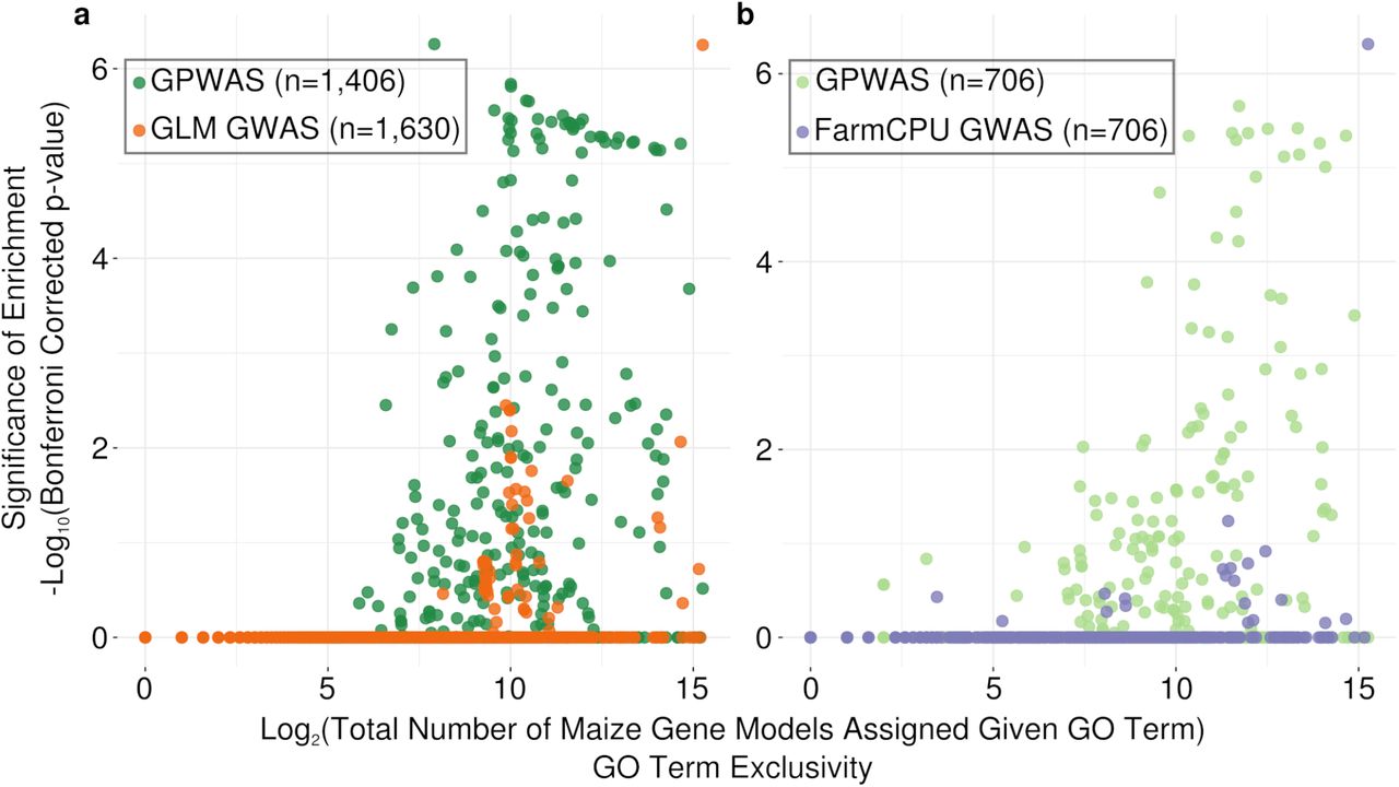
Perhaps one of the most striking features distinguishing the genes identified by GPWAS and GWAS was enrichment of functional annotation categories. A total 137 GO terms showed statistically significant (Bonferroni corrected p < 0.05) enrichment (119 terms) or purification (18 terms) among the 1,406 genes uniquely identified (relative to GLM GWAS) by GPWAS. In contrast only 15 GO terms (11 enriched and 4 purified) were identified in the corresponding set of 1,630 genes uniquely identified by GLM GWAS (Figure 3a, Supplemental Table S6). Consistent with theoretical models, genes annotated as involved in a wide range of terms related to development, response to stimuli, cell wall and cell membrane metabolism, hormone signalling, disease response, and transport were all over represented among genes associated with phenome-wide variation, while those associated with nucleotide metabolism, DNA replication, translation, and telomere organization were disproportionately unlikely to show such associations. Not only more GO terms were enriched in genes uniquely identified by the GPWAS model, but the p values of those enriched GO terms tends to be more significant (Figure 3a). To exclude the possibility that this result was due to differences in the quality of the annotations assigned to different populations of genes the quality and quantity of the annotations assigned to genes in different populations was examined. Noe single factor, including number of GO terms per gene and proportion of genes with no assigned GO term differed dramatically between these populations, although there were modest biases towards genes uniquely identified by GPWAS (Supplemental Table S6). Analysis using the 706 genes uniquely detected genes by FarmCPU GWAS found only a single significantly enriched GO term G0:0009987 ‘cellular process”, while, even when the number of uniquely GPWAS-identified genes was constrained to be identical to the number of uniquely identified FarmCPU GWAS genes, 67 GO terms still showed significant enrichment (58 terms) or purification (9 terms) (Figure 3b, Supplemental Table S6). No single obvious factor explained the difference in functional enrichment results between the genes uniquely identified by GWAS and GPWAS, but a number of factors including number of GO terms per gene and proportion of genes with no assigned GO term differed modestly (Supplemental Table S7). The median GO term assigned to a gene identified only by GPWAS was assigned to only 430 gene models in B73 RefGenv4, while the median GO term assigned to a gene identified only by GLM GWAS was assigned to 514 different gene models. Thus, even though genes uniquely identified by either GPWAS or GWAS were annotated with approximately equal numbers of GO terms per gene, the GO terms assigned to genes identified by GPWAS were somewhat more exclusive categories. However, the large differences in functional enrichment/purification observed are consistent with GPWAS identifying a far less random subset of annotated genes than sequential GWAS for each of the same traits.
Gomparison of GO enrichment/purification among genes uniquely identified as associated with phenotypic variation using different statistical approaches. Each circle is a single GO term in a single analysis. The position of each circle on the x axis indicates the total number of maize gene models which were assigned this GO term in the maize GAMER dataset45. The position of each circle on the y axis indicates the statistical significance of the enrichment or purification of this GO term in the given gene population relative to the background set of all annotated maize gene models. (a) Comparison of the patterns of GO term enrichment/purification among genes either either uniquely identified as associated with phenotypic variation by GLM GWAS analysis or uniquely identified as associated with phenotypic variation by GPWAS analysis. (b) As in panel A, but comparing genes uniquely identified as associated with phenotypic variation by FarmCPU analysis or uniquely identified as associated with phenotypic variation by GPWAS analysis. Only to706 genes uniquely identified by GPWAS with the strongest statistical signal were employed in panel B, to prevent any bias towards more significant p-values which would result from conducting the analysis with a larger population of genes for GPWAS than for FarmCPU.
Discussion
The GPWAS model selects an optimal combination of phenotypes to maximize explanatory power for the set of genetic variants present within a given gene. As described for Anther ear1, in some cases the phenotypes selected for the model are consistent with known gene function from in depth single gene studies. However, it is important to note two limitations in the interpretation of the specific traits incorporated into the models of individual genes. The first is that the incorporation of individual traits are not subject to false discovery control. Therefore, a gene correctly identified as showing statistically significant association with the trait dataset as a whole may still include one or more traits within its model with which it has no direct functional link. The second is that the stepwise regression procedure means that traits where variance truly is controlled in part by the target gene may be excluded if a second trait exists in the dataset which captures the same functional link46. Our present GPWAS model has several critical limitations. The first is that the statistical tests employed require a complete absence of missing data, hence the dependence on both genotypic as well as phenotypic imputation. Large scale trait datasets will almost always have at least a few missing data points, so it is only because advances in kinship based phenotypic imputation that the present study became viable33. The second is that our approach required binning individual genetic markers into groups associated with individual genes. This binning is likely to be imperfect, as regulatory regions of genes can be separated from coding sequence by tens of Kb in maize47, 48. Noncoding regulatory sequences, many distant from annotated genes, have been shown to explain approximately 40% of the total phenotypic variation in maize49. Finally, our present GPWAS algorithm and implementation is quite computationally expensive. Including the permutations required to establish effective false discovery rate estimates, we estimate the GPWAS analyses presented here required a total of approximately 6.9 years of CPU (Intel Xeon E5-2670 2.60GHz processor) time and was only possible with access to a high performance computing core facility and because the approach taken falls into the embarrassingly parallel class of computational problems.
To our knowledge the Panzea trait dataset for the Buckler-Goodman association panel presently represents one of only a handful of extremely trait dense datasets for a single population in the plant world. However, the rapid emergence of high throughput plant phenotyping technologies makes it likely that high dimensional trait datasets – where the number of measured phenotypes exceeds even the number of individuals in the population – will become much more common in the future27,28. Many high-throughput phenotyping technologies collect images, hyperspectral data cubes, or LIDAR point clouds from which many distinct plant traits can be scored for the same individual plants or plots. Thus, models which can integrate data from many traits scored in a single population will be an area of greater need going forward. While increasing the total number of phenotypes scored and included as potential predictors should increase the power and accuracy of GPWAS, if many highly correlated traits are included, the result can be issues with multicollinearity that make the statistical estimation and inference procedures we employed unstable. With the current statistical procedure, issues are likely to arise in cases where the number of input traits exceeds the number of individuals in the population. One common approach to reducing the total number of traits in a multiyear and/or multi-field site trial is to calculate best unbiased linear predictors (BLUPs) which provide a single value for a given trait in a given line across multiple environments50. However, this approach strips out information on trait plasticity across environments, which is often controls by distinct sets of genes from genes controlling variation in multi-environment trait means51 and is thus likely to bias downstream analysis away from a large class of genes involved in determining organismal phenotypes. In cases where the number of measured traits exceeds the number of environments, it would be advisable to employ alternative approaches to reduce the dimensionality of the trait dataset, whether an ad hoc approach such as selecting a subset of representative traits from highly correlated blocks, or dimensional reduction analyses such as principal component analysis or multidimensional scaling. Automatic application of variable selection and/or dimensional reduction in such scenarios could be incorporated into future GPWAS implementations. As always, the simple to propose but resource intensive to implement solution would be to augment the size of frequently employed association populations going forward.
Over the past three decades, without substantial discussion or debate, many in the scientific community have moved from a definition of genes that was based on organismal function, to one which is based on molecular features52–54. However, many analysis still contains the implicit assumption that genes annotated in the genome based on homology and/or expression evidence must play a role in determining organismal phenotypes. Absence of evidence for a role in determining phenotype is interpreted as a failure to find either the correct trait to measure or the correct environment in which to measure it. Here we have developed a new approach to identify genes with statistical links to a variation in a large set of diverse plant traits scored for a maize diversity panel across a diverse set of environments, and showed that it exhibits greater consistency with genes identified as controlling organismal phenotypes in an independent population than do genes identified using two conventional GWAS approaches. GPWAS was also found to provide a more favorable trade off between FDR and power than conventional trait-by-trait GWAS in simulations based on the same individuals and genotype calls described above and 100 phenotypes of varying heritability (Supplemental Figure S4). Using real world trait data, we found that genes with statistically significant links to phenotypic variation exhibit substantial differences in a number of characteristics from the overall population of annotated genes in the maize genome. They are more likely to be transcribed to significant levels, likely to be conserved at syntenic orthologous positions in the genomes of related species, dramatically less likely to exhibit presence absence variation across diverse maize inbreds, appear to be subjected to notably stronger purifying selection than the overall population of annotated genes, and are enriched in a wide range of functional annotations relative to the overall population of annotated genes. The distinct features of both genes identified as controlling organismal phenotypes by classical forward genetics and now by GPWAS indicate that it is unlikely all annotated genes in the maize genome do indeed contribute to organismal phenotypes. Improved approaches to distinguish genes which contribute to organismal phenotypes from those which do not will be critical to developing genotype-to-phenotype models going forward.
Methods
Genotype and Phenotype Sources, Filtering, and Imputation
Raw genotype calls in AGPv4 coordinates from resequencing of the maize 282 association panel30 were retrieved from PanZea. Missing genotypes were imputed using Beagle (version: 2018-06-10)55. Only biallelic SNPs with less than 80% missing points were input for imputation. After imputation, SNPs with MAF (Minor Allele Frequency) less than 0.05 or which were scored at heterozygous in more than 10% of samples were discarded. A phenotype file (traitMatrix_maize282NAM_v15-130212.txt) containing total of 285 traits, corresponding to 57 unique types of phenotypes scored in 1-16 environments was downloaded from PanZea. A set of 277 accessions with identical names in the HapMap3 data release and the PanZea trait data were employed for all downstream analyses.
Maize gene regions were extracted from AGPv4.39 downloaded from Ensembl. SNPs were clustered based on R2 > 0.8 and only one randomly selected SNP per cluster was retained. If the number of SNPs after collapsing highly correlated clusters exceeded 138 (50% of the number of inbreds scored), a random subsample of 138 SNPs was employed for downstream analyses. Identical final SNP sets were employed for GWAS and GPWAS analyses.
Of the 285 initial trait datasets, 25 were removed because the data file contained a recorded trait value for only a single individual among the 277 maize inbreds genotyped, leaving a total of 260 trait datasets. Missing phenotypes were imputed based on a kinship matrix calculated from 1.24 million SNPs calculated in GEMMA18 and using a Bayesian multiple-phenotype mixed model33. Accuracy of phenotypic imputation was assessed independently for each trait with sufficient number of real observations to evaluation using ten iterations of masking 1% of available records for each trait and comparing imputed and masked values for each trait.
GPWAS Analysis
We propose a model selection approach to adaptively choose the most significant phenotypes associated with each gene. Given a gene, we consider all the SNPs as the multi-responses, and include the first three PC scores for this gene. Let αin and αout be the criterion thresholds for the p-values of the phenotypes. If a phenotype with p-value smaller than αin, we consider it as potentially significant and should be added into the regression model. Whereas, if the p-value of an existing phenotype in the model is larger than αout, we consider it as insignificant and exclude it from the model. As a default, we choose αin = αout = 0.01 for each gene.
The stepwise selection procedure is as follows:
Start with the multi-response model with all the SNPs as responses and the first three PC scores as covariate. Search for the the most significant phenotype across all the phenotype measurements. Include this phenotype into the model if its p-value is below αin. Otherwise, declare no phenotype is significant for this gene.
For the ℓth step, add each one of the remaining phenotypes into the existing model with the covariates that have already been selected, and calculate its p-value. This p-value measures the effect of this phenotype on the responses given all the selected phenotypes from the previous steps.
Find the remaining phenotype with the minimum p-value. Include this phenotype into the model if its p-value is below αin. Otherwise, declare no new add in.
The newly added covariate may be correlated with the existing covariates in the model. This may change their corresponding p-values. Fit all the selected phenotypes jointly in the model and drop the phenotype with the largest p-value that is greater than the cutoff value αout.
Repeat steps (2), (3) and (4) until no phenotypes can be added or removed from the model. This is considered as the final model for the targeted gene.
The final model can be represented as:

Here, there are vi selected phenotypes for the ith gene, where vi ≤ 260. The selected phenotypes {Phek,(j)} are a subset of the collection of the all the phenotypes {Phek, 1, Phek,2,…, Phek,260}, where τi,j is the corresponding coefficients for selected phenotypes for the ith gene and the phenotype effects τij from the stepwise selection model incorporates the dependence among phenotypes. First three PC scores PC1, PC2 and PC3 were always included in the model with effect size of βi1, βi2 and βi3. Total phenotypes was iteratively selected for 35 times for each scanned gene. All the unselected phenotypes were considered as insignificant for a particular gene. The p-value of each gene was determined by partial F test through comparing the final model containing both the first three PCs and the selected phenotypes with the initial model containing only the PCs.
FDR cut offs were based on the results from 20 permutation analysis where the values for each trait where independently shuffled among the 277 genotyped individuals and the entire GPWAS pipeline rerun for all genes. The code implementing the above analyses in R and associated documentation has been published as the “GPWAS” and is avaliable from the following link: https://github.com/shanwai1234/GPWAS. Selected significant GPWAS genes with incorporated phenotypes were listed in Supplemental Table S8.
GWAS Analysis
GLM GWAS analyses were conducted using the algorithm first defined by Price and coworkers56 and FarmCPU GWAS with the algrothm defined by Liu and colleagues57. Both algorithms were run using the R-based software MVP (A Memory-efficient, Visualization-enhanced, and Parallel-accelerated Tool For Genome-Wide Association Study) (https://github.com/XiaoleiLiuBio/MVP). Both analysis methods were run using maxLoop = 10 and the variance component method method.bin = “Fast-LMM”58. A subset of 1.24 million SNPs distributed across both intragenic and intergenic regions on all 10 chromosomes was used to perform principle component analysis (PCA). For analysis of genes on each chromosome, a separate PCA was conducted using markers solely from the other 9 chromosomes to reduce the endogenous correlations between genes and principle components59, and the first three PCs were included in each GWAS analysis. For comparison to GPWAS results, each gene was assigned the p-value of the single most significant SNP among all the SNPs assigned to that gene in the GPWAS model.
Nested Association Mapping Comparison
Published associations identified for 41 phenotypes scored across 5,000 maize recombinant inbred lines were retrieved from Panzea (http://cbsusrv04.tc.cornell.edu/users/panzea/download.aspx?filegroupid=14)31. Following the thresholding proposed in that paper a SNP and CNV (copy number variant) hits with a resample model inclusion probability ≥ 0.05 which were either within the longest annotated transcript for each gene AGPv2.16 or within 15kb upstream or downstream from the annotated transcription start and stop sites were assigned to that gene. Gene models were converted from B73 RefGenV2 to B73 Re-fGenV4 using a conversion list published on MaizeGDB (https://www.maizegdb.org/search/gene/download_gene_xrefs.php?relative=v4).
Gene Expression Analysis
Raw reads from the a published maize expression atlas generated for the inbred B73 were downloaded from the NCBI Sequence Read Archive PRJNA17168441. Reads were trimmed using Trimmomatic-0.38 with default setting parameters60. Trimmed reads were aligned to the maize B73 RefGenv4 reference genome using GSNAP version 2018-03-2561. Alignment results were converted to sorted BAM file format using Samtools 1.662 and Fragments Per Kilobase of transcript per Million mapped reads (FPKM) where calculated for each gene in the AGPv4.39 maize gene models in each sample using Cufflinks v2.263. Only annotated genes located on 10 maize pseudomolecules were used for downstream analyses and the visualization of FPKM distribution.
Ka/Ks Calculations
For each gene listed in a public syntenic gene list,64, the coding sequence for the single longest transcript per locus was downloaded from Ensembl Plants and aligned to the single longest transcript of genes annotated as syntenic orthologs in Sorghum bicolor in v3.165 and Setaria italica v2.266 were retrieved from Phytozome v12.0 using a codon based alignment as described previously67. The calculation of the ratio of the number of nonsynonymous substitutions per non-synonymous site (Ka) to the number of synonymous substitutions per synonymous site (Ks) was automated using in-house constructed software pipeline posted to github (https://github.com/shanwai1234/Grass-KaKs). Genes with synonymous substitution rate less than 0.05 were excluded from the analyses as the extremely small number of synonymous substitutions tended to produce quite extreme Ka/Ks ratios and genes with multiple tandem duplicates were also excluded from Ka/Ks calculations. Calculated Ka/Ks ratios of maize genes were provided in Supplemental Table S9.
Presence/Absence Variation (PAV) Analysis
PAV data was downloaded from a published data file42. Following the thresholding proposed in that paper, a gene was considered to exhibit presence absence variance if at least one inbred line with coverage less than 0.2.
Gene Ontology Enrichment Analysis
GO analysis was conducted using goatools68 and using a set of GO annotations generated for B73 in RefGen_V4 using maize-GAMER45. Fisher test was conducted using SciPy stats package fisher_exact.
Power and FDR evaluation of GPWAS and GWAS using simulated data
SNP calls for the entire set of 1,210 individuals included in Maize HapMap3 were retrieved from Panzea30, filtered, imputed, and assigned to genes as described above resulting in 1,648,398 SNPs assigned to annotated gene body regions in B73 RefGenV4. 2,000 randomly selected genes associated with 30,547 SNP markers were employed for downstream simulations. In each simulation, 100 genes (5%) were selected as causal genes. For each causal gene in each simulation, a causal SNP was selected for simulating phenotypic effects. A total of 100 phenotypes were simulated in each permutation of the analysis, with 10 traits simulated with heritability of 0.7, 30 traits simulated with heritability of 0.5 and 60 traits simulated with heritability of 0.3. Effect sizes for each SNP for each phenotype in each permutation were drawn from a normal distribution centered on zero using the additive model in GCTA (version 1.91.6)69.
The resulting simulated trait data and genuine genotype calls were analyzed using GLM GWAS, FarmCPU GWAS, and GPWAS as described above with the exception of calculating population structure principle components using a sample (1% or 157,748 SNPs) of the total SNPs remaining after filtering, rather than only the subset of SNPs assigned to the 2,000 randomly selected genes included in this analysis. For each analysis, the set of 2,000 genes was ranked from most to least statistically significant based on the significance of the single most significantly associated SNP (for GLM and FarmCPU GWAS) or the significance of the overall model fit relative to a population structure only model (for GPWAS). Power evaluation for GPWAS was defined as the number of true positive genes to the total number of causal genes and FDR was defined as the number of false positive genes to the total number of positive genes. Power and FDR were calculated in a step size of five genes from 5 total positive genes to 500 (ie {5,10,…,450,500}).
Acknowledgements
This work is supported by the Quantitative Life Sciences Initiative at the University of Nebraska-Lincoln, which receives support from a University of Nebraska Program of Excellence and by the National Science Foundation Awards MCB-1838307 and OIA-1826781 to JCS. The authors thank Andy Dahl advice and instruction in the use of phenotype imputation, Zheng Xu and Wenlong Ren for consultation on the design of the association study, and the PanZea project (http://www.panzea.org) for gathering the phenotypic and genotypic data employed in this study. This work was completed utilizing the Holland Computing Center of the University of Nebraska, which receives support from the Nebraska Research Initiative.
References


