

Abstract
Electroencephalographic (EEG) source imaging depends upon sophisticated signal processing algorithms for data cleaning, source separation, and localization. Typically, these problems are addressed by independent heuristics, limiting the use of EEG images on a variety of applications. Here, we propose a unifying parametric empirical Bayes framework in which these dissimilar problems can be solved using a single algorithm (PEB+). We use sparsity constraints to adaptively segregate brain sources into maximally independent components with known anatomical support, while minimally overlapping artifactual activity. Of theoretical relevance, we demonstrate the connections between Infomax ICA and our framework. On real data, we show that PEB+ outperforms Infomax for source separation on short time-scales and, unlike the popular ASR algorithm, it can reduce artifacts without significantly distorting clean epochs. Finally, we analyze mobile brain/body imaging data to characterize the brain dynamics supporting heading computation during full-body rotations, replicating the main findings of previous experimental literature.
Introduction
The electroencephalogram (EEG) is a noninvasive functional brain imaging modality that allows the study of brain electrical activity with excellent temporal resolution. Compared to other noninvasive imaging modalities such as fMRI, PET, SPECT, and MEG, EEG acquisition can be mobile and more affordable [Mcdowell et al., 2013, Mehta and Parasuraman, 2013], allowing the widespread study of human cognition and behavior under more ecologically valid experimental conditions [Makeig et al., 2009]. Imaging cognitive processes while participants engage naturally with their environment (natural cognition in action [Gramann et al., 2014]) has potential for developing a new generation of applications in brain-computer interfaces (BCI), mental health, rehabilitation, and neuroergonomics [Mishra and Gazzaley, 2014, Jungnickel and Gramann, 2016, Wagner et al., 2016]. However, despite impressive methodological advances in the estimation of the electrical activity of the cortex from EEG voltages recorded on the scalp, a number of practical and theoretical issues remain unsolved.
Imaging EEG source activity (also known as electromagnetic source imaging or ESI) is challenging for several reasons. First, since many configurations of currents in the brain can elicit the same EEG scalp topography [Michel and Murray, 2012], it entails solving an ill-posed inverse problem [Lopes da Silva, 2013]. Second, the EEG signal is often contaminated by artifacts of non-brain origin such as electrooculographic (EOG) and electromyographic (EMG) activity that need to be identified and removed. Third, there is evidence that large-scale brain responses measured by EEG are generated by underlying cortical dynamics that evolve over time and can exhibit nonlinear features [Breakspear, 2017, Khambhati et al., 2018], thereby rendering the simplifying assumptions of linearity and stationarity used by most inverse methods hard to justify. These problems are usually addressed separately using a variety of heuristics, making it difficult to systematize a methodology for obtaining biologically plausible EEG source estimates in the presence of artifacts and nonlinear and nonstationary dynamics. The objective of this paper is to develop a unifying Bayesian framework in which these, apparently dissimilar, problems can be understood and solved in a principled manner using a single algorithm.
To cope with the ill-posed nature of the inverse problem and ensure functional images with biological relevance, several inverse algorithms have been proposed that seek to estimate EEG sources subject to neurophysiologically reasonable spatial [Haufe et al., 2011, Friston et al., 2008, Trujillo-Barreto et al., 2004, Pascual-Marqui et al., 2002, Baillet et al., 2001], spatiotemporal [Martínez-Vargas et al., 2015, Valdés--Sosa et al., 2009, Trujillo-Barreto et al., 2008], and frequency-domain [Gramfort et al., 2013] constraints, just to mention a few examples. These approaches can work relatively well when the EEG samples are corrupted by Gaussian noise and the signal to noise ratio (SNR) is high. In practice, however, raw EEG data are affected by many other types of noise such as interference from the 50/60 Hz AC line, pseudorandom muscle activity, and mechanically induced artifacts, among others. Thus, before source estimation, non-Gaussian artifacts need to be removed from the data.
There is a plethora of methods for dealing with artifacts corrupting the EEG signal [Mannan et al., 2018, Islam et al., 2016]. Popular approaches used in real-time BCI applications are based on adaptive noise cancellation [Kilicarslan et al., 2016] or Artifact Subspace Removal (ASR) [Mullen et al., 2015] algorithms. The former has the inconvenience that an additional channel recording purely artifactual activity (i.e., EOG or EMG activity not admixed with EEG) needs to be provided, while the latter rests on the assumption that the statistics of data and artifacts stay the same after an initial calibration phase. In studies where the data can be analyzed offline, artifactual components can be largely removed using Independent Component Analysis (ICA) [Jung et al., 2000]. ICA-based cleaning, however, has the drawback that non-brain components need to be identified for removal, which is usually done manually based on the practitioner’s experience.
ICA is a special case of blind source separation (BSS) method [Cichocki and Amari, 2002] that can be used to linearly decompose EEG data into components that are maximally statistically independent. ICA has been used to analyze event-related potentials (ERP) under the assumptions that during the task 1) the decomposition is stationary and 2) that brain components can be modeled as a predefined number of dipolar point processes with fixed spatial location and orientation [Makeig and Onton, 2011]. The stationarity assumption can be relaxed using a mixture of ICA models [Palmer et al., 2011] while the selection of brain scalp projections is typically done either manually or automatically based on the residual variance afforded by a dipole fitting algorithm. The practical use of ICA has been limited by its computational cost and the need for user intervention. Only recently, a real-time recursive ICA algorithm has been proposed [Hsu et al., 2016], as well as a number of automatic methods for minimizing the subjectivity of manual component selection [Tamburro et al., 2018, Pion-Tonachini et al., 2017, Radüntz et al., 2017]. Despite these advances, turning ICA into a brain imaging modality requires that after source separation, we solve the inverse problem of localizing the set of identified brain components into the cortical space.
One way of estimating EEG sources subject to multiple assumptions (constraints) in a principled manner is to use the framework of parametric empirical Bayes (PEB) [Morris, 1983, Casella, 1985]. In this framework, constraints are used to furnish prior probability density functions (pdfs). Empirical Bayes methods use data to infer the parameters controlling the priors (hyperparameters), such that those assumptions that are not supported by the data can be automatically discarded without user intervention. Here we use priors to “encourage" source images to belong to a functional space with biological relevance, but the exact form of those priors is determined by the data (empirically). In the context of sparsity-inducing priors, PEB is sometimes referred to as Sparse Bayesian Learning (SBL) [Tipping, 2001]. The PEB framework has been applied extensively to brain imaging for inverting hierarchical models of fMRI and PET [Friston et al., 2002] as well as EEG responses [Henson et al., 2011, Friston et al., 2008].
In this paper, within the PEB framework, we propose a probabilistic generative model (PGM) of how the raw EEG time series arises from the superposition of the brain and non-brain (artifact) source activity. We use an anatomical brain atlas to parameterize the source prior such that we induce sparsity in the number of cortical regions active at any given time (this is known in the SBL literature as block-sparsity [Zhang and Rao, 2013]). Then, our model can be inverted using an efficient block SBL algorithm recently proposed by Ojeda et al. [2018]. Henceforth, we refer to this new approach as PEB+ (PEB with the addition of artifact modeling). Our main contribution is that, by explicitly modeling non-brain sources within the PEB framework, we can unify three of the most common problems in EEG analysis: data cleaning, source separation, and source imaging. In addition, we show that the PEB+ algorithm has online adaptation, thereby allowing it to capture transient brain dynamics. On the theoretical side, we point out the connections between distributed source imaging and ICA, two popular approaches that are often perceived to be at odds with one another.
The rest of the paper is organized into two main sections concerned with methods and results respectively. Methods: In Section 2.1 we propose the augmented PGM of the EEG taking into account the contribution of artifact sources and motivate all our modeling assumptions. In Section 2.2 we outline the model inversion algorithm. In Sections 2.3–2.3.1 we point out the connections between PEB+ and ICA. Results: In Section 3.1 we explain how to construct an empirical dictionary of artifact scalp projections. In Sections 3.2, 3.3, and 3.4 we investigate the respective source imaging, separation, and data cleaning capabilities of the PEB+ algorithm.
Throughout this paper we use lowercase and uppercase bold characters and symbols to denote column-vectors and matrices respectively,  is an estimate of the parameter vector a, and IN is a N × N identity matrix.
Methods
It has been shown that popular source estimation algorithms used in ESI such as weighted minimum l2-norm [Baillet et al., 2001], FOCUSS [Cotter et al., 2005, Gorodnitsky and Rao, 1997], minimum current estimation [Huang et al., 2006], sLORETA [Pascual-Marqui et al., 2002], beamforming [Van Veen et al., 1997], variational Bayes [Friston et al., 2008], and others can be expressed in a unifying Bayesian framework [Wipf and Nagarajan, 2009]. We extend this framework by explicitly modeling non-brain artifact sources.
2.1 Augmented probabilistic generative model
In source imaging, the neural activity is often referred to as the primary current density (PCD) [Baillet et al., 2001] and it is defined on a grid of known cortical locations (the source space). Typically, a vector of Ny EEG measurements at sample k,  , relates to Ng PCD values,
  , through the following linear equation [Dale and Sereno, 1993],
 where
where  represents the measurement noise vector. The PCD is projected to the sensor space through the lead field matrix
 where each column li denotes the scalp projection of the ith unitary current dipole with fixed orientation within the source space. When dipole orientations are considered, then
  and we determine a source vector
  . The lead field matrix is usually precomputed for a given electrical model of the head derived from a subject-specific MRI [Hallez et al., 2007]. Alternatively, if an individual MRI is not available, an approximated lead field matrix obtained from a high-resolution template can be used [Huang et al., 2016]. Then, the inverse problem of the EEG can be stated as the estimation of a source configuration ĝk that is likely to produce the scalp topography yk.
In the generative model presented above, the noise term ek is assumed to be Gaussian and spatially uncorrelated with variance λ. This simplification is acceptable as long as EEG topographies are not af-fected by non-Gaussian pseudo-random artifacts gen-erated by eye blinks, lateral eye movements, facial and neck muscle activity, body movement, among oth-ers. Therefore, before source estimation, EEG data are usually heavily preprocessed and cleaned [Bigdely-Shamlo et al., 2015]. Since artifacts contribute linearly to the sensors, ideally, one would like to characterize their scalp projections to describe more accurately the signal acquisition. To this end, we propose the following generalization of Eq (1),
 where
where  is a vector of Nν artifact sources and
  is a dictionary of artifact scalp projections (see Fig 1).

Proposed augmented generative model of the EEG. The model postulates that the EEG scalp topography yk arises from the linear superposition of brain gi,k and artifact νj,k components weighted by their respective scalp projections li and aj, corrupted by spatially uncorrelated Gaussian noise ek.
Although the entries of A that correspond to muscle activity may be obtained based on a detailed electromechanical model of the body [Böl et al., 2011], in most studies this approach may not be feasible due to computational and budgetary constraints. Janani et al. [2017] modelled A by expanding the lead field matrix to account for the contribution of putative scalp sources, which were assumed to be the generators of EMG activity. They used sLORETA to estimate brain and scalp sources simultaneously. Although this approach was shown to be as effective as ICA-based artifact removal, it was suggested by the authors that the use of the non-sparse solver sLORETA may lead to unrealistic configurations of brain and non-brain sources. Similarly, Fujiwara et al. [2009] augmented the magnetic lead field matrix to model the scalp contribution of two current dipoles located behind the eyes and used a Bayesian approach, that has similarities with ours, to estimate brain and eye source activity from MEG data. Although success-ful for removing EOG activity, in their formulation, Fujiwara et al. [2009] ignored other types of artifacts that are harder to model such as those produced by muscular activity.
In this paper, we take an empirical view inspired by the success of ICA-based artifact removal approaches. We propose constructing the dictionary A using a set of stereotypical artifact scalp projections such as those obtained from applying ICA to a database of EEG recordings [Bigdely-Shamlo et al., 2013a]. We then rewrite Eq (2) in a compact manner as follows,
 where the gain matrix is now H ≜ [L,A] and
 is the augmented vectorT of hidden (latent) brain and artifact sources (see Fig 1).
Note that, structurally, the standard generative model in Eq (1) and the augmented one in Eq (3) are identical. They differ however in that in Eq (3) we are explicitly modeling the instantaneous spatial contribution of non-brain sources to the scalp topography yk. Therefore, we may be able to dispense with computationally expensive preprocessing data cleaning procedures. The assumption of Gaussian measurement noise yields the following likelihood function,

Since Eq (3) does not have a unique solution, to obtain approximated source maps with biological interpretation we introduce constraints. One way of incorporating constraints in a principled manner is to express them in the form of the prior pdf of the sources p(xk). Since the neural generators of the EEG are assumed to be the electrical currents produced by distributed neural masses that become locally synchronized in space and time [Nunez and Srinivasan, 2006], here we chose a parameterized prior p(xk) that induces source maps to be globally sparse (seeking to explain the observed scalp topography by a few spots of cortical activity) and locally correlated (so that we obtain spatially smooth maps as opposed to maps formed by scattered isolated sources). Artifactual sources, on the other hand, can be assumed to be uncorrelated from one another. We use a Gaussian prior to express these modeling assumptions as follows,
 where the covariance matrix Σx has a block diagonal structure [Zhang and Rao, 2013] defined as

In Eq (6), the brain source prior covariance is defined as
 and
and  is the covariance of artifact sources. The matrices
  encode the intra-group brain source covariances and are precomputed based on source distance respecting the local folding of the cortex as described in [Ojeda et al., 2018].
  denotes a nonnegative scale vector that encodes the sparsity profile of the group of sources. Here we define NROI = 148 groups based on anatomical regions of interest (ROI) obtained from the Destrieux cortical atlas [Destrieux et al., 2010]. We note that although other atlases could be used within the framework outlined in this section (e.g. the popular Desikan-Killiany 68-ROI cortical atlas [Desikan et al., 2006]), the discussion of issues pertaining to the selection of an optimal cortical parcellation is beyond the scope of this paper.
Next, let model  be the set of hyperparameters that encode the generative model proposed above. We use the Bayes theorem to express the posterior pdf of the sources given the data and model as,

Note that  and
and 
 because the likelihood and priors are independent of γ and λ respectively. The density function
  is known as the model evidence [MacKay, 2008a] and, as we will show latter, its optimization allows us to reshape our modeling assumptions in a data-driven manner.
The model evidence is the normalization constant of the posterior in Eq (8), therefore it can be ignored while searching for the maximum a posteriori (MAP) source estimate X̂k = XMAP, which we find as the mode of the numerator of Eq (8) conditioned on  ,
,

We readily determine the functional form of the posterior as  , with the following conditional mean and covariance [Wipf and Nagarajan, 2009],
 where the model data covariance is given by the following expression,

In case that we need to obtain the cleaned EEG signal  , e.g. for visualization or scalp ERP analysis, we subtract the artifact signal from the data as follows
 where
where  is a spatial filtering operator and
  is obtained (if needed) by selecting the last Nν elements of the vector x̂k. Likewise, the estimated PCD vector ĝk can be obtained by selecting the first Ng elements of x̂k or using the formula
 and the source activity specific to the the ith ROI can be obtained using the formula

Further analysis of the source time series (e.g. ERP and connectivity analysis) can be done by averaging the source activity obtained in Eq (14) within ROIs,
 where ROIi ⊂ {1, …, Ng} is the subset of indices that belong to the ith ROI.
2.2 Model learning
The source estimates and cleaned data can be obtained analytically by evaluating the formulas given in Eq (10)–(13). These formulas, however, are model dependent because they depend on the specific values of the hyperparameters λ and γ. In this section we outline the algorithm for learning those.
To evaluate Eq (10) conditioned on the optimal model estimate we maximize the posterior density,
 Where
Where  and
and  is a hyperprior. To determine the evidence described in Eq (8) we need to marginalize out the sources,
 which for a linear Gaussian model like ours, is readily expressed as [Barber, 2012],

Next, we need to specify the hyperprior  . Assuming that λ and γi are independent yields the factorization
  . Since
  contains only scale hyperparameters, a popular choice is to assume Gamma hyperpriors on a log-scale of λ−1 and
  [Tipping, 2001]. When the scale and shape parameters of the Gamma tend to zero the hyperpriors become flat (noninformative), in which case the optimization of the model posterior density depends only on the model evidence. This choice of hyperprior has the effect of assigning a high probability to low values of γi, which tends to shrink the irrelevant components of xk to zero, leading to a sparsifying behavior know as Automatic Relevance Determination (ARD) [Neal, 1996, MacKay, 1992].
To obtain robust hyperparameter estimates in an online fashion, we use a block of consecutive measurements Y = [yk, …, yk+N] as opposed to a single data point yk. Here we assume that the parameters characterizing the generative model vary at a slower rate compared to the brain and artifact dynamics producing the measurements. In other words, sources producing a given data block Y are not expected to go silent from one sample to the next. This assumption can be further motivated by the fact that the EEG can be temporally segmented into a sequence of discrete quasi-stable microstates, each of which consisting of a scalp configuration lasting for approximately 80 to 120 milliseconds before transitioning to a different microstate [Khanna et al., 2015, Van De Ville et al., 2010, Koenig et al., 2002]. With this in mind, we ignore short-term correlations within a Y block (iid assumption) and approximate the evidence of the ensemble as,
 where N is set so that we deal with consecutive blocks of approximately 40 milliseconds in a way that we don’t miss microstates.
The maximization of the model block evidence is equivalent to minimizing the so-called type-II Maximum Likelihood (ML-II) cost function [Barber, 2012], which is obtained by applying −2log(·) to Eq (19),
 where Cy = N−1YYT is the empirical data covariance. Note that the data should be zero-mean, which can be achieved with a high-pass filtering stage during preprocessing. Eq (20) embodies a tradeoff between model complexity and accuracy. Geometrically, the complexity term represents the volume of an ellipsoid defined by Σy. In particular, as the axes of the ellipsoid shrink due to the pruning of irrelevant sources, the volume is reduced. The second term measures model accuracy; i.e., how similar are the empirical and analytic covariances Cy and Σy. We update the model on every block by solving the following optimization problem

Eq (21) can be optimized very efficiently following a two-stage approach proposed by Ojeda et al. [2018]. In the first stage we learn a coarse-grained non-sparse model by solving the constrained optimization problem:

In the second stage we fix λ to the value  and, starting from the value
  , we learn the sparse model by solving the optimization problem:

An intuitive explanation for why the optimization of the ML-II cost function in Eq(20) yields sparse sources can be found in [Tipping and Faul, 2003]. We point the reader interested in the details of the two-stage algorithm outlined in this section to [Ojeda et al., 2018] while the MATLAB code and examples can be freely downloaded from the Distributed Source Imaging (DSI) toolbox repository2.
2.3 Connections between PEB+ and ICA
In the analysis presented above, the matrix H is prespecified. In this section, we analyze the generative model of Eq. (3) from the ICA viewpoint. ICA is a blind source separation method that seeks to estimate the source time series (often called activations in the ICA literature) xk from the data time series yk without knowing the gain (mixing) matrix H. In ICA, we assume that the latent sources are instantaneously independent, which yields the following prior distribution

To simplify the exposition, we assume the same number of sensors and sources, Ny = Nx, and the interested reader can find the case Ny < Nx in [Le et al., 2011, Lewicki and Sejnowski, 1998]. From these premises, the objective of the algorithm is to learn the unmixing matrix H−1 such that we can estimate the sources with  . The unmixing matrix
  can be learned up to a permutation and rescaling factor, which has the inconvenience that the order of the learned components can change depending on the starting point of the algorithm and data quality. We can use a data block Y to write the likelihood function
 under the assumption of independent data collection. However, we should point out that in ICA, Y is usually a data block longer than the one considered in Section 2.2, thus the iid data assumption is harder to justify. To alleviate this situation the data are usually whitened during preprocessing. We can obtain each factor in Eq (25) by integrating out the sources as follows

As noted by MacKay [2008b], assuming that the data are collected in the noiseless limit, λ → 0, transforms the Gaussian likelihood p(yk|xk, H, λ) into a Dirac delta function, in which case Eq (26) leads to the Infomax algorithm of Bell and Sejnowski [1995]. The learning algorithm essentially consists in finding the gradient of the log likelihood, logp(Y|H, λ), with respect to H and updating H on every iteration such that the probability of the data increases. As pointed out by Comon [1994], the ICA model is uniquely identifiable only if at most one component of xk is Gaussian. Therefore, the prior densities pi(xi,k) are usually assumed to exhibit heavier tails than the Gaussian and, in particular, the prior pi(xi,k) ∝ cosh−1xi,k yields the popular ICA contrast function tanh(H−1yk). Note that this prior is not motivated by a biological consideration but by a mathematical necessity.
It is remarkable that ICA can learn columns of  that are consistent with bipolar (single or bilaterally symmetric) cortical current source scalp projections without using any anatomical or biophysical constraint whatsoever [Makeig et al., 1997]. Onton et al. [2006] have shown that other columns may correspond to different stereotypical artifact scalp projections as well as a set of residual scalp maps that are difficult to explain from a biological standpoint. Delorme et al. [2012] have shown that the best ICA algorithms can identify approximately 30% of dipolar brain components (approximately 21 brain components out of 71 possible in a 71-channel montage). Although ICA has proven to be a useful technique for the study of brain dynamics [Makeig and Onton, 2011], we must wonder if its performance can be improved, perhaps by making BSS of EEG data less “blind”. In other words, if we know a priori what kind of source activity we are looking for (dipolar cortical activity, EOG and EMG artifacts and so on), why limit ourselves to a purely blind decomposition?
In this paper, we advocate the use of as much information as we can to help solve the ill-posed inverse problem. In that sense, the use of a prespecified lead field matrix in the generative model of the EEG forces inverse algorithms to explain the data in terms of dipolar sources, because the lead field is precisely an overcomplete dictionary of dipolar projections of every possible source there is in a discretized model of the cortex. It has been shown that source estimation can greatly benefit from the use of geometrically realistic subject-specific [Cuspineda et al., 2009] or, alternatively, population-based approximated lead fields matrices [Valdés-Hernández et al., 2009]. Furthermore, augmenting the lead field dictionary with a set of stereotypical artifact projections, as proposed in Section 2.1, furnishes a more realistic generative model of the EEG in a way that renders blind decomposition unnecessary or at least suboptimal for brain imaging.
2.3.1 Independent components through PEB+
Since the source activity measured in the EEG is mixed by the volume conduction effect, ideally, we would like the PEB+ framework to exhibit the ICA property of yielding maximally independent (demixed) source time series. In this section we show that this is indeed the case. We start by rewriting the biologically motivated source prior of Eq (5) as
 where each factor is a Gaussian pdf and i indexes a group of sources or an artifact component. To write Eq (27) as the ICA prior in Eq (24) we need to integrate out the hyperparameter γi from each factor as follows:
 which, given our choice of hyperprior on γi, renders each marginalized prior pi(xi,k) a heavy-tailed Student t-distribution [Tipping, 2001]. We note that in our development we take the route of optimizing the γi hyperparameters rather than integrating them out because the former approach yields a simpler algorithm and tends to produce more accurate results in ill-posed inverse problems [MacKay, 1996]. Moreover, the optimization of γi allows for automatic removal of irrelevant brain and artifact components that are not supported by the data, thereby eliminating the subjectivity implicit in manual component selection. Assuming the prior in Eq (27), the ICA data likelihood of Eq (25) becomes exactly the evidence of Eq (19), with the difference that in the PEB+ algorithm the H matrix is known and the evidence is optimized on small blocks of data, which gives our algorithm the ability to run in an online manner and to capture transient brain dynamics.
We summarize the advantages of using the PEB+ framework over ICA for source separation and imaging of EEG data as follows:
It deals gracefully with the overcomplete case (Ny « Nx) by finding the MAP source estimator, which always exist even in the presence of rank-deficient data, e.g. after removing the common average reference.
It deals with the redundancy in brain responses by inducing independence over groups of sources.
The use of the ARD prior allows for the automatic selection of components in a datadriven manner, thereby eliminating the subjectivity of selecting components based on practitioner’s experience.
It can adapt to non-stationary dynamics by updating the model on smaller blocks of data.
It can be used in online applications by leveraging fast evidence optimization algorithms.
Artifact removal, source separation, and imaging can be obtained simultaneously as a consequence of optimizing the evidence of a biologically informed generative model.
It facilitates subject-level analysis because we estimate the same number of cortical source activations per subject, each of which has known anatomical support. This eliminates the complications of clustering ICs and dealing with missing components [Bigdely-Shamlo et al., 2013b] while allowing the use of more straightforward and widespread statistical parametric mapping techniques [Penny et al., 2007].
Results
3.1 Construction of artifact projection dictionary A
The PEB framework has been validated extensively on simulated and real data elsewhere [Ojeda et al., 2018, Zhang and Rao, 2013, Henson et al., 2011, Friston et al., 2008]. In this section, we study the effects of modeling artifactual sources in the quality of the model inversion. We also discuss source separation through PEB+, as well as its use for data cleaning. Then in Section 3.5 we show an application of PEB+ to the study of heading computation during full-body rotations in the context of a mobile brain/body imaging (MoBI) experiment.
To characterize artifactual ICs we used data from two different studies made public under the umbrella of the BNCI Horizon 2020 project3 [Brunner et al., 2015]. Since in the next two sections we investigate different features of the PEB+ algorithm rather than the biological interpretation of its results, we don’t dwell into the details of the experimental paradigms used in each study, and we direct the interested reader to the respective publications referenced below.
3.3.1 Data set 1: Error related potentials
The first study, 013-2015, provided EEG data from 6 subjects (2 independent sessions per subject and 10 blocks per session) collected by Chavarriaga and del R. Millán [2010] using an experimental protocol designed to study error potentials during a BCI task. EEG samples were acquired at a rate of 512 Hz using a Biosemi ActiveTwo system and a 64-channels montage placed according to the extended 10/20 system.
3.1.2 Data set 2: Covert shifts of attention
The second data set, 005-2015, provided EEG and EOG data from 8 subjects collected by Treder et al. [2011] using an experimental protocol designed to study the EEG correlates of shifts in attention. The EEG was recorded using a Brain Products actiCAP system, digitized at a sampling rate of 1000 Hz. The montage employed had 64 channels placed according to the 10/10 system referenced to the nose. In addition, an EOG channel (labeled as EOGvu) was placed below the right eye. To measure vertical and horizontal eye movements, from the total of 64 EEG channels, two were converted into bipolar EOG channels by referencing Fp2 against EOGvu, and F10 against F9, thereby yielding a final montage of 62 EEG channels.
3.1.3 Data preprocessing and IC scalp maps clustering
After transforming each data file to the .set format, both studies were processed using the same pipeline written in MATLAB (R2017b The MathWorks, Inc., USA) using the EEGLAB toolbox [Delorme et al., 2011]. The pipeline consisted of a 0.5 Hz high-pass forward-backward FIR filter and re-referencing to the common average, followed by the Infomax ICA decomposition of the continuous data. We pooled all the preprocessed data sets and randomly assigned them to one of two groups: 80 % to the training set and 20 % to the test set. The training set was used to construct the artifact dictionary and the test set was used to evaluate the performance of the PEB+ algorithm.
To construct an artifact dictionary from a heterogeneous EEG database, we need to represent each independent scalp map into a common (co-registered) channel space. To that end, we used the coordinates of the common channels between the montages used in the two studies described above to estimate a linear transformation from the 62-channel space to the 64-channel one. After co-registration, we pooled both studies in the training set resulting in a matrix of 64 channels by 6774 independent scalp maps (101 sessions and blocks yielding 64 ICs each plus 5 sessions yielding 62 ICs each). It is worth emphasizing that we only warped IC scalp maps and not the actual data or IC activations.
Next, we used the matrix of co-registered independent scalp maps to estimate clusters using the k-means algorithm. Clusters were labeled as Brain, EOG, EMG, or Unknown (scalp maps of unknown origin) by an expert. Unknown clusters were not used further in this paper. Fig 2 shows a visualization of the IC scalp maps using the t-distributed stochastic neighbor embedding (t-sne) algorithm [Van Der Maaten and Hinton, 2008]. The t-sne algorithm allows us to represent each 64-dimensional IC scalp map as a dot in a 2D space in a way that similar and dissimilar scalp maps are modeled by nearby and distant points respectively with high probability. We ran the k-means algorithm for several numbers of clusters, and we stopped at 13 after noticing that many small islands scattered at the periphery of Fig 2 started to be either mislabeled as Brain or labeled consistently as EOG, EMG or Unknown. The grey points in the figure denote most of the scalp maps labeled as non-brain.

t-sne visualization of IC scalp map clusters. We used the t-sne algorithm to represent each 64-dimensional scalp map as a dot in a 2D space in a way that similar and dissimilar scalp maps are modeled by nearby and distant points respectively with high probability. The clusters were estimated using the k-means algorithm. The grey points indicate mostly non-brain or mislabeled scalp projections.
Using the insights from Fig. 2, we completed the augmented PGM of Eq (3) by building the A dictionary as follows:
 where
where  and
and  are the centroids of the vertical and horizontal EOG clusters respectively,
  are the centroids of EMG clusters and we modeled spike artifacts affecting each individual channel with the columns of the identity matrix
  , with Ny = 64.
3.1.4 Calculation of subject-specific H matrices
Depending on the montage of each subject, we nonlinearly warped their 62 or 64-channel montage to the scalp surface of a four-layer (scalp, outer skull, inner skull, and cortex) “Collin27” template using the DSI toolbox. Then we computed the orientation-fixed lead field matrices L using the boundary element method solver in the OpenMEEG toolbox [Gramfort et al., 2010]. Next, we calculated individual A matrices by linearly warping its columns from the 64-channel space to the space defined by the head surface of the template. Finally, we divided each column of the augmented dictionary H by its norm so that their relative contribution to the scalp EEG could be determined by the amplitude of the source activation vector xk.
3.2 PEB+ artifact model validation
In this section, we investigate whether the approach of explicitly modeling artifact scalp projections used in PEB+ yields significantly better source estimates than the traditional PEB. To quantify the support in the data for a given model we used the Bayes factor. In Bayesian model selection/comparison, the Bayes factor is used as an alternative to classical hypothesis testing, replacing the p-value as a measure of evidential strength while avoiding the abuse to which the latter is often subjected to these days [Stern, 2016]. The Bayes factor between two generative models  and
and  is denoted as Bi,j and is defined as the ratio between the evidence of each model:

Interpreting Bi,j is straightforward, for instance Bi,j > 1 indicates that there is more evidence in favor of generative model  over
over  . Likewise, Bi,j ≈ 1 means that there is no conclusive evidence in favor of any of the models considered. Usually, a Bayes factor in 2 loge units higher than 2, 6, and 10 is respectively considered positive, strong and very strong evidence in favor of
  [Kass and Raftery, 1995]. Conversely, note that Eq (30) can be interpreted as evidence in favor of
  simply by flipping the ratio.
As we explained earlier, in this paper we characterize artifacts empirically rather than in a mechanistic principled way. Therefore, next we used Bayes factors to assess the performance of the PEB+ algorithm under different variants of the artifact dictionary A. In our analysis we considered the following models:
 : ignoring artifacts, A ∈ ∅ (classic PEB)
- : modeling artifacts with Eq (29),
- : modeling EOG and EMG components only ,
- : modeling single channel spikes only, .


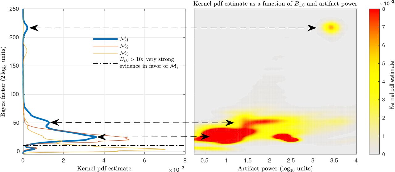
Comparison of generative models with different variants of the artifact dictionary with respect to  . Left: Bayes factor kernel pdf estimate for each artifact model. Right: B1,0 kernel pdf estimate as a function of artifact power.
To that end, we estimated the brain and artifact source time series of all subjects in the testing set under each model. We collected the log evidence afforded by each model in blocks of 40 msec of data and computed Bayes factors with respect to  .
.
The left panel of Fig 3 shows the kernel pdf estimate of each Bayes factor: B1,0, B2,0, B3,0 in blue, orange, and yellow traces respectively. The area above the dotdashed black trace represents the probability space in which modeling artifacts yielded a better generative model for the EEG signal. We computed the probability of having very strong evidence in favor of model  by integrating over Bayes factors higher than 10,
  where fi(Bi,0) denotes a pdf as a function of model
  As shown in Table 1, models
  and
and  yielded the highest probability. Since
  includes
  and
and  henceforth we use the artifact dictionary given by Eq (29).
Artifact model comparison. Probability that there is very strong support in the data in favor of generative model  over
over  , Pi(10 ≤ Bi,0).
To further illustrate the importance of modeling artifact components, the right panel of Fig 3 shows the kernel pdf estimate of B1,0 as a function of the artifact power. The artifact power was calculated as the maximum RMS power over the artifact sources for each 40 msec window. We note that the shape of its pdf depicted on the left panel seems to be determined by the higher performance of the PEB+ algorithm under different clusters of artifactual activity expanding several orders of magnitude.
Fig 4 shows an example of applying PEB+ to an epoch of data of 4 seconds centered around an eye blink event. Panel A shows a 32-channel subset of the raw and reconstructed (cleaned) EEG traces in black and red respectively. In addition to an eye blink, we have a lateral eye movement event around the 1 sec latency. Panel B shows the estimated EOGv and EOGh artifact source activity in blue and orange respectively. We note that these artifact sources are active only at the latencies where the EEG is affected and mostly zero elsewhere. In panel C, the first and last two columns represent the raw and cleaned EEG topographies at the maximum of the lateral eye movement and eye blink events respectively. Panel D shows different views of the estimated cortical source maps underlying the raw topographies in C. The cleaned topographies in C are obtained after the estimated artifact sources are projected out of the data. Panel E shows the log evidence for generative models  and
and  in blue and orange respectively. Note that both traces differ mostly only when artifacts occur and higher log evidence in favor of model
  indicates that source estimation benefits from modeling artifacts.

Example of applying PEB+ to an epoch of EEG with lateral eye movement and eye blink artifacts. A: 32-channel subset of raw and cleaned EEG traces. B: Estimated EOGv and EOGh artifact source activity. C: Columns 1 and 3 and 2 and 4 represent the raw and cleaned EEG topographies at the maximum of the lateral eye movement and eye blink events respectively. D: Different views of the estimated cortical source maps underlying the raw topographies in C. E: Log evidence yielded by PEB+ and PEB algorithms on consecutive 40 msec blocks of data along this epoch.
It is worth noting that, in the last column of panel D, some residual eye blink artifact seems to be mistakenly represented as a small activation in the frontal pole. We point out that, in practice, it may be extremely hard to totally remove artifactual activity because: 1) the use of a lead field matrix derived from a template head model may misfit the anatomy of the subject introducing errors in the L dictionary, 2) errors in the sensor locations can cause the EEG topography to shift with respect to the expected brain and artifact source projections, 3) EMG scalp projections are difficult to characterize due to their variability, as opposed to EOG projections that are more stereotyped, and 4) unmodeled muscle projections, such as those towards the back of the head that were largely ignored in this study. Despite all these issues, Figures 3 and 4 demonstrate that PEB+ can yield reasonably robust source estimates in the presence of artifacts. Furthermore, panel E of Fig 4 suggests that we could use dips in the log evidence to inform subsequent processing stages of artifactual events that were not successfully dealt with.
3.3 Source separation performance
In this section, we investigate the source separation performance of the PEB+ algorithm. To that end, we used the test set to compare PEB+ and Infomax ICA regarding 1) volume conduction unmixing performance and 2) data size requirements for good source separation. We assessed the unmixing performance by calculating the mutual information reduction (MIR) achieved by each algorithm on data blocks of different sizes.
The MIR is an information theoretic metric that measures the total reduction in information shared between the components of two sets of multivariate time series. The mutual information (MI) between two given time series xi,k and xj,k, I(xi, xj), can be defined as the Kullback-Leibler (KL) divergence between their joint and marginal distributions:
 where I(xi, xj) > 0 indicates that processes xi and xj share information while I(xi, xj) = 0 indicates that they are statistically independent such that

We define the MIR of source separation algorithm A with respect to B, as the difference in normalized total pairwise MI (PMI) achieved by each decomposition:
 where
where  and
and  are the set of components yielded by each method and NA and NB are the number of components afforded by each decomposition. We note that to obtain a PMI that is not biased by the number of components, we normalize each summation by the number of unique (i, j) pairs. Here we calculated the MI using the non-parametric kernel pdf estimates of the quantities in Eq (31) for the the multichannel EEG data, the ROI-collapsed sources estimated by PEB+, and the ICs obtained by Infomax.
In Fig 5, the left panel shows a box plot of the MIR of PEB+ and Infomax calculated with respect to the MI of channel data. As indicated by the x-axis, we ran the experiment multiple times varying the data sizes from 0.5 to 500 seconds (∼ 8 minutes). As expected, both algorithms reduce source MI, thereby reversing to some extent the mixing effect of the volume conduction. We see also that, on average, when the MIR is calculated in short blocks of data, PEB+ exhibits higher unmixing performance while Infomax seems to do better on longer blocks. This effect is more clearly represented in the panel on the right, which shows the box plot of the MIR of PEB+ with respect to Infomax. In that panel, distributions with entire positive (orange) or negative (blue) values indicate a significant source c rosstalk reduction performance in favor of the PEB+ or Infomax algorithms respectively. We note that PEB+ better captures transient dynamics for short 0.5-8 sec data blocks.

Source separation performance. Left: Box plot of MIR with respect to channel data computed on blocks of various sizes. Right: Box plot of MIR of PEB+ with respect to Infomax ICA for the same data blocks shown on the left. On each box, the central mark indicates the median, and the bottom and top edges indicate the 25th and 75th percentiles respectively. The whiskers extend to the most extreme data points not considered outliers, and the outliers are plotted individually using the + symbol. On the right, the distributions with entire positive (orange) or negative (blue) values indicate a significant source crosstalk reduction in favor of the PEB+ or Infomax algorithms respectively.
It is worth noting that with PEB+, it is possible to update the unmixing matrix (given by the term  in Eq (10)) on a time-scale of tens of milliseconds because of the regularization induced by the multiple constraints. This allows for adaptation to nonstationary brain and artifact source dynamics. Infomax (and most ICA algorithms) on the other hand, requires larger data blocks to learn a global factorization of mixing matrix and source activations of reasonable quality. Moreover, Fig 5 suggests that the estimation of a global ICA model is suitable for identifying components that remain stationary over the whole experiment, but otherwise, it is suboptimal for capturing transient dynamics.
3.4 Data cleaning performance
In this section, we benchmark the data cleaning performance of the PEB+ algorithm against ASR. The ASR algorithm has gained popularity in recent years for its ability to remove a variety of high amplitude artifacts in an unsupervised manner, thereby enabling automatic artifact rejection for offline as well as realtime EEG-based BCI applications. Since in real data we do not have a ground truth for artifactual activity, we benchmark the methods according to the correlation between raw and cleaned data samples in blocks with negligible or no artifactual activity, where low correlation values indicate needless distortion of the brain activity.
We ran both algorithms for each subject in the test set and collected the following quantities on subsequent blocks of 40 msec: 1) the correlation between raw and cleaned data (computed as the correlation between the correspondent data blocks vectorized across channels and time points) and 2) the maximum RMS artifact power yielded by PEB+ as described in Section 3.2. ASR’s performance depends on multiple parameters, but it has been indicated that the most critical one is the cutoff [Chang et al., 2018]. In the first experiment we used a cutoff equal to 5, which was the default value of EEGLAB’s ASR plugin at the time of this publication.
In Fig 6, the left and right panels show the empirical kernel pdf estimation of the correlation as a function of the artifact’s power for the ASR and PEB+ algorithms respectively. We see that in both methods, the correlation decreases as artifact power increases. This effect is expected and desired because cleaning algorithms are supposed to modify contaminated raw data. Towards low power artifact regions, however, ASR exhibits a significant amount of p robability mass that spreads down to low correlation values while PEB+ seems to have most of its probability mass bounded from below at around 0.8. This result indicates that, at a cutoff of 5, ASR cleaning is overly aggressive to the point of significantly modifying the data in the absence of artifacts. These findings are in agreement to what was recently reported by Chang et al. [2018].

Data cleaning performance. Kernel pdf estimation of the correlation between raw and cleaned data as a function of artifact power. Left: Data cleaned by ASR using cutoff=5 (default). Right: Data cleaned by PEB+. Note that, as expected, in both algorithms the correlation drops as artifacts increase. Towards low amplitude artifacts, however, ASR significantly distorts the data while PEB+ does not.
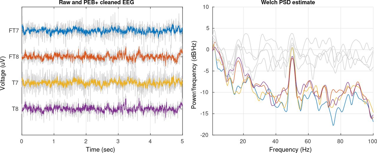
In Section 3.2 we showed that PEB+ can reduce the effects of eye-related artifacts. In Fig 7 we show an example of its performance removing EMG. The data correspond to an excerpt of EEG extracted from a subject selected at random from the test set while he/she was performing the respective cognitive task. In the left panel, the gray and colored traces represent contaminated and cleaned EEG signals respectively. The traces shown correspond to channels located on each side of the cap. Channels in these areas are often contaminated by EMG activity due to their proximity to the temporalis muscle [Fu et al., 2006]. As we can see, the higher amplitude decorrelated EMG activity is largely reduced. In the panel on the right, the gray and colored traces represent the power spectral density estimates of their respective channels on the left. We see that a significant amount of broad band power related to the EMG activity was removed, especially towards frequencies higher than 18 Hz. We note that a strong 50 Hz AC line noise remains in the cleaned data, this is expected because in our approach we do not model this type of artifacts and they can be relatively easily removed using a notch filter.

EMG artifact cleaning. EEG channels contaminated by EMG noise, the gray and colored traces represent raw and cleaned data respectively. Left: Excerpt of EEG signal. Right: Welch power spectral density estimation of the data shown on the left.
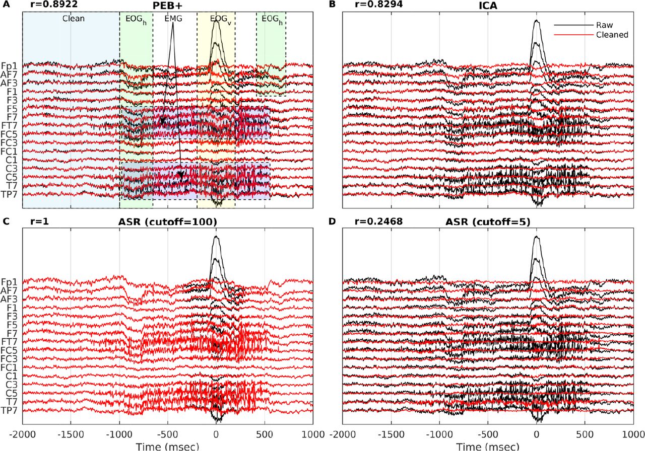
To further illustrate the results of the analysis shown in Fig 6, in Fig 8 we compare the cleaning performance of PEB+ against ASR using two cutoff parameters (5 and 100) and ICA on a typical epoch of EEG containing lateral eye movement, eye blink, and muscle artifacts. As before, the EEG data were extracted from a subject selected at random from the test set. In panel A, the shaded area in blue indicates a segment of clean data, while green, red, and yellow areas indicate segments contaminated by lateral eye movement, muscle, and eye blink artifacts respectively. The correlation achieved by each method (computed by vectorizing all channels and samples in the blue segment) is displayed on the top left corner of each panel. All correlations were significant with p-values lower than 0.005. Panels A, B, C, and D show the raw and cleaned EEG traces produced by PEB+, ICA, ASR (100), and ASR (5) methods respectively. For the ICA approach we cleaned the data by removing the contribution of several stereotypical EOG and EMG components selected manually. PEB+ and ICA displayed similar performance in the sense that lateral eye movement and eye blink artifacts were largely removed, EMG was not totally removed by PEB+, while the clean data segment was minimally distorted, as indicated by correlations with the raw samples of 0.8922 and 0.8294 respectively. We note that the distortion introduced by ICA could be reduced by a more conservative selection of the artifactual ICs to remove. ASR (100) did not distort the clean data segment and removed the higher amplitude eye blink artifact but failed to remove lateral eye movement and muscle artifacts. ASR (5) removed all the artifactual activity, however it also significantly distorted the clean data segment as indicated by a correlation of 0.2468.

Example of the data cleaning performance of PEB+, ICA, and ASR on a noisy epoch. Only 16 channels are shown. A: PEB+. B: ICA. C: ASR with cutoff=100. D: ASR with cutoff=5 (current default value in EEGLAB’s clean_rawdata plugin). In panel A, the segment of data used to compute the correlations between raw and cleaned EEG is indicated with the blue shaded area (−2000 msec to −1000 msec) while the areas shaded in green, yellow and red indicate lateral eye movement, eye blink, and muscle artifacts respectively.
3.5 Heading computation during full-body rotations
We finalize the paper with an application of the PEB+ algorithm to MoBI data. MoBI experiments are notoriously difficult to analyze due to the amount of motion-induced artifacts as well as the presence of transient and stationary brain dynamics of variable duration across trials. Here, we try to replicate the main findings of a study that looked into the dynamics of the retrosplenial cortex (RSC) supporting heading computation during full-body rotations [Gramann et al., 2018].
Heading computation is key for successful spatial orientation of humans and other animals. The registration of ongoing changes in the environment, perceived through an egocentric first-person perspective has to be integrated with allocentric, viewer-independent spatial information to allow complex navigation behaviors. The RSC provides the neural mechanisms to integrate egocentric and allocentric spatial information by providing an allocentric reference direction that contains the subject’s current heading relative to the environment [Byrne et al., 2007]. Single-cell recordings in freely behaving animals have shown that the RSC is also implicated in heading computation [Sharp et al., 2001]. And although there is fMRI evidence that points to the same conclusion in humans that navigate in a virtual environment [Baumann and Mattingley, 2010], verifying this hypothesis in more naturalistic settings has remained elusive.
Recently, Gramann et al. [2018] used EEG synchronized to motion capture recordings combined with virtual reality (VR) to investigate the role of the RSC in heading computation of actively moving humans. Data were recorded from 19 participants using 157 active electrodes sampled at 1000 Hz and band-pass filtered from 0.016 Hz to 500 Hz using a BrainAmp Move System (Brain Products, Gilching, Germany). 129 electrodes were placed equidistant on the scalp and 28 were placed around the neck using a custom neckband. In that study, data from physically rotating participants were contrasted with rotations based on visual flow. In the physical rotation condition, participants wore a Vive HTC head-mounted display (HTC Vive; 2 × 1080 × 1200 resolution, 90 Hz refresh rate, 110° field of view). They were placed in a sparse VR environment devoid of any landmark information facing an orienting beacon at the beginning of each trial. The beacon was then replaced by a sphere that started rotating around them to the left or the right at a fixed distance with two different, randomly selected, velocity profiles on each trial. Participants were instructed to rotate on the spot to follow the sphere and keep it in the center of their visual field. The sphere movement was completed at an eccentricity randomly selected between 30° and 150° relative to the initial heading. When the sphere stopped, they had to rotate back and press a controller button to indicate when they believed to have reached their initial heading orientation. After the button press, the beacon would reappear and participants had to rotate to face the beacon and to start the next trial. In the joystick rotation condition, participants stood in front of a large TV screen (1.5 m viewing distance, HD resolution, 60 Hz refresh rate, 40′′ diagonal size) controlling a gaming joystick to rotate in the same VR environment with an otherwise identical trial structure.
Using an ICA/dipole fitting approach, the data was analyzed with a focus on oscillatory activity of ICs located in or near the RSC. ICs were clustered using repetitive k-means clustering optimized to the RSC as the region of interest. Four subjects without an IC in the RSC were excluded from the analysis (21% of all participants). Subsequently, the wavelet (Morlet) time-frequency decomposition was computed for each IC in the RSC cluster for the rotation periods. The spectral baseline was defined as the 200 msec period before stimulus onset and subtracted from each timefrequency decomposition. To account for different trial durations, single trial time-frequency maps were linearly time-warped with respect to the presentation of the stimulus and rotation onset and offset to create time-warped event-related spectral perturbations (ERSPs). Using this approach, the data from the RSC cluster in the joystick rotation condition replicated previous studies using desktop navigation protocols and comparable data analysis approaches [Gramann et al., 2010, Chiu et al., 2012, Lin et al., 2015, 2018], exhibiting 1) a theta burst between stimulus onset and movement onset and 2) alpha and beta desynchronization during the rotation. The physical rotation, however, had drastically different properties: no clear theta burst was present before movement onset, and only minor desynchronization in higher beta bands, but synchronization in the alpha and low beta bands after movement onset and delta and theta bands during the rotation (see Fig 9 A-B).

Event-related spectral perturbations (ERSPs) in the RSC. Panels A and B are adapted from Gramann et al. [2018]. A: Cluster of IC equivalent current dipoles in or near the RSC. B: ICA derived ERSPs of the joystick and physical rotation conditions and their difference. C: Location of the RSC in the cortical surface of our template. D: PEB+ derived ERSPs of the joystick and physical rotation conditions and their difference. The x-axes at the bottom of panels B and D are annotated with the stimulus onset (Stm), movement onset (Start), percentage of the head rotation cycle, and movement offset (End).
Here, we used the PEB+ algorithm to re-analyze the data. To this end, we further down-sampled the data to 250 Hz, removed the neck channels, applied a 0.5 Hz high-pass forward and backward FIR filter, and subtracted the common average reference. We co-registered each subject-specific 129-channels montage with the head surface of the “Colin27" template, computed each lead field matrix, and linearly warped the A dictionary to the space of the individualized template as explained in Section 3.1.4. Then we ran the PEB+ algorithm for each condition and computed the ERSPs of the centroid source activity (see Eq (15)) within the RSC. The computation of ERSPs was identical to the previous one, only the IC activity of the RSC cluster was replaced by PEB+ RSC source activity of all subjects.
Fig 9 C-D shows the PEB+ group ERSP for the joystick and physical rotation conditions as well as their difference. The top panel shows in red the location of the RSC in our template brain. Despite the differences between the two methodologies, our results largely replicate those in [Gramann et al., 2018] displayed in panels A-B. A few differences between the two results are worth mentioning though. We point out that the differences in ERSP scales exhibited in panels B and D may be explained by different scales of the sources obtained by ICA and PEB+. Also, we note that the low-frequency power increase towards the end of the head rotation cycle in panel D Joystick condition can be explained by artifacts improperly removed near the end of a few trials. It should be emphasized that, unlike the approach used by Gramann et al. [2018], ours has the advantage of using data from all subjects without any cleaning in the time, channel, or trial domains, except for the inherent cleaning capabilities of the PEB+ algorithm. To increase the robustness to residual artifacts, Fig 4 E suggests that a future research direction could explore the use of the log evidence yield by PEB+ to automatically downplay the influence of artifactual trials into post hoc statistical summaries.
Conclusions
In this paper, we have extended the Parametric Empirical Bayes (PEB) framework previously proposed for electrophysiological source imaging [Henson et al., 2011, Wipf and Nagarajan, 2009] in two ways. First, we augmented the standard generative model of the EEG with a dictionary of artifact scalp projections obtained empirically. In our model, we captured EOG, EMG, and single-channel spike artifacts. Second, we used an anatomical atlas to parametrize a source prior that encourages sparsity in the number of active cortical regions, which has the desired property of inducing the segregation of the cortical electrical activity into a few maximally independent components with known anatomical support. We used these elements to develop the PEB+ inversion algorithm. Under the proposed framework, dissimilar problems such as data cleaning, source separation, and imaging can be understood and solved in a principled manner using a single algorithm. Furthermore, we used our framework to point out the connections between distributed source imaging and Independent Component Analysis (ICA), two of the most popular approaches for EEG analysis that are often perceived to be at odds with one another.
We used publicly available data from two independent studies to develop and test the proposed algorithm. In particular, we have shown that PEB+: 1) outperforms classic PEB for source imaging when artifacts are present in the data, while on clean data their performance is comparable, 2) outperforms Infomax ICA for source separation on short blocks of data, thereby showing potential for tracking non-stationary cortical dynamics, and 3) unlike the popular Artifact Subspace Removal algorithm, it can reduce artifacts without significantly distorting epochs of clean data. Furthermore, we were able to replicate the main finding of a study that looked into the dynamics of the retrosplenial cortex (RSC) supporting heading computation during full-body rotations.
The ability to estimate the time series of EEG sources that correspond to known anatomical locations accounting for the influence of artifacts without user intervention, as well as its online adaptation, makes the PEB+ algorithm appealing for established ERP paradigms as well as MoBI. We believe that the proposed algorithm can help to solve basic research questions employing EEG as the functional imaging modality, and at the same time constitute a biologically-grounded signal processing tool that can be useful to translational efforts.
Acknowledgements
This research was supported by NIMH Training Fellowship in Cognitive Neuroscience (AO), UC San Diego Chancellor’s Research Excellence Scholarship (JM, AO), and UC San Diego School of Medicine start-up funds (JM). The PEB+ algorithm is copyrighted for commercial use (UC San Diego Copyright #SD2019810) and free for research and educational purposes.
References


