The covariance perceptron: A new paradigm for classification and processing of time series in recurrent neuronal networks

Abstract

Learning in neuronal networks has developed in many directions, from image recognition and speech processing to data analysis in general. Most theories that rely on gradient descents tune the connection weights to map a set of input signals to a set of activity levels in the output of the network, thereby focusing on the first-order statistics of the network activity. Fluctuations around the desired activity level constitute noise in this view. Here we propose a conceptual change of perspective by employing temporal variability to represent the information to be learned, rather than merely being the noise that corrupts the mean signal. The new paradigm tunes both afferent and recurrent weights in a network to shape the input-output mapping for covariances, the second-order statistics of the fluctuating activity. When including time lags, covariance patterns define a natural metric for time series that capture their propagating nature. Notably, this viewpoint differs from recent studies that focused on noise correlation and (de)coding, because the activity variability here is the basis for stimulus-related information to be learned by neurons. We develop the theory for classification of time series based on their spatio-temporal covariances, which reflect dynamical properties. Closed-form expressions reveal identical pattern capacity in a binary classification task compared to the ordinary perceptron. The information density, however, exceeds the classical counterpart by a factor equal to the number of input neurons. We finally demonstrate the crucial importance of recurrent connectivity for transforming spatio-temporal covariances to spatial covariances.

1 Introduction

A fundamental cognitive task that is commonly performed by humans and animals is the classification of time-dependent signals. For example, in the perception of auditory signals, the listener needs to distinguish the meaning of different sounds: The neuronal system receives a series of pressure values, the stimulus, and needs to assign a category, for example whether the sound indicates the presence of a predator or a prey.

Neuronal information processing systems are set apart from traditional paradigms of information processing by their ability to be trained, rather than being algorithmically programmed. The same architecture, a network composed of neurons connected by synapses, can be adapted to perform different classification tasks. The physical implementation of learning predominantly consists of adapting the connection strengths between neurons —a mechanism termed synaptic plasticity. Learning in artificial neuronal networks is often formulated as a gradient descent for an objective function that measures the mismatch between the desired and the actual outputs. This idea forms the basis of supervised learning [8]. The most prominent examples of such synaptic update rules are the delta rule for the perceptron neuronal network [37, 28, 40] and error back-propagation [38]. These led to modern classification machines, like deep learning and convolutional networks [24, 39]. Their success was only unleashed rather recently by the increased computational power of modern computers and large amounts of available training data, both required for successful training. A key problem to be solved in the improvement of a neuronal information processing is thus to devise new and efficient paradigms for training.

A central feature of the training design is how the physical stimulus is represented in terms of neuronal activity. The traditional view regards the time series of neuronal activity as a succession of snap shots, each of which is possibly corrupted by noise. Thus, the mean activity is regarded as the relevant information of the signal; the variance that measures departures from this mean quantifies the noise. The task of the neuronal network is to robustly classify time-varying input signals despite their variability within each category. This view has led to efficient technical solutions to train neuronal networks by recurrent back-propagation [34] or by back-propagation through time [33].

The representation of information by the mean activity is, however, challenged by two observations in biological neuronal networks. First, neuronal activity in cortex shows a considerable amount of variability even if the very same experimental paradigm is repeated multiple times [2]; neurons also tend to respond more reliably to transients, than to steady states [26]. Previous studies have proposed that this variability may be related to probabilistic representations of the environment in a Bayesian fashion [6, 32]. Second, synaptic plasticity, the biophysical implementation of learning, has been shown to depend upon the temporal activity of the presynaptic and the postsynaptic neurons [27, 7], which can be formalized using the covariance of the neuronal activity [22, 16]. Experimental and theoretical evidence thus points to a relation between the variability of neuronal activity and the representation of the stimulus.

These observations raise several questions: How can a neuronal system perform its function despite this large amount of variability? Moving a step further, can variability even be employed to represent information in its covariance structure, as suggested by covariance-dependent synaptic plasticity and by the preferred response of neurons to transients? If so, how to train networks that employ such representations? Finally, one may wonder if covariance-based learning is superior to technical solutions that employ a mean-based representation, providing a reason why it may be used by neuronal circuits.

We here present a novel paradigm that employs the covariances of fluctuating activity to represent stimulus information. We show how the input-output mapping for covariances can be learned in a recurrent network architecture by efficiently trained the connectivity weights by a gradient-descent learning rule. We find that covariance-based classification is at least as robust as with the mean perceptron. Analyzing the capacity of the network in terms of the maximum number of correctly classifiable stimuli shows that it is en par with the traditional architecture; In terms of memory capacity in bits, however, it largely exceeds the traditional paradigm by a factor m, the number of input neurons. Our work thus provides evidence that covariance-based information processing in a biological context can reach superior performance compared to paradigms that have so far been used in artificial neuronal networks.

The remainder of the article is organized as follows: Section 2 formalizes the main idea of this article, the use of the covariance of stochastic fluctuations to represent information. Section 3 considers a network with feed-forward connectivity that is trained in an online manner, as a time-varying process, to implement a desired mapping from the input covariance to the output covariance. We derive a gradient-descent learning rule that adapts the feed-forward connections and examine the network training in theory, for infinite observation time, as well as for time series of limited duration. Section 4 focuses on the capacity of the covariance perceptron in the case of assigning a binary class label to a bipartite set of noiseless input covariance patterns. This capacity is also compared with the classical perceptron. Section 5 extends the online training of Section 3 to a network with both afferent and recurrent connections. We show how recurrent connections allow us to exploit the temporal structure of input covariances as an additional dimension for stimulus representation that can be mapped to output representations. Importantly, we demonstrate the specific role played by the recurrent network connectivity when the information to learn is in the temporal dimension of covariances, but not in its spatial dimension.

2 Covariance-based representation of information

The present paper considers the problem of information transmission conveyed by a time series in a neuronal network, as illustrated in Fig. 1A. To fix ideas, consider a discrete-time network dynamics as defined by a multivariate autoregressive (MAR) process [25]. The activity of the m inputs is described by a stochastic process in discrete time . The inputs drive the activity of the n output neurons via connections , which form the afferent connectivity. The outputs also depend on their own immediate past activity (i.e. with a unit time shift) through the connections , the recurrent connectivity, as illustrated in Fig. 1A. We define the mean activities where the angular brackets indicate the average over realizations and over a period of duration d.

Figure 1: From mean-based to covariance-based classification of a time series.

A Network with n = 2 output nodes generates a time series (in dark brown on the right) from the noisy time series of m = 10 input nodes (in light brown on the left). The afferent (feed-forward) connections B (green links and green arrow) and, when existing, recurrent connections A (purple dashed links and arrow) determine the input-output mapping. We observe the time series over a window of duration d. B The time series in panel A determines the m-dimensional vector of mean activities, averaged over the observation window d (darker pixels indicate higher values). The classification scheme is implemented by tuning the connectivity weights A and B such that several input patterns of mean activity (m-dimensional vectors on the left-hand side) are mapped to the same output pattern (n-dimensional vector of the right-hand side), thereby representing two categories in red (dotted rectangle, neuron 1 highly active) and blue (neuron 2 highly active). The mapping between input and output (mean) vectors in Eq. (2) corresponds to the classical perceptron. C The covariance perceptron maps the covariance patterns of an input time series (m × m matrices on the left-hand side) to covariance patterns of the output time series (n × n matrices on the right-hand side), see Eq. (3) for their formal definition. Here the two classes are represented by larger variance of either of the two nodes.

A classical assumption is that the information is represented by the mean of each input (see Fig. 1B). By tuning the connection weights, A and B, patterns in the mean input activity can be mapped to desired patterns in the mean activity of the output. The example in Fig. 1B maps a bipartite set of patterns to either of two output patterns, each of which representing one class; the network performs a binary classification of the incoming stimuli. Applying a threshold function to the output yields the classical ‘mean perceptron’ [28].

The present study proposes a different representation of information that employs temporal fluctuations, rather than the mean activity. We thus move from the first-order statistics, the mean, to the second-order statistics, the covariance of the statistical fluctuations of the network activity. The input and output covariances, with being the time lag, are defined as

Here we implictly assume stationarity of the inputs over the window of duration d in Fig. 1A. In this study we consider the case of vanishing mean for covariance-based classification, so the second terms on the right-hand sides disappear in Eq. (3); considerations about a mixed scenario based on both means and covariances will be discussed at the end of the article.

In this setting, the goal of learning is to shape the mapping from the input covariance P to the output covariance Q in the network in Fig. 1A. Building up on the classical ‘mean perceptron’ (Fig. 1B), we use classification as an example to illustrate our theory. The ansatz is that correlated fluctuations across neurons —as defined by covariances in Eq. (3)— convey information that can be used to train the network weights and then classify input time series into categories. Fig. 1C shows the concept of classifying a time series based on patterns in the covariance: The ‘red class’ of input covariance matrices P is mapped by the network to an output, where neuron 1 has larger variance than neuron 2. For the ‘blue class’ of input covariances matrices, the variance of neuron 2 exceeds that of neuron 1.

In particular, we aim to use the ‘covariance perceptron’ to discriminate time series that have a covariance structure that results from the input activity obeying a network dynamics itself. In this case, input and output information are of the same type, which makes the scheme represent and process information in a self-consistent manner. This opens the way to successive stages of information processing as in multilayer perceptrons. This viewpoint on signal variability radically differs from that in Fig. 1B, where the information is conveyed by the mean signal and fluctuations are noise. Conceptually, taking the second statistical order as the basis of information is an intermediate description between the detailed signal waveform and the (oversimple) mean signal. The switch from means to covariances implies that richer representations can be realized with the same number of nodes. We assess in this study how to make use of this enlarged representation space for training and classification.

3 Online learning input-output covariance mappings in feedforward networks

This section presents the concepts underlying the covariance perceptron with afferent connections B only (meaning absent recurrent connectivity A = 0) and compares it with the classical perceptron. The classical perceptron for means, shown in Fig. 1B, corresponds to observing the output mean vector Y for the classification of the input mean vector X in Eq. (2). It relies on the input-output mapping

The derivation of this consistency equation —with A = 0 in Eq. (1)— assumes stationarity for the inputs. Under the same assumption of (second-order) stationarity, the novel proposed scheme relies on the mapping between the input and output covariance matrices, P⁰ and Q⁰ in Eq. (3), namely where T denotes the matrix transpose. Details can be found with the derivation of the consistency equation Eq. (23) in Appendix A, which also assumes stationarity. The common property of Eqs. (4) and (5) is that both mappings are linear in the respective inputs (X and P⁰). However, the second is bilinear in the weight B while the first is simply linear. Note also that this section ignores temporal correlations (i.e. we consider that P¹ = P^−1T = 0); time-lagged covariances, however, do not play any role in Eq. (23) when A = 0.

3.1 Theory for learning of spatial covariance structure by tuning afferent connectivity

To theoretically examine covariance-based learning, we start with the abstraction of the MAR dynamics P⁰ ↦ Q⁰ in Eq. (5). As depicted in Fig. 2A, each training step consists in presenting an input pattern P⁰ to the network and the resulting output pattern Q⁰ is compared to the objective Ǭ⁰ in Fig. 2B. For illustration, we use two categories (red and blue) of 5 input patterns each, as represented in Fig. 2C-D. To properly test the learning procedure, noise is artificially added to the presented covariance pattern; compare the left matrix in Fig. 2A to the top left matrix in Fig. 2C. The purpose is to mimic the variability of covariances estimated from a (simulated) time series of finite duration (see Fig. 1), without taking into account the details of the sampling noise. The update ΔB_ik for each afferent weight B_ik is obtained by minimizing the distance in Eq. (25) between the actual and the desired output covariance where U^ik is a m × m matrix with 0s everywhere except for element (i, k) that is equal to 1; this update rule is obtained from the chain rule in Eq. (26), combining Eqs. (27) and (30) with P^-1 = 0 and A = 0 (see Appendix B). Here η_B denotes the learning rate and the symbol ⊙ indicates the element-wise multiplication of matrices followed by the summation of the resulting elements —or alternatively the scalar product of the vectorized matrices. Note that, although this operation is linear, the update for each matrix entry involves U^ik that selects a single non-zero row for U^ik P⁰ B^T and a single non-zero column for BP⁰U^ikT. Therefore, the whole-matrix expression corresponding to Eq. (6) is different from , as could be naively thought.

Figure 2: Learning variances in a feed-forward network.

A Schematic representation of the input-output mapping for covariances defined by the afferent weight matrix B, linking m = 10 input nodes to n = 2 output nodes. B Objective output covariance matrices Ǭ⁰ for two categories of inputs. C Matrix for the 5 input covariance patterns P⁰ (left column), with their image under the original connectivity (middle column) and the final image after learning (right column). D Same as C for the second category. E Evolution of individual weights of matrix B during ongoing learning. F The top panel displays the evolution of the error between Q⁰ and Ǭ⁰ at each step. The total error taken as the matrix distance E⁰ in Eq. (25) is displayed as a thick black curve, while individual matrix entries are represented by gray traces. In the bottom panel the Pearson correlation coefficient between the vectorized Q⁰ and Ǭ⁰ describes how they are “aligned”, 1 corresponding to a perfect linear match.

Before training, the output covariances are rather homogeneous as in the examples of Fig. 2C-D (initial Q⁰) because the weights are initialized with similar random values. During training, the afferent weights Bik in Fig. 2E become specialized and tend to stabilize at the end of the optimization. Accordingly, Fig. 2F shows the decrease of the error E⁰ between Q⁰ and Ǭ⁰ defined in Eq. (25). After training, the output covariances (final Q⁰ in Fig. 2C-D) follow the desired objective patterns with differentiated variances, as well as small covariances.

As a consequence, the network responds to the red input patterns with higher variance in the first output node, and to the blue inputs with higher variance in the second output (top plot in Fig. 3B). We use the difference between the output variances in order to make a binary classification. The classification accuracy corresponds to the percentage of output variances with the desired ordering. The evolution of the accuracy during the optimization is shown in Fig. 3C. Initially around chance level at 50%, the accuracy increases on average due to the gradual shaping of the output by the gradient descent. The jagged evolution is due to the noise artificially added to the input covariance patterns (see the left matrix in Fig. 2A), but it eventually stabilizes around 90%. The network can also be trained by changing the objective matrices to obtain positive cross-covariances for red inputs, but not for blue inputs (Fig. 3D); in that case variances are identical for the two categories. The output cross-covariances have separated distributions for the two input categories after training (bottom plot in Fig. 3E), yielding the good classification accuracy in Fig. 3F. As a sanity check, the variance does not show a significant difference when training for crosscovariances (top plot in Fig. 3E). Conversely, the output cross-covariances are similar and very low for the variance training (bottom plot in Fig. 3B). These results demonstrate that the afferent connections can be efficiently trained to learn categories based on input (co)variances, just as with input vectors of mean activity in the classical perceptron.

Figure 3: Comparison between learning output patterns for variance and cross-covariance.

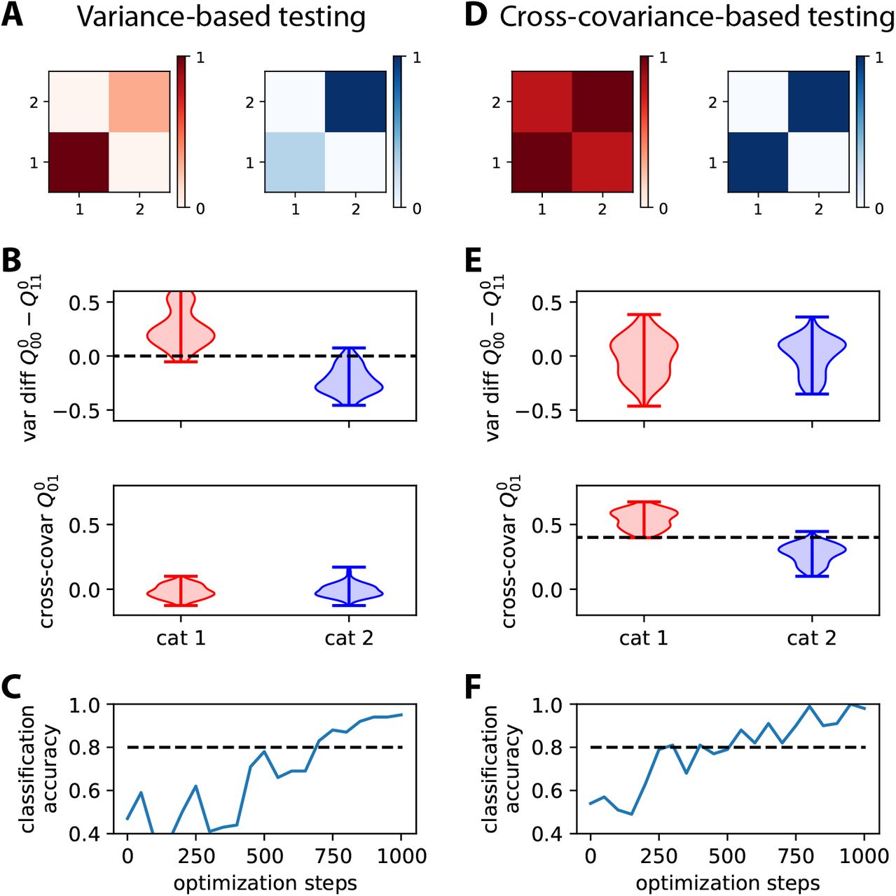
A The top matrices represent the two objective covariance patterns of Fig. 2B, which differ by the variances for the two nodes. B The plots display two measures based on the output covariance: the difference between the variances of the two nodes (top) and the cross-covariance (bottom). Each violin plot shows the distributions for the output covariance in response to 100 noisy versions of the 5 input patterns in the corresponding category. Artificial noise applied to the input covariances (see the main text about Fig. 2 for details) contributes to the spread. The separability between the red and blue distributions of the variances indicates a good classification. The dashed line is the tentative implicit boundary enforced by learning using Eq. (30) with the objective patterns in panel A: Its value is the average of the variance differences over the two categories. C Evolution of the classification accuracy based on the variance difference between the output nodes during the optimization. Here the binary classifier uses the differece in output variances, predicting red if the variance of the output node 1 is larger than 2, and blue otherwise. The accuracy eventually stabilizes above the dashed line that indicates 80% accuracy. D-F Same as panels A-C for two objective covariance patterns that differ by the cross-covariance level, strong for red and zero for blue. The classification in panel F results from the implicit boundary enforced by learning for the cross-covariances (dashed line in panel E), here equal to 0.4 that is the midpoint between the target cross-covariance values (0.8 for read and 0 for blue).

3.2 Online learning for time series observed using a finite time window

Now we turn back to the configuration in Fig. 1C and verify that the learning procedure based on the theoretical consistency equations also works for simulated time series, where the samples of the process itself are presented, rather than their statistics embodied in the matrices P⁰ and Q⁰. We refer to this as online learning, but note that the covariances are estimated from an observation window, as opposed to a continuous estimation of the covariances. As before, the weight update is applied for each presentation of a pattern.

To generate the input time series, we use a superposition of independent Gaussian random variables with unit variance (akin to white noise), which are mixed by a coupling matrix W:

We use 10 patterns P⁰ = WW^T, where W is drawn randomly with f = 10% density of non-zero entries, so the input time series differ by their spatial covariance structure. The network has to classify these patterns based on the variance of the output nodes. The setting is shown in Fig. 4A, where only three input patterns per category are displayed.

Figure 4: Online learning input covariances by tuning afferent connectivity.

A The same network as in Fig. 2A is trained to learn the input spatial covariance structure P⁰ of time series governed by the dynamics in Eq. (7). Only 3 matrices P⁰ = WW^T out of the 5 for each category are displayed. Each entry in each matrix W has a probability f = 10% of being non-zero, so the actual f is heterogeneous across the W. The objective matrices (right) correspond to a specific variance pattern for the output nodes. B Example of simulation of the time series for the inputs (light brown traces) and outputs (dark brown). An observation window (gray area) is used to calculate the covariances from simulated time series. C Sampling error as measured by the matrix distance between the covariance estimated from the time series (see panel B) and the corresponding theoretical value when varying the duration d of the observation window. The error bars indicate the standard error of the mean over 100 repetitions of randomly drawn W and afferent connectivity B. D Evolution of the error for 3 example optimizations with various observation durations d as indicated in the legend. E Classification accuracy at the end of training (cf. Fig. 3C) as a function of d, pooled for 20 network and input configurations. For d ≥ 20, the accuracy is close to 90% on average, mostly above the dashed line indicating 80%. F Similar plot to panel E when varying the input density of W from f = 10 to 20%, with d = 20.

The covariances from the time series are computed using an observation window of duration d, after discarding an initial transient period to remove the influence of initial conditions (corresponding to negative times in Fig. 4B). The window duration d affects the precision of the empirical covariances compared to their theoretical counterpart, as shown in Fig. 4C. This raises the issue of the precision required in practice for effective learning.

As expected, a longer observation duration d helps to stabilize the learning, which can be seen in the evolution of the error in Fig. 4D: the darker curves for d = 20 and 30 have fewer upside jumps than the lighter curve for d = 10. To assess the quality of the training, we repeat the simulations for 20 network and input configurations, then calculate the difference in variance between the two output nodes as in Fig. 3B-C. Training for windows with d ≥ 20 achieve very good classification accuracy in Fig. 4E. This indicates that the covariance estimate can be evaluated with sufficient precision from only a few tens of time points. Moreover, the performance only slightly decreases for denser input patterns (Fig. 4F). Similar results can be obtained while training the cross-covariance instead of the variances.

4 Discrimination capacity for perceptron with afferent connections (offline learning)

The efficiency of the binary classification in Fig. 3 relies on tuning the weights to obtain a linear separation between the input covariance patterns. Now we consider the capacity of the covariance perceptron, namely the number of input patterns that can be discriminated in a binary classification, and compare it with the classical linear perceptron (for mean activity). There are two important differences in the present section compared to Section 3. Here we consider noiseless patterns with offline learning, meaning that the weight optimization is performed using a given number p of patterns (or pattern load) and the classification accuracy is evaluated with the same patterns. In addition, the non-linearity applied to the readout (observed output for classification) is incorporated into the weight optimization. We first present geometric considerations about the input-output mappings for the mean and covariance perceptrons. Then we analytically calculate their capacity using methods from statistical physics and compare the prediction to numerical simulation (similar to Fig. 3).

4.1 Input spaces for mean and covariance patterns

Beside the difference between the input-output mappings in terms of the weights B — bilinear for Eq. (5) versus linear for Eq. (4) — the input space has higher dimensionality for covariances than for means: m(m + 1)/2 for P⁰ including variances compared to m for X. Covariances thus offer a potentially richer environment, but they also involve constraints related to the fact that a covariance matrix is positive semidefinite: for all indices i and j.

To conceptually compare the mean and the covariance perceptron, we consider an example with m = 2 and n = 1, so that the number of free parameters for classification (i.e. the afferent weights) and the dimensionality of the output are the same for both perceptrons. In the mean perceptron linear separability for the vector X is implemented by the threshold on Y₁ = B₁₁X₁ + B₁₂X₂ and corresponds to a line in the plane (X₁, X₂), as represented by the purple line in the left plot of Fig. 5A that separates the red and blue patterns (colored dots). The right plot of Fig. 5A, however, represents a situation where the two categories of patterns cannot be linearly separated. This corresponds to a well-known limitation of the (linear single-layer) perceptron that cannot implement a logical XOR gate [28].

Figure 5: Comparison between input patterns based on mean and covariance.

A Two examples of pattern classification for mean-based decoding. In the left diagram, the two categories can be linearly separated, but not in the right diagram. B The left diagram is the equivalent of the right diagram in panel A for variance-based decoding. The right panel extends the left one by considering the covariance .

The same scheme with variance is represented in the left diagram of Fig. 5B. In this example we have . In the absence of the cross-covariance , the situation is similar to the equation for the mean vector, albeit being in the positive quadrant. This means that the output variance cannot implement a linear separation for the XOR configuration of input variances and , when they are both small or both large for the blue category, one small and the other large for the red category. Now considering , we take, as an example, and equal to 0 or 1 for small or large values, so we obtain for the red patterns and for the blue patterns. Provided the blue values of are smaller than the red values, linear separation is achieved. This leads to the sufficient condition . Provided the weight product B₁₁B₁₂ and have opposite signs and that , a pair of satisfactory weights B₁₁ and B₁₂ can be found. Observing that max(u, 1/u) ≥ 1 for all u > 0, a sufficient condition for separating red and blue patterns is ; the right bound simply comes from Eq. (8).

The increased dimensionality for the inputs related to thus gives an additional “degree of freedom” for the variance-based decoding in this toy example. This is illustrated in the right diagram of Fig. 5B by the purple dashed triangle representing a plane that separates the blue and red dots: The trick is “moving” the upper right blue dot from the original position (light blue with ) in front of the plane to a position behind the plane (dark blue with P^>₁⁰₂ > 0). This toy example suggests that separability for input covariances may have more flexibility than for input means, due to the larger dimensionality.

4.2 Theoretical capacity and information density for decoding based on output cross-covariances

To get a more quantitative handle on the capacity, we now derive a theory that is exact in the limit of large networks m → ∞ and that can be compared to the seminal theory by Gardner [15] on the capacity of the mean perceptron.

So far, the weight optimization and classification have been performed in two subsequent steps, illustrated in Fig. 6A. After training the connectivity to implement a mapping from given input covariance patterns to two objective covariance patterns (left plot), classification is performed by a simple thresholding based on the observed entries of the output matrix (right plot; in practice, it is equivalent to evaluate the difference between the output variances). We now combine these two procedures into one (see the red and blue lines that “push” the dot clouds in Fig. 6B), while focusing on cross-covariances. The reason is simple: Consider a single entry of the readout covariance matrix with 1 ≤ i < j ≤ n. For binary classification, it only matters that the covariance be separable, either above or below a given threshold. For each input pattern indexed by 1 ≤ r ≤ p, we assign a label corresponding to the position of with respect to the threshold, where we define following Eq. (5). We are thus demanding less to the individual matrix entry in Q⁰ than in the previous learning for input-output mapping: It may live on the entire half-axis, instead of being fixed to one particular value. Note that the numbers of −1 and 1 in may not be exactly balanced between the two categories here.

Figure 6: Memory capacity of the covariance perceptron with a single readout (n = 2).

A Schematic representation of B Evolution of the readouts over the optimization that maximizes the soft minimum margin by a gradient descent with η = 4 for m = 50 afferent neurons. Each dot corresponds to one of the p = 20 patterns: red for and blue for . C a D Minimum margin over training; blue: minimum margin given by (9); red: soft minimum margin κ′. D Overlap between the pair of row vectors involved in the calculation of the readout . Symbols from numerical optimization; error bars show standard error from 5 realizations; solid line from theory in the large m-limit, which predicts R₁₂ → 0; see Eq. (C.5). F Total number of classifications relative to the number m of inputs over the effective margin relative to the typical variance of an element of the readout matrix. Symbols from numerical optimization; solid curve from theory in the large m limit given by Eq. (13). Other parameters: m given in legend; f = 0.2; c = 0.5. Numerical results in C and D from maximization of the soft-minimum margin κ′.

Formalizing the classification problem, we fix an element of the readout matrix and draw a random label independently for each input pattern . An important measure for the quality of the classification is the margin defined as

It measures the smallest distance over all from the threshold, here set to 0. It plays an important role for the robustness of the classification [11], as a larger margin tolerates more noise in the input pattern before classification is compromised. The margin of the classification is illustrated in Fig. 6A, where each dot represents one of the p patterns and the color indicates the corresponding category . As mentioned above, we directly train the afferent weights B to maximize κ. This optimization increases the gap and thus the separability between red and blue dots in Fig. 6C. In practice, it is simpler to perform this training for a soft-minimum κ′, which covaries with the true margin κ (9), as shown in Fig. 6D.

The limiting capacity is determined by the pattern load p at which the margin κ vanishes. More generally, we evaluate how many patterns we can discriminate while maintaining a given minimal margin. We consider each input covariance pattern to be of the form with 1_m the diagonal matrix and a random matrix χ^r with vanishing diagonal elements and off-diagonal elements, indexed by (k, l), that are independently and identically distributed as with probability 1 − f and , each with probability f/2, while enforcing symmetry for each χ^r. Here f controls the sparseness (or density) of the cross-covariances. From Eq. (5), the task of the perceptron is to find a suitable afferent weight matrix B that leads to correct classification for all p patterns. This requirement reads, for a given margin κ > 0 and a given entry 1 ≤ i < j ≤ n, as

The random ensemble for the patterns allows us to employ methods from disordered systems [13]. Closely following the computation for the mean perceptron by Gardner [15, 21], the idea is to consider the replication of several covariance perceptrons. The replicas, indexed by α and β, have the same task defined by Eq. (10). The sets of patterns and labels ζ^r are hence the same for all replicas, but each replicon has its own readout matrix B^α. If the task is not too hard, meaning that the pattern load p is small compared to the number of free parameters , there are many solutions to the problem Eq. (10). One thus considers the ensemble of all solutions and computes the typical overlap between the solution B^α and B^β in two different replicas. At a certain load p there should only be a single solution left —the overlap between solutions in different replicas becomes unity. This point defines the limiting capacity .

Technically, the computation proceeds by defining the volume of all solutions for the whole set of cross-covariances as where ∫_S dB integrates over all row vectors that lie on an m-dimensional sphere S —the norm of each row vector of B is set to unity. This constraint leads to a variance of each target neuron which is approximately unity, consistent with the input population. The typical behavior of the system for large m is obtained by first taking the average of over the ensemble of the patterns. It can be computed by the replica trick [13]. The assumption is that the system is self-averaging; for large m the capacity should not depend much on the particular realization of patterns. The leading order behavior for m → ∞ follows as a mean-field approximation in the auxiliary variables , assuming symmetry over replicas and indices. Here measures the overlap between the two row vectors of B^α and B^β involved in the calculation of two replica α and β. The saddle point equations —cf. Eqs. (57) and (58) in Appendix C— admit a vanishing solution for i ≠ j. This result is intuitively clear: The two row vectors must be close to orthogonal, because otherwise the diagonal of the input covariance pattern would cause a non-zero bias of the readout . irrespective of the label ζ^r = ±1. Thus the perceptron would lose flexibility in assigning arbitrary labels to patterns. Fig. 6E indeed shows an overlap close to zero, observed for finite-size networks using numerical optimization.

To take into account the total number of independent binary classification labels relative to the input number m, we define the capacity of the perceptron as where p* is the maximum load when the overlap approaches unity —or equivalently the volume of solutions in Eq. (11) vanishes. Our calculation in Appendix C shows that

At vanishing margin one obtains . For n = 2, a single readout, the capacity is hence identical to the mean perceptron [12]. Moreover, it only depends on the margin through the parameter , which measures the margin κ relative to the standard deviation of the readout. This dependence on κ is identical for the mean perceptron, which was originally analyzed for fc² = 1.

The capacity is shown in Fig. 6F in comparison to the direct numerical optimization of the margin. Comparing the curves for different numbers m of inputs, the deviations between the theoretical prediction and numerical results is explained by finite size corrections —at weak loads, the larger network is closer to the analytical result. However, for the larger network the optimization does not converge at high memory loads, explaining the negative margin; pattern separation is incomplete in this regime.

The replica calculation exposes an intuitive explanation for the equivalence of both perceptrons. For the case n = 2 with two row vectors of B and a single label, the problem becomes isotropic in neuron space after the pattern average —cf. Eq. (46) in Appendix C. As an example, we assume a readout in an arbitrary direction determined by a row vector of B, say . The readout element is given by , which is a simple linear readout of a binary random vector χ_1k —the same as with the mean perceptron.

The memory capacity only grows in proportion to n, again similar to n classical mean perceptrons (i.e. n outputs). Intuitively one could expect it to grow as n(n − 1)/2, the number of classification readouts. It is easy to understand why it is the former: Consider three readout neurons —say i, j, and k— and their corresponding row vectors in B, namely and . The covariance . provides a constraint on . Likewise, the entry provides a second constraint, potentially contradicting with the first. Stated differently, we have n(n − 1)/2 independent constraints, but only mn weights in B. Therefore, there is a tradeoff between more readouts and more constraints for the weights.

Even though the pattern load p at a given margin is identical in the two perceptrons, the covariance perceptron has a higher information density. It is sufficient to compare the cases of a single readout in both cases. The mean perceptron stores the information [21] the number of bits required to express the patterns of m binary variables each. The covariance perceptron, on the other hand, stores bits. Although the calculations in Appendix C ignore the constraint that the covariance matrices must be positive semidefinite, this constraint is ensured when using not too dense and strong entries such that fc ≪ 1, thanks to the unit diagonal. Since only determines the scale on which the margin κ is measured, the optimal capacity can always be achieved if one allows for a sufficiently small margin. In a practical application, where covariances must be estimated from the data, this of course implies a longer observation time d to cope with the estimation error. Under this assumption, the expression for the information density of the covariance perceptron grows ∝ m³, while the former for the mean perceptron only grows with m². If one employs very sparse patterns such that f ∝ m^-1 (an extreme condition), both perceptrons have comparable information content. The dependence on the number of readout neurons n is another linear factor in both cases.

4.3 Comparison of capacity via training accuracy for mean and covariance perceptrons

The analysis in the previous subsection exposed that the capacity of the covariance perceptron is comparable to that of the mean perceptron. To compare and complement the results in Section 3, we use the same optimization as in Figs. 2 and 3, but without additional noise on the presented patterns. We consider mean-based decoding and variance-based decoding for the network N1 with a single output node in Fig. 7A, as well as cross-covariance-based decoding for the network N2 with two output nodes.

Figure 7: Numerical evaluation of capacity using offline learning with non-linearity applied to readout.

A Feedforward networks with afferent connectivity as in Fig. 2A with n = 1 and n = 2 output nodes, referred to as N1 and N2. B Example mean vector X (left) and covariance matrix P⁰ (right) whose density of non-zero elements is exactly f = 20%. Note that the variances are all fixed to 2 while nonzero off-diagonal elements are set to c = 1. C Evolution of the classification accuracy over the noiseless patterns (each color correspond to a number of input patterns to learn). The variability corresponds to the standard error of the mean accuracy over 50 input and network configurations. D Comparison of the classification accuracies as a function of the number of patterns (x-axis). Covariance-based learning is tested in the N2 architecture using the cross-covariance (see panel B), while variance-based learning and mean-based learning are performed with N1. The plotted values are the maximum accuracy for each configuration, whose means are represented in panel C. E Similar plot to panel D for covariance-based learning when varying the sparseness of the input covariance matrices, as indicated by the density f in the legend. The error bars indicate the standard error of the mean accuracy over 50 repetitions. F Similar plot to panel E when varying the number m of inputs in the network (see legend). The number of patterns to learned are given as a fraction of m. The error bars correspond to 20 repetitions.

Here we consider binarized outputs obtained using a threshold function θ, for example for and 0 for for the cross-covariance in the network N2, as in the analytical calculation of the capacity. To incorporate this non-linearity in the gradient descent, we choose objectives and redefine the error E in Eq. (25) in Appendix B as . It follows that becomes a matrix full of zeros when the prediction is correct, whereas erroneous prediction corresponds to ±1 for the output entries that determine the decision, with the sign depending on the category. We consider the same kind of patterns as with the analytical calculation, similar to the right matrix in Fig. 7B where off-diagonal elements are either 0 or c = 1 (we further check that the matrices are non-negative and required to be positive semidefinite). The evolution of the classification accuracy averaged over 50 configurations is displayed in Fig. 7C, where each color corresponds to a given number of input covariance patterns (lower accuracy for more patterns) For each configuration, the maximum accuracy is retained, in line with the offline learning procedure.

The same θ is applied to for variance-based decoding with the network N1. For mean-based decoding, we apply θ to X₁ and use binary input patterns (left vector in Fig. 7B), which corresponds to the classical perceptron. The comparison between the respective accuracies when increasing the total number p of patterns to learn (p/2 in each category) in Fig. 7D shows that the variance perceptron with the N1 network is on par with the mean perceptron. It also shows a clear advantage for the covariance perceptron, which is partly explained by the fact that the N2 network has twice as many afferent weights as the N1 network. The sparseness of the input patterns also affects the capacity that slightly increases for denser covariance matrices in Fig. 7E, as suggested by the theoretical results on information density. Last, Fig. 7F shows that tuning the mapping is robust when increasing the number m of inputs.

5 Online learning of simulated time series with hidden dynamics for both afferent and recurrent connectivities

We now come back to online learning with noisy time series and extend the results of Section 3 to the tuning of both afferent and recurrent connectivities in Eq. (1) with the same application to classification. From the dynamics described in Eq. (1), a natural use for A is the transformation of input spatial covariances (P⁰ ≠ 0 and P¹ = 0) to output spatio-temporal covariances (Q⁰ ≠ 0 and Q¹ ≠ 0), or vice-versa (P⁰ ≠ 0, P¹ ≠ 0, Q⁰ ≠ 0 and Q¹ = 0). The Appendices D.2 and D.3 provide examples for these two cases. As in Fig. 2, we here do not simulate the time series, but instead rely on the consistency equations Eqs. (23) and (24), which are obtained in Appendix A under the assumption of stationary statistics. They demonstrate the ability to tune the recurrent connectivity together with the afferent connectivity, which we further examine now. To do so, we consider simulated time series that differ by their hidden dynamics. By “hidden dynamics” we simply mean that each time series obeys a dynamical equation, which determines its spatio-temporal structure that can be used for classification. Concretely, we use with being independent Gaussian random variables unit variance. This dynamical equation replaces the superposition of Gaussians in Eq. (7) for generating temporally correlated input signals. A class consists of a set of such processes, each with a different choice for the matrix W in Eq. (16), as shown in Fig. 8A. The matrix W itself is not known to the classifier, only the resulting statistics of x that obeys Eq. (16); thus we call this setting “classification of hidden dynamics”. The key here is that P¹ conveys information, but not P⁰. Our theory predicts that recurrent connectivity is necessary to extract the relevant information to separate the input patterns. To our knowledge this is the first study that tunes the recurrent connectivity in a supervised manner to specifically extract temporal information when spatial information is “absent”.

Figure 8: Online learning for input spatio-temporal covariances with both afferent and recurrent connectivities.

A Same network as in Fig. S3A to learn the input spatio-temporal covariance structure, which is determined here by a coupling matrix W between the inputs as in Eq. (16). Here we have 3 input patterns per category. The objective matrices (right) correspond to a specific variance for the output nodes. B The matrices W are constructed such that they all obey the constraint P⁰ = 1_m. C Example of simulation of the time series for the inputs (light brown traces) and outputs (dark brown). An observation window (gray area) is used to calculate the covariances from simulated time series. D Evolution of the error for 3 example optimizations with various observation durations d as indicated in the legend. E Classification accuracy after training similar to Fig. S3D averaged over 20 network and input configurations. For the largest d = 100, the accuracy is above 80% on average (dashed line). The color contrast corresponds to the three values for d as in panel D. F Accuracy similar to E when switching off the learning for the recurrent connectivity A.

Concretely, we here use 6 patterns for W (3 for each category) to generate the input time series that the network has to classify based on the output variances, illustrated in Fig. 8A. Importantly, we choose W = exp(μ1_m + V) with exp being the matrix exponential and V an antisymmetric matrix and μ < 0 for stability. As a result, the zero-lag covariance of the input signals is the same for all patterns of either category, proportional to the identity matrix as illustrated in Fig. 8B. This can be seen using the discrete Lyapunov equation P⁰ = WP⁰W^T + 1_m, which is statisfied because WW^T = exp(2μ1_m + V + V^T) = e^2μ1_m. As mentioned earlier, the time-lagged covariances P¹ = WP⁰ differ across patterns, which is the basis for distinguishing the two categories. The derivation of the consistency equations in Appendix A assumes P² = 0 and is thus an approximation because we have P² = W²P⁰ here. As the input matrix W must have eigenvalues smaller than 1 in modulus to ensure stable dynamics, our approximation corresponds to ||P²|| = ||WP¹|| < ||P¹||.

The output is trained only using Q⁰, meaning that the input spatio-temporal structure is mapped to an output spatial structure. Simplifying Eq. (71) for the current configuration, the weight updates are given by where the derivatives are given by the matrix versions of Eqs. (30) and (32) in Appendix B:

Both formulas have the form of a discrete Lyapunov equation that can be solved at each optimization step to evaluate the weight updates for A and B. The non-linearity due to the recurrent connectivity A thus plays an important role in determining the weight updates. As Eq. (18) involves the approximation of ignoring P², the purpose of the following is to test the robustness of the proposed learning in a practical use.

The covariances from the time series are computed using an observation window of duration d represented in Fig. 8B, in the same manner as before. We use a larger window duration d compared to Fig. 4 because the output covariances are much noisier here due to the approximation mentioned above. The influence of d can also be seen in Fig. 8D, where the evolution of the error for the darkest curves with d ≥ 60 remain lower on average than the lighter curve with d = 20. To assess the quality of the training, we repeat the simulations for 20 network and input configurations, then calculate the difference in variance between the two output nodes for the red and blue input patterns. The accuracy gradually improves from d = 20 to 100 in Fig. 8E. When switching off the learning of A in Fig. 8F, classification stays at chance level. This is expected and confirms our theory, because the learning for B only captures differences in P⁰, which is the same for all patterns here. These results demonstrate the importance of recurrent connections in transforming input spatiotemporal covariances into output spatial covariances.

6 Discussion

This paper presents a new learning theory for the categorization of time series. We derive learning rules to train both afferent and recurrent connections of a linear network model in a supervised manner. The proposed method extracts regularities in the spatio-temporal fluctuations of input time series, as quantified by their covariances. Networks can be trained to map several input time series to a stereotypical output time series that represents the respective class, thus implementing a ‘covariance perceptron’ as shown here for two categories of output covariance patterns.

A main result is that the covariance perceptron can be trained in an online manner to robustly classify time series with various covariance patterns, while observing a few time points only (Fig. 4). Intuitively, this robustness results from the representation of the information by the covariance within a higher-dimensional space compared to the mean, which is employed by classical architectures. The new architecture therefore can make more efficient use of the resources, neurons and synapses, as formally shown by assessing its capacity; the information density is orders of magnitude larger than that of the mean perceptron: It exceeds the mean perceptron by a factor equal to the number of input neurons even though the number of classifiable patterns is theoretically the same as for the classical perceptron (Fig. 6). In simulations akin to offline learning, the resulting accuracy of the covariance perceptron compares favorably with the mean perceptron (Fig. 7). The other main result is the demonstration that the covariance perceptron can classify time series with respect to their hidden dynamics, based on temporal information only (Fig. 8). In other words, the goal here is to distinguish the statistical dependencies in signals that obey different dynamical equations. We stress the importance of the results for online learning: Cross-validation is here performed by taking into account the variability inherent to the time series. This contrasts with the assessment of the capacity that relies on noiseless patterns (Fig. 7).

The conceptual change of perspective compared to previous studies is that variability in the time series is here the basis for the information to be learned, namely the second-order statistics of the co-fluctuating inputs. This view, which is based on dynamical features, thus contrasts with classical and more “static” approaches that consider the variability as noise, potentially compromising the information conveyed in the mean activity of the time series. Importantly, covariance patterns can involve time lags and are a genuine metric for time series, describing the transfer of activity between nodes. This paradigm opens the door to a self-consistent formulation of information processing in recurrent networks: The source of the signal and the classifier both have the same structure of a recurrent network.

6.1 Covariance-based decoding and representations

The mechanism underlying classification is the linear separability of the input covariance patterns performed by a threshold on the output activity, in the same manner as in the classical perceptron for vectors. The perceptron is a central concept for classification based on artificial neuronal networks, from logistic regression [8] to deep learning [24, 39]. The entire output covariance matrix Q⁰ can be used as the target quantity to be trained, cross-covariances as well as variances. In Section 4 the non-linearity on the readout used for classification has been included in the gradient descent. It remains to be explored which types of non-linearities improve the classification performance —as is well known for the perceptron [28]— or lead to interesting input-output covariance mappings. Nonetheless, our results lay the foundation for covariance perceptrons with multiple layers, including linear feedback by recurrent connectivity in each layer. The important feature in its design is the consistency of covariance-based information from inputs to outputs.

Although our study is not the first one to train the recurrent connectivity in a supervised manner, our approach differs from previous extensions of the delta rule [28] or the back-propagation algorithm [38], such as recurrent back-propagation [34] and back-propagation through time [33]. Those algorithms focus on the mean activity (or trajectories over time, based on first-order statistics) and, even though they do take temporal information into account (related to the successive time points in the trajectories), they consider the inputs as statistically independent variables. Moreover, unfolding time corresponds to the adaptation of techniques for feedforward networks to recurrent networks, but it does not take the effect of the recurrent connectivity as in the steady-state dynamics considered here. In the context of unsupervised learning, several rules were proposed to extract information from the spatial correlations of inputs [31] or their temporal variance [4]. Because our training scheme is based on the same input properties, we expect that the strengths exhibited by those learning rules also partly apply to our setting, for example the robustness for the detection of time-warped patterns as studied in [4].

The reduction of dimensionality of covariance patterns —from many input nodes to a few output nodes— implements an “information compression”. For the same number of input-output nodes in the network, the use of covariances instead of means makes a higher-dimensional space accessible to represent input and output, which may help in finding a suitable projection for a classification problem. It is worth noting that applying a classical machine-learning algorithm, like the multinomial linear regressor [8], to the vectorized covariance matrices corresponds to nm(m − 1)/2 weights to tune, to be compared with only nm weights in our study (with m inputs and n outputs). The presented theoretical calculations focus on the capacity of the covariance perceptron for perfect classification (Fig. 6). It uses Gardner’s replica method [15] in the thermodynamic limit, toward infinitely many inputs (m → ∞). We have shown that our paradigm indeed presents an analytically solvable model in this limit and compute the pattern capacity by replica symmetric mean-field theory, analogous to the mean perceptron [15]. It turns out that the pattern capacity (per input and output) is exactly identical to that of the mean perceptron. Its information capacity in bits, however, grows with m³, whereas it only has a dependence as m² for the mean perceptron. The proposed paradigm in large networks therefore reaches an information density that is orders of magnitude higher than that of the mean perceptron.

Both the pattern capacity and information capacity linearly depend on the size of the target population n. The latter result is trivial in the case of the mean perceptron —one simply has n independent perceptrons in that case. However, it is non-trivial in the case of the covariance perceptron, because different entries here share the same rows of the matrix B. These partly confounding constraints reduce the capacity from the naively expected dependence on n(n − 1)/2, the number of independent off-diagonal elements of Q⁰, to n.

Future work should extend the theory of the capacity for noiseless patterns (Fig. 6) to take into account the observation noise, which is inherent to time series, as well as to the here-considered network models. For such noisy patterns, it appears relevant to evaluate the capacity in the “error regime” [9], in which classification is not perfect; our numerical results correspond to this regime (Fig. 7).

6.2 Learning and functional role for recurrent connectivity

Our theory shows that recurrent connections are crucial to transform information contained in time-lagged covariances into covariances without time lag (Fig. 8). Simulations confirm that recurrent connections can indeed be learned successfully to perform robust binary classification in this setting. The corresponding learning equations clearly expose the necessity of training the recurrent connections. For objectives involving both covariance matrices, Ǭ⁰ and Ǭ¹, there must exist an accessible mapping (P⁰, P¹) ↦ (Q⁰, Q¹) determined by A and B. The use for A may also bring an extra flexibility that broadens the domain of solutions or improve the stability of learning, even though this was not clearly observed so far in our simulations.

On a more technical ground, a positive feature of our learning scheme is the surprising stability of the recurrent weights A for ongoing learning (see Appendix D.1). Many previous studies use regularization terms, in biology known as “homeostasis”, to prevent the problematic growth of recurrent weights that often leads to an explosion of the network activity [42, 43]. It remains to be explored in more depth why such regularizations are not needed in the current framework.

The learning equations for A in Appendix B can be seen as an extension of the optimization for recurrent connectivity recently proposed [18] for the multivariate Ornstein-Uhlenbeck (MOU) process, which is the continuous-time version of the MAR studied here. Such learning update rules fall in the group of natural gradient descents [1] as they take into account the non-linearity between the weights and the output covariances. A natural gradient descent was used before to train afferent and recurrent connectivity to decorrelate signals and perform blind-source separation [10]. This suggests as another possible role for A the global organization of output nodes; for example, forming communities of output nodes that are independent of each other (irrespective of the patterns).

6.3 Extensions to continuous time and non-linear dynamics

The MAR network dynamics in discrete time used here leads to a simple description for the propagation of temporally-correlated activity. Extension of the learning equations to continuous time MOU processes requires the derivation of consistency equations for the time-lagged covariances. The inputs to the process, for consistency, themselves need to have the statistics of a MOU process [5]. This is doable, but yields more complicated expressions than for the MAR process.

To take into account several types of non-linearities that arise in recurrently connected networks, one can also envisage the following generalization of the network dynamics

Here the local dynamics is determined by ϕ and interactions are rectified by the function ψ. Such nonlinearities are expected to vastly affect the covariance mapping in general, but special cases, like the rectified linear function, preserve the validity of the derivation for the linear system in Appendix A in a range of parameters. The present formalism may thus be extended beyond the non-linearity applied to the readout (Section 4). Note that for the mean perceptron a non-linearity applied the dynamics is in fact the same as applied to the output; this is, however, not so for the covariance perceptron.

Another point is that non-linearities cause a cross-talk between statistical orders, meaning that the mean of the input may strongly affect output covariances and, conversely, input covariances may affect the mean of the output. This opens the way to mixed decoding paradigms where the relevant information is distributed in both, means and covariances.

6.4 Learning and (de)coding in biological spiking neuronal networks

An interesting application for the present theory is its adaptation to spiking neuronal networks. In fact, the biologically-inspired model of spike-timing-dependent plasticity (STDP) can be expressed in terms of covariances between spike trains [22, 16], which was an inspiration of the present study. STDP-like learning rules were used for object recognition [23] and related to the expectation-maximization algorithm [30]. Although genuine STDP relates to unsupervised learning, extensions were developed to implement supervised learning for spike patterns [20, 35, 19, 14, 41]. A common trait of those approaches is that learning mechanisms are derived for feedforward connectivity only, even though they have been used and tested in recurrently-connected networks. Instead of focusing on the detailed timing in spike trains in output, our supervised approach could be transposed to shape the input-output mapping between spiketime covariances, which are an intermediate description between spike patterns and firing rate. As such, it allows for some flexibility concerning the spike timing (e.g. jittering) and characterization of input-output patterns, as was explored before for STDP [17]. An important property for covariance-based patterns is that they do not require a reference start time, because the coding is embedded in relative time lags. Our theory thus opens a promising perspective to learn temporal structure of spike trains and provides a theoretical ground to genuinely investigate learning in recurrently connected neuronal networks. A key question is whether the covariance estimation in our method can be robustly implemented in an online fashion. Another important question concerns the locality of the learning rule, which requires pairwise information about neuronal activity.

Here we have used arbitrary covariances for the definition of input patterns, but they could be made closer to examples observed in spiking data, as was proposed earlier for probabilistic representation of the environment [6]. It is important noting that the observed activity structure in data (i.e. covariances) can not only be related to neuronal representations, but also to computations that can be learned (here classification). Studies of noise correlation, which is akin to the variability of spike counts (i.e. mean firing activity), showed that variability is not always a hindrance for decoding [3, 29]. Our study instead makes active use of activity variability and is in line with recent results about stimulus-dependent correlations observed in data [36]. It thus moves variability into a central position in the quest to understand biological neuronal information processing.

A Network dynamics describing activity propagation

Here we recapitulate well-known calculations [25] that describe the statistics of the activity in discrete time in a MAR process in Eq. (1), which we recall here:

Our focus are the self-consistency equations when the multivariate outputs are driven by the multivariate inputs , whose activity is characterized by the 0-lag covariances P⁰ and 1-lag covariances P¹ = (P⁻¹)^T, where T denotes the matrix transpose. We assume stationary dynamics (over the observation period) and require that the recurrent connectivity matrix A has eigenvalues in the unit circle (modulus strictly smaller than 1) to ensure stability. To keep the calculations as simple as possible, we make the additional hypothesis that P^±n = 0 for n ≥ 2, meaning that the memory of only concerns one time lag. Therefore, the following calculations are only an approximations of the general case for , which is discussed in the main text about Fig. 8. Note that this approximation is reasonable when the lagged covariances Pⁿ decrease exponentially with the time lag n, as is the case when inputs are a MAR process.

Under those conditions, we define and express these matrices in terms of the inputs as a preliminary step. They obey

Because we assume P^±n = 0 for n ≥ 2, we have the following expressions

Using the expression for R, we see that the general expression for the zero-lagged covariance of depends on both zero-lagged and lagged covariances of :

The usual (or simplest) Lyapunov equation in discrete time corresponds to P¹ =0 and the afferent connectivity matrix B being the identity with n = m independent inputs that are each sent to a single output. Likewise, we obtain the lagged covariance for :

Note that the latter equation is not symmetric because of our assumption of ignoring P_±n = 0 for n ≥ 2.

B Theory for weight updates

We now look into the gradient descent to reduce the error E^τ, defined for τ ∈ {0,1}, between the network covariance Q^τ and the desired covariance , which we take here as the matrix distance:

The following calculations assume the tuning of B or A, or both.

Starting with afferent weights, the derivation of their updates ΔB_ik to reduce the error E^τ at each optimization step is based on the usual chain rule, here adapted to the case of covariances: where η_B is the learning rate for the afferent connectivity and the symbol ⊙ defined in Eq. (6) corresponds to the sum after the element-wise product of the two matrices. Note that we use distinct indices for B and Q^τ. Once again, this expression implies the sum over all indices (i′, j′) of the covariance matrix Q^τ. The first terms can be seen as an n × n matrix with indices (i₁, i₂):

The second terms in Eq. (26) correspond to a tensor with 4 indices, but we now show that it can be obtained from the above consistency equations in a compact manner. Fixing j and k and using Eq. (23), the “derivative” of Q⁰ with respect to B can be expressed as

Note that the first term on the right-hand side of Eq. (23) does not involve B, so it vanishes. Each of the other terms in Eq. (23) involves B twice, so they each give two terms in the above expression —as when deriving a product. The trick lies in seeing that where δ denotes the Kronecker delta. In this way we can rewrite the above expression using the basis n × m matrices U^ik that have 0 everywhere except for element (i, k) that is equal to 1. It follows that the n² tensor element for each (i, k) can be obtained by solving the following equation: which has the form of a discrete Lyapunov equation: with the solution and Σ being the sum of 6 terms involving matrix multiplications. The last step to obtain the desired update for ΔB_ik in Eq. (26) is to multiply the two n × n matrices in Eqs. (30) and (27) element-by-element and sum over all pairs (i₁, i₂) —or alternatively vectorize the two matrices and calculate the scalar product of the two resulting vectors.

Now turning to the case of the recurrent weights, we use the same general procedure as above: We simply substitute each occurrence of A in the consistency equations by a basis matrix, once at a time in the case of matrix products. The “derivation” of Q⁰ in Eq. (23) with respect to A gives where V^ij is the basis n × n matrix with 0 everywhere except for (i, j) that is equal to 1. This has the same form as Eq. (31) and, once the solution for the discrete Lyapunov equation is calculated for each pair (i, j), the same element-wise matrix multiplication can be made with Eq. (27) to obtain the weight update ΔA_ij.

Likewise, we compute from Eq. (24) the following expressions to reduce the error related to Q¹: and

These expressions are also discrete Lyapunov equations and can be solved as explained before.

C Theory for the memory capacity of the covariance perceptron with feedforward connectivity

We consider the mapping P⁰ ↦ Q⁰ in Eq. (5) with P⁰ ∈ ℝ^m×m and y ∈ ℝ^n×n, ignoring the recurrent connectivity in Eq. (20). We want to discriminate p input covariance patterns P⁰, which we denote by with 1 ≤ r ≤ p and assume to be of the form: where 1_m is the m × m identity matrix and each symmetric matri χ^r = χ^T is drawn randomly with

Here we ignore further requirements about being positive semidefinite, which is discussed in the main text. For each input covariance , the corresponding output covariance Q⁰ for the mapping in Eq. (5) is

We want to investigate the maximum number p of patterns that can be discriminated using in a given network defined by the afferent connectivity B. For the readout covariance matrix , we demand the following n(n − 1)/2 constraints for all 1 ≤ i ≤ j ≤ n: with each matrix ζ^r being symmetric as is . The parameter κ plays the role of a classification margin. These conditions require each element of the output covariance matrix to be away from zero by κ, on the side determined by the sign of .

First considering the diagonal elements of , we see that Eq. (38) implies

The distribution of the patterns defined by Eq. (37) implies , so the expected value of output variances implies a normalization for each row vector of B, which we assume to be equal to 1:

This gives another constraint for B, in addition to Eq. (39).

C.1 Gardner’s approach to memory capacity

We now define the volume of solutions B whose p mappings in Eq. (38) satisfy the inequalities and the statistics of the output covariance in Eq. (39):

This equation is the analogue to Gardner’s approach of the perceptron; see [21, Section 10.2, eq. 10.83].

We are interested in the average behavior of in the limit of large m and therefore consider using the replica trick . It leads to the study of the pattern average of the following expression in the limit q → 0:

Therefore, we consider q such systems that have identical realizations of patterns. If there are many solutions to the set of equations, the average overlap between different systems will be small. In case there is only a single solution, the overlap will be unity.

C.2 Pattern average

We then perform the average over the distribution of patterns that obey Eqs. (37) and (39). We rewrite the Heaviside function as such that the pattern average can be described by a cumulant generating function Φ^r of the variable with respect to the statistics of ζ and χ. The constant ι is the imaginary unit. Here we have defined the abbreviations and and used that the p patterns are statistically independent. The function Φ^r can be expanded in cumulants and, in the large-m limit, this expansion can be truncated at the second order in a similar fashion to the mean perceptron [21]. As a result, we obtain with

In the second and third lines we added a single term k = l which is negligible in the large-m limit. We see that the only dependence on the sparseness f and the magnitude c of input covariances is in the form fc² —it does not depend on these two parameters separately. The problem is, moreover, now symmetric in all i < j index pairs. We also observe that the bracket that is multiplied p times does not depend on the pattern index r, so that we only get the bracket to the p-th power.

C.3 Auxiliary field formulation

Starting from Eq. (46), we now define the auxiliary fields as for i < j and α ≠ β. For α = β and i = j we have due to Eq. (41). The field for i ≠ j measures the overlap between input vectors to different units. It contributes to the average value of because the unit diagonal (common to all ) is weighted by . Hence the output will be displaced by irrespective of the realization of for α ≠ β measures the overlap of input vectors in different systems. We denote by the row vectors of matrix B^α defined as to rewrite Eq. (46) as with and . We used that is identical for different patterns , hence we may perform the product over r by taking the p-th power. We express the normalization constraint as

Analogously, we employ this Fourier representation of the Dirac δ to express the constraints defining the auxiliary fields Eq. (48) to obtain with and . In defining we used that the integral factorizes in the index k so that we get m times the same integral for each component .

We are interested in the saddle points of the integrals and search for a replica-symmetric solution. We therefore set for α ≠ β. Then in the limit q → 0 we get which gives rise to the following saddle point equations

The above equations show that we need to find the contribution of and proportional to q as this is the only one surviving in the q → 0 limit.

C.4 Limit q → 0

For replica symmetry, the exponent in simplifies to with and . The replica are coupled by the factor , which renders in an q-dimensional integral. In order to apply the limit q → 0, it is convenient to decouple the replicas by performing the Hubbard-Stratonovich transformation which turns the 2q-dimensional integral into a Gaussian integral over the qth power of a function g_ij(t) that is given by a two-dimensional integral with . The resulting form of allows to take advantage of the q → 0 limit by approximating

C.5 Limiting capacity

We are interested in the limit , which denotes the point where only a single solution is found: the overlap of the readout between replicas is identical to the length of the vector in each individual replicon, so only a single solution is found. So we set and study the limit ϵ_i → 0 for all i ∈ [1, m]. We need to be careful in taking this limit as is singular for ϵ = 0. The saddle-point equations relate derivatives of to tilde-fields, which in turn are defined by . A singularity in at ϵ = 0 therefore implies also a singularity in . These singularities will cancel in the following in the calculation of the capacity.

In the following, we first focus on the fields for i < j: The function lnG_ij depends quadratically on and (see Eq. (49)). By Taylor expansion of Eq. (53) around , one can observe that all odd Taylor coefficients vanish since they are determined by odd moments of a Gaussian integral with zero mean. Therefore, also ln F depends quadratically on and . By rewriting Eq. (58) as and , respectively, and analogously for and , we see that is a solution to the saddle point equations. This solution makes sense as represents a displacement of the Q_ij, therefore a non-vanishing value would hinder the classification. At the point of limiting capacity all replicas find the same solution. Therefore, also the overlap across replica must vanish. Using , an analogous procedure as in Section C.4 can be performed to calculate the term in the q → 0 limit

Then Eq. (57) can be easily solved to obtain

Inserting the solution Eq. (64) into Eq. (58) and using Eq. (62), we get in the limit ϵ_i → 0

For ϵ_k, ϵ_l → 0 the function a_kl(t) goes to negative infinity for and erfc(a_kl(t)) → 2. In this case the nominator in the integrand makes the integral vanish. Therefore, we can restrict the integration range to , where a_kl(t) → ∞ for ϵ → 0, such that we can insert the limit behavior of . Using the limiting capacity follows from

The capacity is identical to the capacity of the mean perceptron. In particular, for κ = 0, we get

D Supplementary results

D.1 Stability of ongoing learning

Fig. S1 illustrates the stability of the learning procedure, both to decrease the error to the best possible minimum and avoid the “explosion” of recurrent weights A, i.e. them diverging to ±∞. Here all 10 input patterns have the same objective matrices, Ǭ⁰ in Fig. S1A-B and a pair Ǭ⁰ and Ǭ¹ in Fig. S1C-D. In both cases, the error firstly decreases then stabilizes, still slowly decreasing. The evolution of the Pearson correlation indicates that the structure of the output(s) remains stable over the optimization, even though the network may not perfectly converge towards the objective(s) in error or Pearson correlation.

The procedure to generate realistic input and objective output patterns in Fig. S1C-D aims to ensure that a solution for A and B exists. Indeed, for usual time series, P⁰ and P¹ are not independent, and the choice of the MAR model for the network dynamics similarly imposes constraints on Ǭ⁰ and Ǭ¹. Nevertheless, we had ~ 15% of the optimizations failing due to an explosion for A. For completely random Ǭ⁰ and Ǭ¹, the conclusion from numerical simulations is that the explosion of A is very likely.

D.2 Shaping output spatio-temporal covariances

As shown in Fig. S2A, we want to tune both B and A to obtain a desired spatio-temporal structure in output. We consider inputs with spatial covariances only (since P¹ = 0) to be mapped to spatio-temporal covariances for . For this purpose, we generalize Eq. (6) to calculate the weight updates for A and B from the errors of both Q⁰ and Q¹:

The matrix “derivatives” are given by Eq. (30), Eq. (33), Eq. (32) and Eq. (34) in Annex A while setting P¹ = P^−1T = 0, which read in matrix form:

Similar to U^ik, the n × m matrix V^ij has 0 everywhere except for element (i, j). The key to evaluate the weight update for A is seeing that the third and fourth lines correspond to the discrete Lyapunov equation that can be solved at each optimization step. As before, we randomly draw 10 input patterns to be classified into 2 categories of 5 each, whose objective matrices Q⁰ and Q¹ are represented in Fig. S2B. A positive outcome is that the weight updates lead to rather stable learning dynamics, even for the recurrent connectivity in Fig. S2C. The stability of ongoing learning while leaving classification aside is examined in Annex D.1, see Fig. S1. Meanwhile, the errors for both Q⁰ and Q¹ decrease and eventually stabilize close to zero in Fig. S2E.

Figure S1: Stability of ongoing learning.

A Evolution of the error for 20 optimizations of networks with m =10 inputs to the n = 3 outputs. Here the objective output covariance matrix Ǭ⁰ is random, as are the 10 random input patterns P⁰ and P¹, but no tuning for Q¹ is performed. The plot is similar to Fig. 2F with the error (matrix distance) and the Pearson correlation between Q⁰ and Ǭ⁰ over all 20 optimizations: The black trace corresponds to the mean over the 20 optimizations and the gray area to the standard deviation. B Example evolution of the afferent and recurrent weights (green and purple traces, respectively) for an optimization. C-D Same as panels A-B for 20 optimizations of the same type of networks with more “realistic” objective pairs Ǭ⁰ and Ǭ¹, as well as P⁰ and P¹ input patterns. Both pairs are generated by a MAR, Eq. (16), which yields the consistency equations P¹ = WP⁰ and P⁰ − WP⁰W^T = 1 for a given W. The plotted values correspond to the mean of the two errors or Pearson correlations for Q⁰ and Q¹.

Figure S2: Shaping output spatio-temporal covariances with both afferent and recurrent connectivities.

A Network architecture with m = 10 input nodes and n = 3 output nodes, the latter being connected together by the recurrent weights A (purple arrow). B Objective covariance matrices for two categories (red and blue). C Evolution of the afferent and recurrent weights (green and purple traces, respectively). D Two examples after training of output patterns Q⁰ and Q¹ in response to two input patterns P⁰, among the 5 in each category. E Evolution of the error for the two output covariance matrices. F After training, the covariances in Q⁰ allow for the discrimination between the two categories, while the structure of Q¹ is similar for the two categories. The plot is similar to Fig. 3. The black surrogate corresponds to forcing A = 0 with the trained B and presenting the blue inputs, demonstrating that the trained A is important in shaping the output structure.

After training, the network maps the input patterns P⁰ in the desired manner for Q⁰ and Q¹, see the two examples in Fig. S2D and the robustness test in Fig. S2F —in a similar manner to Fig. 3. The surrogates (black distribution in Fig. S2F) correspond to setting A = 0 with the trained B, which strongly affects the output covariance (here for blue input patterns). This illustrates the importance of tuning the recurrent connectivity in shaping Q¹, as well as with the discrimination capability for Q⁰.

D.3 Learning input spatio-temporal covariances

Now we consider the “converse” configuration of Fig. S2A where each input pattern is formed by a pair of non-zero P⁰ and P¹, see Fig. S3A. The output is trained only using Q⁰, meaning that the input spatio-temporal structure is mapped to an output spatial structure. This time simplifying Eq. (71), the weight updates are given by Eq. (18), which corresponds to discrete Lyapunov equations that can be solved at each optimization step to evaluate the weight update for A and B.

We first examine the specialization in terms of covariances in Q⁰ as defined by the objectives in Fig. S3C. Here we take input patterns P⁰ that are all identical (left matrices in Fig. S3B) such that the weight specialization must be based on the discrepancies between P¹ across inputs, even though this configuration may not be realistic for simulated time series. The desired outcome after training is obtained as illustrated in Fig. S3C. The surrogates (in black) indicate the importance of the trained recurrent connectivity A, although it appears less strong here than in Fig. S2F. Despite incidental troughs, the classification accuracy increases and eventually stabilizes around 90%. Second, Fig. S3D uses the same procedure for specializing the variances in Q⁰ and shows similar conclusions. Together, these results demonstrate a useful flexibility in tuning the input-output covariance mapping using the MAR network.

Figure S3: Learning input spatio-temporal covariances with both afferent and recurrent connectivities.

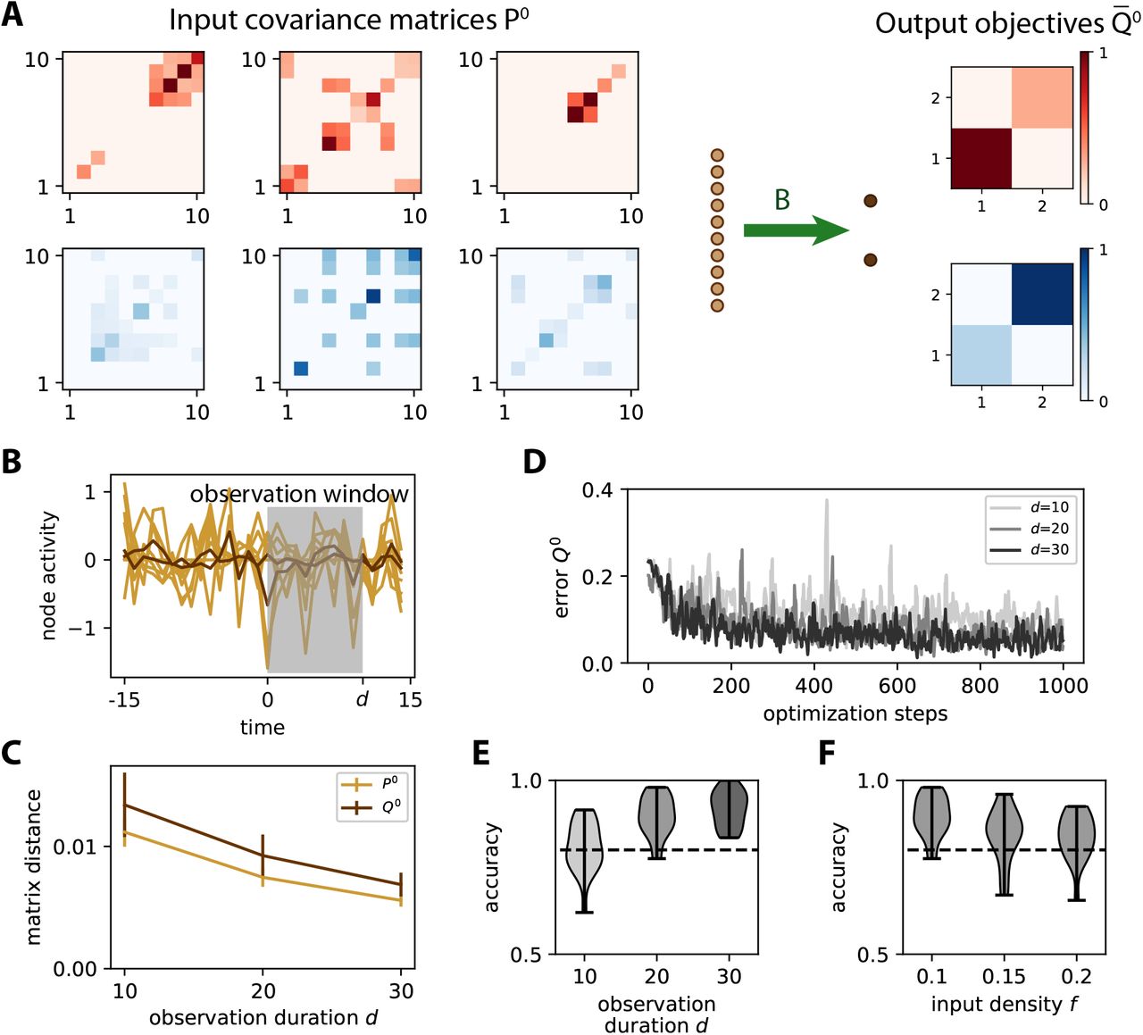
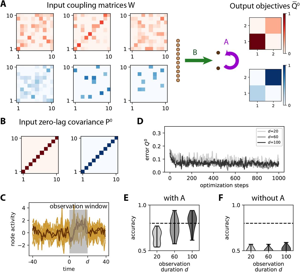
A Similar network to Fig. S2A with m =10 input nodes and n = 2 output nodes. B Two examples of input patterns corresponding to a pair P⁰ and P¹, among the 5 in each category. The P⁰ matrices are identical for all patterns. C Classification based on specializing covariances for the two categories: absent for red and positive for blue (top matrices, same as Fig. 3D). The middle plot is similar to Fig. 3, where the separability of the red and blue distributions indicates the performance of the classification. The comparison between the black and blue distribution shows the importance of the recurrent connectivity A, which is forced to 0 for the surrogates. The bottom plot indicates the evolution of the classification accuracy during the optimization. The binary classification uses the same boundary as in Fig. 3E. D Same as panel C for specializing the variances of the output nodes, with the same objective matrices and classification procedure as in Fig. 3A-B.

7 Acknowledgements

MG acknowledges funding from the Marie Sklodowska-Curie Action (GrantH2020-MSCA-656547) of the European Commission. MG was also supported by the European Unions Horizon 2020 research and innovation programme under Grant Agreement No. 785907 (HBP615SGA2).

This work was partially supported by Helmholtz young investigator’s group VH-NG-1028, the European Union’s Horizon 2020 research and innovation programme under grant agreement No. 720270 (Human Brain Project SGA2), the Exploratory Research Space (ERS) seed fund neuroIC002 (part of the DFG excellence initiative) of the RWTH university and the JARA Center for Doctoral studies within the graduate School for Simulation and Data Science (SSD).

Footnotes

• new result on recurrent connections corrections of typos