

Abstract
The population of the United States is shaped by centuries of migration, isolation, growth, and admixture between populations of global origins. Here, we assemble a comprehensive view of recent population history by studying the ancestry and population structure of over 32,000 individuals in the US using genetic, ancestral birth origin, and geographic data. We identify migration routes and barriers that reflect historical demographic events. We also uncover the spatial patterns of relatedness in subpopulations through the combination of haplotype clustering, ancestral birth origin analysis, and local ancestry inference. These patterns include substantial structure and heterogeneity in Hispanics/Latinos, isolation-by-distance in African Americans, elevated levels of relatedness and homozygosity in Asian immigrants, and fine-scale structure in European descents. Furthermore, quantification of familial birthplaces recapitulates historical immigration waves at high resolution. Taken together, our results provide detailed insights into the genetic structure and demographic history of the diverse US population.
Significance Statement The population of the United States has globally diverse ancestors and a complex history. Despite previous studies of genetic diversity in the US, population history for many groups still remains ambiguous. Here, we study the DNA of over 32,000 US individuals who participated in the National Geographic Genographic Project. By combining analyses of migration, haplotype sharing, and ancestral birthplaces, we reconstruct demographic histories at fine-scale resolution. Among European Americans, Hispanics/Latinos, and African Americans, we disentangle patterns of immigration, within-country migration, and admixture. We also characterize the typically overlooked population history of Asian Americans. Overall, this study sheds light on the complex population histories detailed in the DNA of people living in the US.
Introduction
The United States population is a diverse collection of global ancestries shaped by migration from distant continents and admixture of migrants and Native Americans. Throughout the past few centuries, continuous migration and gene flow have played major roles in shaping the diversity of the US. Mixing between groups that have historically been genetically and spatially distinct have resulted in individuals with complex ancestries while within-country migration have led to genetic differentiation.1–7
Previous genetics studies of the US population have sought to disentangle the relationship between the genetic ancestry and population history of African Americans, European Americans, and Hispanics/Latinos. In African Americans, proportions of African, European, and Native American ancestry vary across the country and reflect migration routes, slavery, and patterns of segregation between states.2,3,8 European American ancestry is characterized by both mixing between different European populations as well as admixture with non-European population.6,9,10 Isolation and expansions in certain European population have also resulted in founder effects.11–13 The mixing of European settlers with Native Americans have contributed to large variations in the admixture proportions of different Hispanic/Latino populations.1,4,5 Among Hispanics/Latinos, Mexicans and Central Americans carry more Native American ancestry; Puerto Ricans and Dominicans have higher African ancestry; and Cubans have strong European ancestry.1,4 Although much effort has been made to understand the genetic diversity in the US, fine-scale patterns of demography, migration, isolation, and founder effects are still being uncovered with the growing scale of genetic data, particularly for Latin American and African descendants with complex admixture history.14,15 At the same time, there has been little research on the population structure of individuals with East Asian, South Asian, and Middle Eastern ancestry in the US.
In addition to being of anthropological interest, understanding fine-scale human history and its role in shaping genetic variation is also important for interpreting the genetic basis of biomedical traits. Currently, these roles are best understood in European populations due to Eurocentric biases in studies.16,17 Consequently, translational interpretability gaps are evident in non-European populations: more variants of unknown significance are identified via genetic testing;18 polygenic risk scores for complex disease risks are much less accurate;17,19 and false positive genetic misdiagnoses are more common.20 Thus, studies of diverse, heterogeneous populations offer substantial value to both our understanding of population history and biomedical outcomes.21
In this study, we comprehensively explore the population structure and migration history of over 32,000 genotyped individuals in the US who partook in the second phase of the National Geographic Genographic Project. The Genographic Project began in 2005 as a not-for-profit public participation research initiative to study human migration history, originally using Y chromosome and mitochondrial markers.22 More recently, it expanded to include autosomal variants.23 Here, we identify patterns of genetic ancestry and haplotype sharing among the project participants. We combine these patterns with ancestral birth origin records and geographic information to uncover recent demographic and migration trends. Taken together, we provide insights into the ancestral origins and complex population histories in the US.
Results
Genetic ancestry and diversity across the United States
To assess proportions and diversity of continental ancestries among individuals in the Genographic Project, we merged genotype data with the 1000 Genomes Project data (Auton et al, 2015) as reference populations, and performed PCA and ADMIXTURE (at K = 2 through K = 9) on the Genographic individuals.24,25 Since self-reported ethnicity does not necessarily reflect genetic ancestry, we sought to objectively assign continental-level ancestry to Genographic individuals. We first trained a Random Forest classification algorithm on the first 10 principal components (PCs) of the 1000 Genome Project individuals using super population classifications (EUR = European, AMR = Admixed American, AFR = African, EAS = East Asian, SAS = South Asian) as ancestry labels (Figure 1A-B; Figure S1). We then used this trained model to assigned continent-level ancestry to each individual in the Genographic cohort at 90% confidence (Table S1; Methods and Materials).
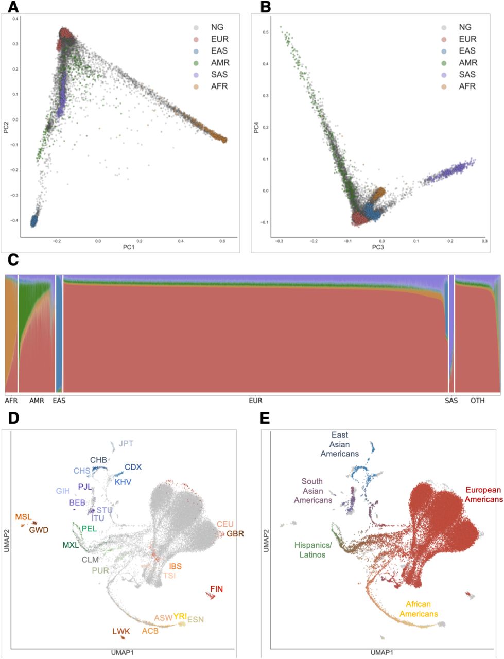
(A) Principal Components Analysis (PCA) of individuals in the United States and in the 1000 Genome Project. Each individual is represented by a single dot. Individuals in this study are colored in grey while 1000 Genome Population individuals are colored by super population (EUR = European, AFR = African, AMR = Admixed American, EAS = East Asian, SAS = South Asian). Principal components (PC) 1 and PC2 are shown.
(B) Similar to (A), with PC3 and PC4 shown.
(C) ADMIXTURE analysis at K=5 of individuals in this study. Each individual was assigned a continent-level ancestry label using a Random Forest model trained on the super population labels and the first 10 PCs of the 1000 Genome Project dataset. OTH = individuals who did not meet the 90% confidence threshold for classification.
(D) UMAP projection of the first 20 PCs. Each dot represents one individual. In (D), individuals in the 1000 Genomes Project are colored by population, while Genographic Project individuals from this study are in grey. In (E), 1000 Genome Project individuals are colored in grey while Genographic Project individuals are colored based on their admixture proportions from ADMIXTURE. The color for each dot was calculated as a linear combination of each individual’s admixture proportion and the RGB values for the colors assigned to each continental ancestry (EUR = red, AFR = yellow, NAT or Native American = green, EAS = blue, SAS = purple). Distances in UMAP do not directly correspond to genetic distance. See Materials and Methods for specific population labels.
Regional differences in genetic ancestry proportions correspond to historical demographic trends. We evaluated the admixture proportions of classified individuals across the four designated US Census regions: South, Northeast, Midwest, and West (Figure 1C; Figure S2). Individuals of European descent make up the majority (78.5%) of the Genographic cohort and are the most prevalent in the Midwest (82.8% of individuals in the Midwest; P<0.01, Fisher’s exact test; Table S1). Individuals classified as having African ancestry are most common in the South (3.2%), followed by the Northeast (3.0%). individuals of Native American ancestry are most prominent in the West and South (9.7% and 7.8% of total individuals in the West and South, respectively; P<0.05, Fisher’s exact test). East Asians mostly reside in the West (2.1%), while South Asians are most abundant in the Northeast (1.0%). A total of 3,028 individuals (9.3% of total) did not meet the classification threshold, although many have ancestry patterns similar to other European individuals (Figure 1C; Table S1). The inability to classify these individuals may be due to the complex and variable admixture profiles of certain populations such as Hispanics/Latinos.
To uncover population substructure, we performed dimensionality reduction with Uniform Manifold Approximation and Projection (UMAP) on the first 20 PCs of a combined Genographic and 1000 Genomes Project dataset.26,27 By leveraging multiple PCs at once, UMAP can disentangle subcontinental structure (Figure 1D-E; Figure S3-S4). Similar to previous analysis,27 populations in the 1000 Genomes Project form distinct clusters corresponding to ancestry and geography. The Genographic individuals project into several clusters, overlapping with the 1000 Genomes Project clusters (Figure 1D-E). Consistent with the PCA and ADMIXTURE analysis, the largest clusters correspond to European ancestry and cluster closely with the 1000 Genomes CEU and GBR populations (CEU=Utah Residents with Northern and Western European Ancestry, GBR=British in England and Scotland).
While UMAP is a visualization tool with no direct interpretation on genetic distance, the continuum of points connecting UMAP clusters reflects the varying degrees of estimated admixture between different continental ancestries. In particular, the complex population structure of Hispanics/Latinos is shown by the points spanning between the clusters of European, Native American, and African ancestry. Coloring of these points based on ancestry proportions affirms the relationship between the degree of admixture and their relative position between reference clusters. Interestingly, African American individuals from both datasets form a single continuum from the European cluster to the Yoruba (YRI) and Esan (ESN) populations of Nigeria in the 1000 Genomes Project, indicative of the West African origins of most African Americans. This observation is consistent with and further expands the previous finding that the African tracts in the admixed 1000 Genomes populations of ACB and ASW were previously found to be similar to the Nigerian YRI and ESN populations.2,19
Population differentiation and migration rate inference across the United States
To better understand the relationship between genetics and geography, we investigated migration rates for genetically inferred Europeans, African Americans, and Hispanic/Latinos across the United States. We excluded East Asians and South Asians due to small sample size and limited our analysis to the contiguous 48 states. We inferred effective migration rates with the estimating effective migration surfaces (EEMS) method,28 which statistically characterizes genetic differentiation via resistance distance across non-homogenous landscapes. By overlaying a dense regular grid of demes and measuring genetic dissimilarities between neighboring demes, EEMS quantifies and visualizes areas with high relative rates of effective migration (colored in blue) and areas with low relative rates of effective migration (also called migration barriers and colored in dark orange).
The inferred migration rates for African Americans reveal genetic signatures of historical demographic events (Figure 2A; Figure S5). Along the Atlantic coast from the Florida Panhandle to southern Maine, we find high effective migration rates, indicating the constant migration and similar effective population sizes of African Americans in these states. However, we also observe a strong north-south barrier to migration starting along the Appalachian Mountain Range, continuing north up the Mississippi River, and extending west across the rest of the country. This migration barrier, along with the migration barrier spanning Texas and New Mexico, reveals a pattern of isolation-by-distance that is consistent with the Great Migration from from the 1910s to the 1960s in which an estimated 6 million African Americans migrated out of the South to cities across the Northeast, Midwest and West.8,29

(A) - (C) Migration rates inferred with EEMS for African Americans (A), Hispanics/Latinos (B), and Europeans (C). Colors and values correspond to inferred rates, m, relative to the overall migration rate across the country. Shades of blue indicate logarithmically higher migration (i.e. log(m) = 1 represents effective migration that is ten-fold faster than the average) while shades of orange indicate migration barriers.
A highly complex pattern of migration exists amongst Hispanics/Latinos with varying migration rates across the country, capturing regional patterns of genetic similarity. Hispanics/Latinos in the southwestern states including two regions bordering Mexico—one in California and another extending from New Mexico to Texas—exhibit high effective migration rates and are separated by a migration barrier in Arizona (Figure 2B; Figure S5). These two distinct regions likely reflect known differences in northward migration from east versus west Mexico.9,30 Along the Atlantic coast from Florida to New York, effective migration has also been fluid. However, barriers to migration are observed west of the Atlantic coast to the Mississippi River, likely resulting from varying admixture proportions.
The pattern of migration for Europeans captures subcontinental structure. Elevated migration rates are observed across most of the country, except for many states in the Midwest and along the Atlantic coast. We find low effective migration rates surrounding Minnesota and North Dakota, potentially due to the genetic dissimilarity of Finnish and Scandinavian ancestry abundant in the region (Figure 2C; Figure S5).9 We also find reduced migration rates across Ohio, West Virginia, and Virginia, suggesting the existence of genetic differentiation along the Appalachian Mountains. Many of the major cities, such as Chicago, Philadelphia, and Miami, are also barriers to migration, perhaps due to higher admixture proportions within cities. The migration barrier encompassing metropolitan New York City may be explained in part by the presence of divergent European populations, such as Ashkenazi Jews (Figure 2C).
Coupling fine-scale haplotype clusters and multigenerational birth records uncovers distinct subcontinental structure
To disentangle more recent and subtle population structure, we performed identity-by-descent (IBD) clustering on the Genographic cohort and annotated clusters using multigenerational self-reported birth origin data. We first built an IBD network from pairwise IBD sharing among 31,783 unrelated individuals. In this network, vertices represent individuals and edges represent the cumulative IBD (in centimorgans, cM) between pairs of individuals. We employed the Louvain method, a greedy heuristic algorithm, to recursively partition vertices in the graph into clusters that maximize modularity at each level of hierarchy.9,31 The clusters of individuals resulting from each iteration can be interpreted as having greater amounts of cumulative IBD shared between individuals within the cluster than with individuals outside of the cluster. At the first level of hierarchy, the full IBD network separated into three clusters: non-European ancestry, Southern Europeans and Ashkenazi Jews, and the rest of the Europeans. Further partitioning, up to four levels of hierarchy, produced clusters with more subcontinental structure. 98% of the 3,028 individuals that were not classified by our Random Forest model were assigned to a haplotype cluster, affirming the power of haplotype clustering for detecting fine-scale structure. No single cluster was overrepresented by unclassified individuals, as unclassified individuals comprised of 8-11% of each cluster.
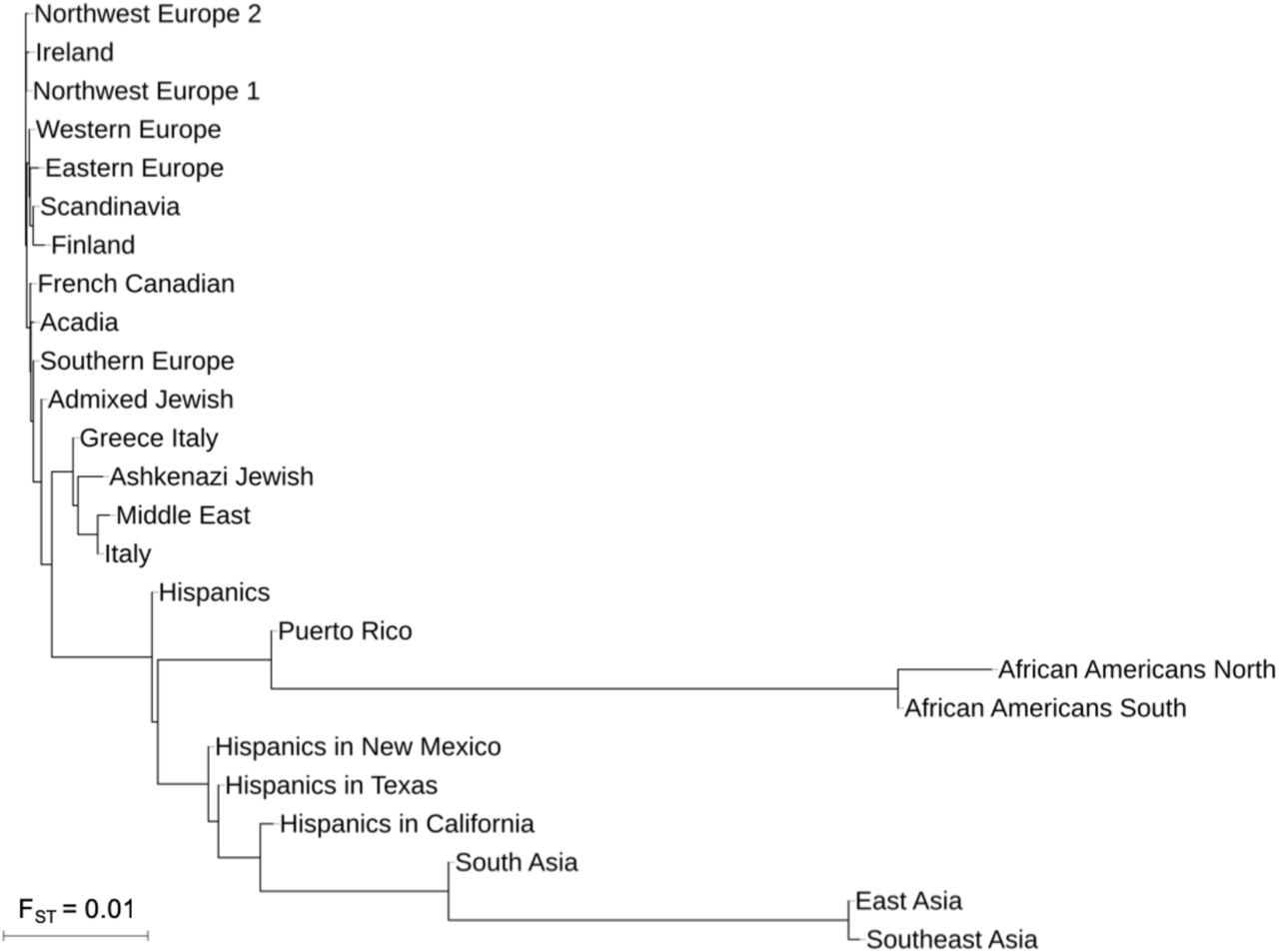
To aid in the interpretation of the clusters, we merged clusters with low genetic differentiation (FST < 0.0001) at the lowest level of hierarchy, resulting in a final set of 25 clusters (Table 1). We annotated each cluster based on ancestral birth origin and ethnicity data and constructed a neighbor-joining tree based on the FST values (Figure 3). As expected, FST values are smallest between European subpopulations (FST=0.0001-0.003) and greatest between clusters of different continental ancestries (FST=0.002-0.09).
Cumulative runs of homozygosity (cROH) was calculated by summing the regions of continuous homozygous segments. Cumulative IBD was determined by summing IBD segments of ≥ 3 cM and filtering for only pairs ≥ 12cM and ≤ 72 cM. Statistics were determined within haplotype clusters, rather than across the ancestrally heterogeneous and imbalanced full network.

Unrooted phylogenetic tree of haplotype clusters was constructed using the neighbor joining method with FST as genetic distance. Negative branch lengths were converted to zero.
Genetic and geographic diversity is greatest amongst Hispanic/Latino haplotype clusters. We identified a total of five Hispanic-related clusters. The largest of these cluster (n=810) is strongly associated with south Florida (OR = 10.4; p = 2.5e-25; Figure 4, Table S4) but is also found in California, and Texas (OR ≥ 2; p < 0.05). No single ancestral birthplace characterizes this cluster, as the US, Mexico, and Cuba each make up more than 10% of the birth origin labels. Proportions of European ancestry tracts inferred with RFMix32 are higher in this cluster (mean = 72.7%, sd=20.4%) than in the other Hispanic/Latino clusters (mean = 48.0% - 67.4%). Puerto Ricans characterize a substantial proportion of another Hispanic/Latino cluster associated with Florida (OR > 4), as well as New York City (OR > 5). Unlike the other Hispanic clusters, the Puerto Rican cluster shares the same branch on the FST tree as the African American clusters, likely due to high proportions of African ancestry (mean = 11.2%, sd = 9.0%) among Puerto Ricans.

(A) Map of counties in which Hispanic/Latino haplotype clusters are enriched. Each dot corresponds to a county, and the size of the dot signifies the number of samples of the particular cluster in that county. Only the Hispanic/Latino cluster with the highest odds ratio is shown for each county, and only the top ten locations with the highest odds ratios are shown for each cluster. Maps showing the full distribution for each haplotype cluster can be found in the supplement (Figure S6).
(B) Ancestral birth origin proportions of each cluster for individuals with complete pedigree annotations, up to grandparent level. Proportions were calculated from aggregating the birth locations of all grandparents corresponding to members of each haplotype cluster. For each chart, only the top five birth origins are shown as individual slices; the remaining birth origins are aggregated into one slice (lightest color).
(C) Ternary plots of ancestry proportions based on local ancestry inference for each haplotype cluster. Each dot represents one individual.
Three distinct clusters of Hispanics were found in the Southwest (Figure 4): one strongly associated with New Mexico (OR > 4; p < 0.05), another primarily in Texas (OR > 3; p < 0.05), and the third associated with Southern California (OR > 2; p < 0.05). Combined with the EEMS analysis, these clusters confirm our observation of parallel migration routes from east and west Mexico into Southwestern United States. While the genetic differentiation of these three clusters are subtle (FST=0.001-0.003), ancestral birth origin patterns and local ancestry proportions for these clusters reveal meaningful dissimilarities. Whereas the majority of Hispanics in New Mexico report US ancestral birth origins through grandparents, the recent ancestors of Hispanics in Texas are predominantly from Mexico. Nonetheless, these two clusters share similar local ancestry proportions with only slight genetic dissimilarity that result in a moderate decrease in migration rate (from darker blue to light blue in Figure 2B). The reduced migration rate along the Texas-Mexico border may be caused by more recent immigrants. Unlike the Hispanic clusters associated with New Mexico and Texas, the Hispanics in California cluster contain greater proportions of ancestors from Central and South American (e.g., Colombia and El Salvador). Proportions of Native American ancestry is also highest in this cluster (Figure 4). Taken together, these two differences further explain the presence of the migration barrier in Arizona between the Hispanics in the California and the Hispanics in New Mexico.
Historical immigration of Europeans into the US occurred in successive waves, with Northern and Western Europeans making up one wave from the 1840s to 1880s and another wave comprising of Southern and Eastern Europeans occurring from the 1880s to 1910s.33 Consistent with this immigration pattern, haplotype clusters with ancestries from Northwest and Central Europe have higher proportions of US ancestral birth origins than haplotype clusters from Southern and Eastern Europe, suggesting earlier immigration (Figure 5). The two clusters with the highest proportion (>75%) of US ancestral birth origin (“Northwest Europe 1” and “Northwest Europe 2”) have approximately 4.5% of UK ancestral origins. The Central European cluster and the Irish cluster both have approximately 66.1% to 68.5% of US grandparental origins, respectively. In contrast, the US makes up only 62.2% and 34.5% of grandparental birth origin for the clusters of Southern Europeans and Eastern Europeans, respectively.

(A) Geographic distributions of haplotype clusters corresponding to regional European ancestries. Each county containing present-day individuals is represented by a dot. The top 20 locations with the highest odds ratio are shown for each cluster. Maps showing the full distribution for each cluster can be found in the supplement (Figure S6).
(B) Ancestral birth origin proportions for each cluster in (A). Only individuals with complete pedigree annotations, up to grandparent level, are included. For each chart, only the top five birth origins are visualized as individual slices; the remaining birth origins are aggregated into one slice (lightest color).
Unlike the larger European clusters, the smaller European clusters reflect the structure of more recent immigrants and genetically isolated populations. The geographic distribution of these subpopulations are more concentrated, and their ancestral birth origin proportions are overrepresented by specific countries and ethnicities (Figure 6). For example, Finns and Scandinavians are abundant in the Upper Midwest and Washington; French Canadians are found in the Northeast; Acadians are present in the Northeast and Louisiana; and Italians, Greeks, Ashkenazi Jews, and Admixed Jews are mostly located in the metropolitan area of New York City. Of the European clusters, median cumulative IBD sharing and cROH lengths are highest amongst Ashkenazi Jews (31.8cM and 11.3 Mb, respectively; Table 1). The two Jewish-related clusters were identified using self-reported ancestral ethnicity data rather than birth origin data, since Jewish ancestry is not specific to any single location. Jewish ancestry, particularly Ashkenazi Jewish ancestry, was more consistently reported on both sides of the family in the larger Jewish cluster (“Ashkenazi Jewish”), suggesting that individuals are more admixed in the smaller cluster (“Admixed Jewish”).

(A) Present-day location of individuals in clusters of more genetically isolated European populations, similar to Figure 5A. For clarity, the top ten locations with the highest odds ratio are shown for each cluster.
(B) Ancestral birth origin proportions for each cluster in (A). Only individuals with complete pedigree annotations, up to grandparent level, are shown. For each chart, only the top five birth origins are shown as individual slices; the remaining birth origins are aggregated into one slice (lightest color).
We inferred two haplotype clusters of African Americans separated along a north-south cline, recapitulating the EEMS migration barrier inference. One cluster is primarily distributed amongst the northern and western states (“African Americans North”) while the other is distributed amongst the states southeast of the Appalachian Mountains (“African Americans South”) (Figure S7). The proportion of US birth origin is higher in the northern cluster than the southern cluster, further evidence of isolation by distance amongst African Americans in the north.8 These two clusters share similar cROH lengths but differ in admixture proportions and median IBD sharing, pointing to a cluster with consistent African American ancestors and a cluster with more admixed ancestors. Median IBD sharing is higher amongst African Americans in the south (median IBD = 19.6 cM, median cROH = 3.3 Mb) than in the north (median = 15.9 cM, Table 2) while the average proportion of African ancestry is higher in the northern cluster than the southern cluster.
Smaller haplotype clusters in the Genographic cohort reflect more recent immigration of South, Southeast, and East Asian individuals to the US, which grew rapidly in the mid-20th Century after the passage of laws eliminating national origin quotas.34 We identified four clusters with birth origins enriched from Asia (Figure S8). The recency of immigration among these clusters is indicated by the less than 30% of ancestral birth origins coming from the US. Geographically, individuals in these clusters primarily reside in major cities. East Asians predominantly inhabit the metropolitan areas of coastal states in the West and Northeast (OR > 2), while South Asians are strongly associated with the Northeast (OR > 2.5). Southeast Asians (OR > 2.5) are enriched in the west but are also associated with the Carolinas and Ohio. Despite its small size, the cluster of Middle Eastern individuals reflects many of the known demographic patterns of Arab Americans, as individuals in this cluster are primarily of Lebanese origin and are distributed in the Northeast as well as metropolitan Detroit. cROH lengths are particularly long for South Asians (median cROH = 10.3 cM), Southeast Asians (median cROH = 7.8 cM), and Middle Easterners (median cROH = 8.2 cM), potentially reflecting inbreeding patterns found in their ancestral regions.35
Discussion
As the US population is becoming increasingly diverse, genomic studies are simultaneously growing in scale and relevance; to increase scientific and ethical parity, these studies must therefore move beyond the current practice of evaluating genetically homogenous groups in isolation.17 Here, we provide an integrative framework for analyzing population structure in ancestrally heterogeneous individuals. Using data from the National Geographic Genographic Project, we untangled the recent demographic histories of European, African American, Hispanic/Latino, and Asian populations in the US by evaluating their admixture proportions, migration rates, haplotype sharing, and ancestral birth origins.
Our comprehensive approach has allowed us to capture spatial patterns of gene flow within and between subpopulations that are difficult to infer from a single method alone. For example, EEMS is limited in identifying unique subpopulations, while haplotype clustering cannot assign admixed individuals partial membership to multiple clusters. An integrative approach can thus enable greater insights into populations with complex histories, such as recently admixed US Hispanics/Latinos.
Consistent with prior studies,4,10 the recent demographic history of Hispanic/Latino populations is complex. Large variations in admixture proportions within and between subpopulations are reflected by US Census Data and can likely be explained by numerous inferred migration barriers. For example, regional differences in the Southwest are highlighted by an inferred migration barrier in Arizona and distinct haplotype clusters surrounding this region. These differences are likely due to higher proportions of Native American ancestry as well as more Central and South American origins in the California Hispanic cluster compared to other southwestern Hispanic/Latinos. Interestingly, although the New Mexico Hispanic/Latino cluster is distinct from the Texan cluster, high levels of gene flow are inferred from southern New Mexico to central Texas, suggesting that certain individuals in these two clusters are genetically similar and may share an ancestral origin (i.e. Mexico). In contrast, those in northern New Mexico are more genetically differentiated, as indicated by a migration barrier, but share the same cluster; these are likely Nuevomexicanos, descendants of Spanish colonial settlers.
The fine-scale population structure of African Americans also reflects known historical events following the transatlantic slave trade, during which millions of West Africans were forcibly moved to the Americas. Subsequently, the movement of African Americans during the Great Migration has been shown to correlate with current patterns of relatedness across US census regions.8 Our results show barriers to migration and gene flow at fine-scale, particularly along the Appalachian Mountains. A north-south migration barrier is also present west of the Mississippi River, and is further supported by the north-south locations of two African American clusters that emphasize this divide. The southern African American cluster contains more recent ancestors outside the US, particularly of Caribbean origin, than the northern African American cluster. These genetic signatures illustrate the impact of recent migration patterns on modern population structure.
Our ability to identify population structure for certain ancestries is subject to participation among individuals from those groups. In particular, individuals with Asian ancestries account for over 5% of US population, but they are underrepresented in US population genetics studies, hindering the investigation of their ancestry in prior studies.9 Our analyses of East Asian, Southeast Asian, South Asian, and Middle Eastern populations therefore provide initial insights into their genetic structure. The ancestral origins and geographic distributions of these clusters are consistent with US Census reports. Since these populations descend from more recent immigrants, the observed patterns of homozygosity within several of these clusters likely reflect consanguinity patterns in some of their ancestral regions. Specifically, the long cROH in South Asians may reflect endogamy for example related to the caste system in India, while similar patterns among the Middle Eastern and Southeast Asian clusters may be capturing consanguineous marriage practices in those regions.36–38 Given the small size of these clusters, however, further studies with larger data are needed.
Population history in the US is best characterized among the most populous European descent individuals. Genetic diversity tends to be highest in more densely populated regions, likely due to the presence of multiple subpopulations in the same place. Many of the European subpopulations we identified are similar to those previously found—e.g., French Canadians, Acadians, Scandinavians, Jews (Supplementary Discussion).9 The geographic distribution of these subpopulations, particularly those that are more genetically diverged, overlap in the metropolitan areas in the Northeast, Midwest, and California.
The emergence of biobank-scale genomic data is enabling more complete pedigrees,39 greater discoveries of fine-scale population structure, and more precise insights into health-related associations. An estimated 26 million people have taken a direct-to-consumer ancestry test,40 indicating widespread interest in ancestry and heritable factors. As participation in genetic studies increase, especially in the US with the All of Us Research Program, so does the need for inferring increasingly granular demographic history in study cohorts. Understanding such genetic structure is important to account for stratification, prevent the overgeneralization of results, and avoid exacerbating existing biases.16,17 This study demonstrates the potential of coupling genetic data with geographic and birth origin data to reconstruct such demographic histories, particularly in a large and heterogeneous population.
Materials and Methods
Human Subjects
The Genographic Project and Geno 2.0 Project received full approval from the Social and Behavioral Sciences Institutional Review Board (IRB) at the University of Pennsylvania Office of Regulatory Affairs on April 12, 2005. The IRB operates in compliance with applicable laws, regulations, and ethical standards necessary for research involving human participants. All data in this study came from participants that consented to have their results be used in scientific research. All data was deidentified.
In addition to genotype data, participants also provided information on geographic location, ancestral birth origin, and self-declared ethnicity. Geographic location was collected in the form of postal code. We limited our analysis to include only individuals who provided valid geographic location. Both ancestral birth origin data and self-declared ethnicity data were collected up to the grandparents of the participants. Approximately 60% of individuals provided complete pedigrees.
Genotyping and Quality Control
Participants of the Genographic project were sequenced with the GenoChip array,23 a Illumina iSelect HD custom genotyping bead array with approximately 150,000 Ancestry Informative Markers from autosomal DNA, Y chromosome DNA, and mitochondrial DNA.
Raw genotype data was quality controlled (QC) using PLINK v1.90b3.39.41 We filtered for samples with ≤ 0.1 missingness, sites with = 0.0 missingness, and MAF ≥ 0.05. After QC, 32,589 individuals and 108,003 sites remained.
Principal Component Analysis
We performed principal component analysis on the quality-controlled samples using FlashPCA version 2.0.25 We included the genotypes of all 2,504 individuals from the 1000 Genomes Project as reference samples. We first found the subset of SNPs (108,003) that were shared between the Genographic samples and the 1000 Genomes Project samples. We next computed PCs across all 108,003 sites for all 1000 Genome Project individuals. Using the resulting PCs, we then projected the Genographic individuals on the same principal component space.
Continental Ancestry Assignment
We assigned continental ancestry to each individual in the Genographic dataset by leveraging the PCs and known super population assignment (AFR=African, EUR=European, EAS=East Asian, AMR=American, and SAS=South Asian) of each individual in the 1000 Genome Project. We trained a random forest classifier on the first 10 PCs of the 1000 Genome Project samples and assigned ancestry to all of the Genographic samples at 90% probability based on the model. All unassigned ancestries were considered “other” (OTH).
Genetic Ancestry Proportion Estimation
We estimated admixture proportions using ADMIXTURE.24 Similar to the PCA analysis, we included the genotypes of all individuals from the 1000 Genomes Project and used the subset of SNPs shared between the Genographic and 1000 Genomes Project datasets. We ran ADMIXTURE for k=3-10 by first analyzing the 1000 Genomes Project in unsupervised mode to learn allele frequencies and obtain ancestry proportions. Then, we projected the Genographic samples onto the learned allele frequencies of the 1000 Genome Project samples to obtain the learned clusters and ancestry proportions. We chose k = 5 as the most stable and best representation of ancestry.
UMAP
We applied the Uniform Manifold Approximation and Projection (UMAP) method to visualize subcontinental structure.26,27 We first combined the PCs for the Genographic samples and the 1000 Genome Project samples, from the PCA analysis above, into one dataset. We then used the UMAP implementation in Python to dimensionally reduce the first 20 PCs from the joint dataset into a two-dimensional plot. We tested various parameter choices for UMAP and found that the default nearest neighbor value of 15 and the minimum distance values of 0.5 delivered the clearest result.
To help with interpretability, we colored the 1000 Genome Project samples in the UMAP projection based on their country level assignments (Figure 1C left). We also visualized the Genographic samples in the UMAP projection by coloring each sample based on their ancestry proportions from ADMIXTURE (Figure 1C right). Specifically, the color (RGB value) of each sample is a linear combination of the sample’s ancestry proportions and the RGB values of each ancestry’s color (EUR = red, AFR = yellow, NAM = green, EAS = blue, SAS = purple).
Genetic Relatedness
We used KING v2.0 to identify the set of unrelated individuals within the Genographic dataset separated by at least two degrees of relatedness.42 In total, 806 individuals had kinship coefficients greater than 0.0884 and were removed for downstream EEMS analysis and haplotype construction and clustering.
Estimating Effective Migration Surfaces
We estimated migration and diversity relative to geographic distance using the estimating effective migration surfaces (EEMS) method.28 We applied EEMS to Genographic individuals that were classified under African, European, and Native American ancestries. We excluded East Asian and South Asian ancestries due to low sample size and population density. We first computed pairwise genetic dissimilarities for all unrelated individuals with available postal code data in each of the three ancestries using the bed2diffs tool provided with EEMS. We then ran the EEMS algorithm with the runeems_snps tool and set the number of demes to 500. Per the recommendation in the manual, we adjusted the variance for all proposed distributions of diversity, migration, and degree-of-freedom parameters such that all were accepted 10%-40% of the time. We increased the number of Markov chain Monte Carlo (MCMC) iterations until the MCMC converged.
Haplotype Calling and Network Construction
We used IBDSeq version r1206 to generate shared identity-by-descent (IBD) segments from genotype data for all unrelated individuals.43 Unlike other algorithms for IBD detection, IBDseq does not reply on phased genotype data and therefore is less susceptible to switch errors in phasing that can cause erroneous haplotype breaks. We filter individual IBD segments by length, excluding those shorter than 3cM. We also removed IBD segments that overlapped partially or fully with long regions (1 Mb) of the chromosome that exhibited no SNPs across all unrelated individuals in the Genographic dataset. These sites can result in false positives IBD sharing and likely correspond to centromeres and telomeres.
We calculate the cumulative IBD sharing between individuals by summing the length of all shared IBD segments. We limit our analysis to pairs of individuals in which cumulative IBD sharing is ≥12 cM and ≤72 cM, as previously described.9 We then constructed a haplotype network of unrelated individuals by defining each node as an individual and the edge connecting two vertices as the cumulative IBD sharing between two individuals, as a proportion of total possible IBD sharing. For comparison, we also constructed an network without filtering for minimum or maximum IBD sharing.
Detection of IBD Clusters
To identify clusters of related individuals in the haplotype network described above, we used the Louvain Method for community detection implemented in the igraph package for R. Briefly, the Louvain Method is a greedy iterative algorithm that assigns vertices of a graph into clusters to optimize modularity (a measure of the density of edges within a community to edges between communities). The Louvain Method begins by first assigning each node as its own community and then adds node i to a neighbor community j. It then calculate the change in modularity and places i in the community with that maximizes modularity. The algorithm terminates when no vertices can be reassigned.
We partitioned the haplotype network into clusters by recursively applying the Louvain Method within subcommunities. At the highest level, we take the full, unpartitioned haplotype graph and identify a set of subcommunities. We isolate the vertices within each subcommunity, keeping only the edges between those vertices to create separate new networks. We then apply the Louvain Method to the new subgraphs. We repeat this process up to four levels. We combined subcommunities with low genetic divergence based on FST values of < 0.0001 (see Genetic Divergence) and arrive at a total of 25 clusters for the filtered network (≥12 cM and ≤72 cM). For the unfiltered network, we arrived at 32 clusters, 4 of which contained less than 10 individuals and were removed from subsequent analyses.
Annotation of IBD Clusters
We used a combination of ancestral birth origins and self-reported ethnicities to discern demographic characteristics of each cluster. For each cluster, we quantified the proportion of each birth origin (i.e. country of origin) amongst all four grandparents, treating each grandparent’s origin equality. We use these proportions to inform population labels. Clusters in which a single non-US birth origin was in high proportions was labeled with that country. In cases where multiple non-US birth locations exists in approximately equally high proportions, we assigned a label representing the broader region (e.g. Eastern Europeans for Poland, Lithuania, Ukraine, and Slovakia; East Asia for Japan, China). For certain clusters, annotations could not be easily discerned by birth origin data. In these cases, we relied on self-reported ethnicities to label the clusters as these populations were found to be less associated with a non-US country (e.g. Ashkenazi Jews) or the population has resided in the US for generations (African Americans, Acadians).
Annotations for the 25 clusters from the filtered network were found to be more interpretable than annotations for the 28 clusters from the unfiltered networks. Specifically, many of the clusters from the unfiltered networks exhibited similar proportions of ancestral origins or ethnicities and were difficult to differentiate (Table S2 and S3). Certain populations (e.g. Finns, Middle Easterners) found from the filtered network were also not identified from the unfiltered network. We therefore used the 25 clusters from the filtered network in downstream analyses.
Mapping IBD Clusters
We mapped individuals using their present-day geographic location. We aggregated individuals from the same county using the postal code to county FIPS code mapping provided by the US Census, and we identified the longitude and latitude points of each county using the same data from the US Census. We then counted the number of individuals at each coordinate for each ancestry.
To identify locations where a cluster is enriched, we performed a Fisher’s exact test for each location and ancestry to obtain an odds ratio and significance value. For each cluster, we mapped only counties with statistically significant (p<0.05) enrichment and an odds ratio (OR) of greater than 1. The size of the circles is scaled to the number of individuals in each location.
Runs of Homozygosity
We used PLINK v1.90b3.39 to infer runs of homozygosity with a window of 25 SNPs.41 We calculated the cumulative runs of homozygosity (cROH) size by summing the lengths of homozygous segments.
Haplotype Estimation
Genographic genotypes were phased with the Sanger Imputation Service using EAGLE2 and the Haplotype Reference Consortium reference panel.44 No genotype imputation was performed.
Local Ancestry Inference
We inferred local ancestry with RFMix v1.5.4 for Genographic samples in haplotype clusters that were annotated as Hispanics/Latinos and African Americans.32 We used samples of African (AFR; N = 661), European (EUR; N = 503), and Native American (AMR; N = 347) ancestry from the 1000 Genomes Project as the reference population. Specifically, we used LWK, MSL, GWD, YRI, ESN, ACB, and ASW as reference African populations; CEU, GBR, FIN, IBS, and TSI as reference European populations; and MXL, PUR, CLM, and PEL as reference Native American populations.
RFMix was run using the default minimum window size of 0.2 cM and a node size of 5 to reduce bias in the random forest model as a result of an unbalanced reference panel. We specifically ran RFMix with the following flag: -w 0.2, -n 5. Global ancestry proportions were derived by quantifying the proportions of total local ancestry tracts for each ancestry.
Genetic Divergence
We computed weighted Weir-Cockerham FST estimates for each pair of haplotype clusters using PLINK v1.90b3.39.41 Using the distance matrix of FST values between clusters, we constructed an unrooted phylogenetic tree using the neighbor joining method implemented in scikit-bio.45 We visualized the tree using Interactive Tree Of Life.46
Data and Code Availability
Genotype data and associated metadata are available to researchers through an application process and data usage agreement. We encourage qualified researchers to email the Genographic team at National Geographic Society (genographic{at}ngs.org) for information on and access to the Genographic database.
Custom scripts generated to analyze the data in this paper are available through GitHub (https://github.com/chengdai/genographic_ancestry).
Author Contributions
C.L.D. and A.R.M. designed the study, performed research, and wrote the manuscript. M.G.V. coordinated and supervised the data gathering for the Genographic Project. M.M.V., C.H.Y., and R.T. contributed to the data aggregation and data analysis. A.R.M., C.R. and M.J.D. supervised research. All authors reviewed the manuscript.
Conflicts of Interest
M.G.V. is the Senior Program Officer for the National Geographic Society and lead scientist for the Genographic Project.
Acknowledgement
We thank the National Geographic Genographic Project participants who consented to research participations for making this study possible. We also thank Gregory Vilshansky for helping organize and manage the data for the Genographic Project.
This work was supported by funding from the National Institutes of Health (K99MH117229 to A.R.M.). C.L.D., M.M., R.T., and C.R. would also like to thank all the members of the MIT Senseable City Lab Consortium for supporting this research, including Allianz, Amsterdam Institute for Advanced Metropolitan Solutions, Brose, Cisco, Ericsson, Fraunhofer Institute, Liberty Mutual Institute, Kuwait-MIT Center for Natural Resources and the Environment, Shenzhen, Singapore-MIT Alliance for Research and Technology (SMART), Uber, Victoria State Government, Volkswagen Group America. M.G.V. acknowledges support from the National Geographic Society.
Footnotes
↵* These authors jointly supervised this work
References


