

Abstract
Large amount of single-cell RNA sequencing data produced by various technologies is accumulating rapidly. An efficient cell querying method facilitates integrating existing data and annotating new data. Here we present a novel cell querying method Cell BLAST based on deep generative modeling, together with a well-curated reference database and a user-friendly Web interface at http://cblast.gao-lab.org, as an accurate and robust solution to large-scale cell querying.
Main Text
Technological advances during the past decade have led to rapid accumulation of large-scale single-cell RNA sequencing (scRNA-seq) data. Analogous to biological sequence analysis1, identifying expression similarity to well-curated references via a cell querying algorithm is becoming the first step of annotating newly sequenced cells. Tools have been developed to identify similar cells using approximate cosine distance2 or LSH Hamming distance3, 4 calculated from a subset of carefully selected genes. Such intuitive approach is efficient, especially for large-scale data, but may suffer from non-biological variation across datasets, i.e. batch effect5, 6. Meanwhile, multiple data harmonization methods have been proposed to remove such confounding factors during alignment, for example, via warping canonical correlation vectors7 or matching mutual nearest neighbors across batches6.While these methods can be applied to align multiple reference datasets, computation-intensive realignment is required for mapping query cells to the (pre-)aligned reference data space.
Here we introduce a new customized deep generative model together with a cell-to-cell similarity metric specifically designed for cell querying to address these challenges (Figure 1A, Method). Differing from canonical variational autoencoder (VAE) models8–11, adversarial batch alignment is applied to correct batch effect during low-dimensional embedding of reference datasets. Query cells can be readily mapped to the batch-corrected reference space due to parametric nature of neural networks. Such design also enables a special “online tuning” mode which is able to handle batch effect between query and reference when necessary. Moreover, by exploiting the model’s universal approximator posterior to model uncertainty in latent space, we implement a distribution-based metric for measuring cell-to-cell similarity. Last but not least, we also provide a well-curated multi-species single-cell transcriptomics database (ACA) and an easy-to-use Web interface for convenient exploratory analysis.

(A) Overall Cell BLAST workflow. (B) Extent of dataset mixing after batch effect correction in four groups of datasets, quantified by Seurat alignment score. High Seurat alignment score indicates that local neighborhoods consist of cells from different datasets uniformly rather than the same dataset only. Methods that did not finish under 2-hour time limit are marked as N.A. (C) Cell type resolution after batch effect correction, quantified by cell type mean average precision (MAP). MAP can be thought of as a generalization to nearest neighbor accuracy, with larger values indicating higher cell type resolution, thus more suitable for cell querying. Methods that did not finish under 2-hour time limit are marked as N.A. (D) ROC curve of different distance metrics in discriminating cell pairs with the same cell type from cell pairs with different cell types. (E) Sankey plot comparing Cell BLAST predictions and original cell type annotations for the “Plasschaert” dataset. (F) t-SNE visualization of Cell BLAST rejected cells, colored by unsupervised clustering.
To assess our model’s capability to capture biological similarity in the low-dimensional latent space, we first benchmarked against several popular dimension reduction tools8, 12, 13 using real-world data (Supplementary Table 1), and found that our model is overall among the best performing methods (Supplementary Figure 1-2). We further compared batch effect correction performance using combinations of multiple datasets with overlapping cell types profiled (Supplementary Table 1). Our model achieves significantly better dataset mixing (Figure 1B) while maintaining comparable cell type resolution (Figure 1C). Latent space visualization also demonstrates that our model is able to effectively remove batch effect for multiple datasets with considerable difference in cell type distribution (Supplementary Figure 3). Of note, we found that the correction of inter-dataset batch effect does not automatically generalize to that within each dataset, which is most evident in the pancreatic datasets (Supplementary Figure 3C-D, Supplementary Figure 4A-C). For such complex scenarios, our model is flexible in removing multiple levels of batch effect simultaneously (Supplementary Figure 4D-H).

Nearest neighbor cell type mean average precision (MAP) is used to evaluate how well biological similarity is captured. MAP can be thought of as a generalization to nearest neighbor accuracy, with larger values indicating higher cell type resolution, thus more suitable for cell querying. Methods that did not finish under 2-hour time limit are marked as N.A.


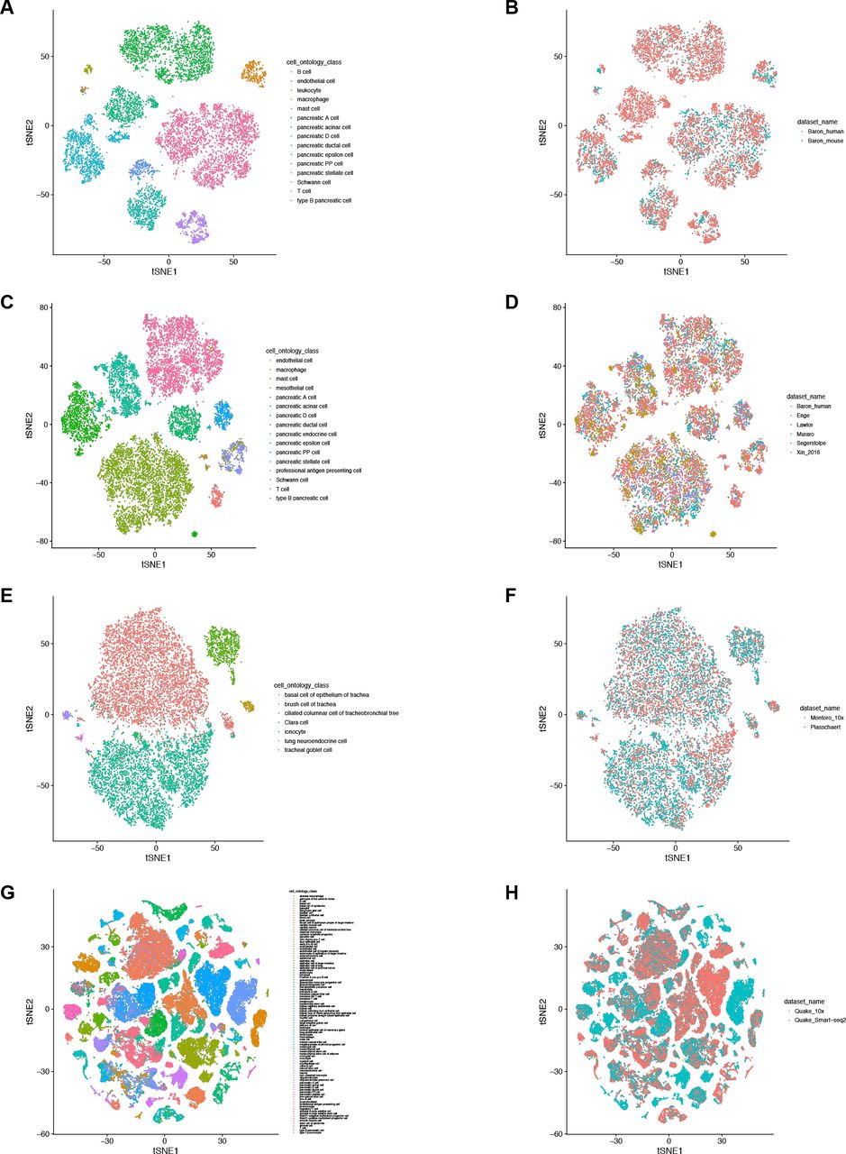
Figures in the left column color cells by their cell types, while figures in the right column color cells by dataset. (A-B) “Baron_human”46 and “Baron_mouse”46; (C-D) “Baron_human”46, “Muraro”43, “Enge”49, “Segerstolpe”50, “Xin_2016”51 and “Lawlor”52; (E-F) “Montoro_10x”14 and “Plasschaert”15; (G-H) “Quake_Smart-seq2”18 and “Quake_10x”18.

(A-C) Latent space learned only with cross-dataset batch correction, colored by (A) donor in “Baron_human”46, (B) donor in “Enge”49, (C) donor in “Muraro”43, respectively. (D-H) Latent space learned with both cross-dataset batch correction and within-dataset batch correction, colored by (D) donor in “Baron_human”46, (E) donor in “Enge”49, (F) donor in “Muraro”43, (G) cell type, (H) dataset, respectively. (I) Standard deviation decreases as number of samples from the posterior increases. (J) Relation between Euclidean distance and posterior distance on “Baron_human”46 data. Orange points represent cell pairs that are of the same cell type (“positive pairs”), while blue points represent cell pairs of different cell types (“negative pairs”). (K) AUROC of different distance metrics in discriminating cell pairs with the same cell type from cell pairs with different cell types. Note that posterior distribution distances for scVI only lead to decrease in performance, possibly due to improper Gaussian assumption in the posterior. (L) Accuracy, Cohen’s κ, specificity and sensitivity all increase as the number of models used for cell querying increases, among which improvement of specificity is most significant.
DR, dimension reduction benchmarking; BC, batch effect correction benchmarking
While the unbiased latent space embedding derived by nonlinear deep neural network effectively removes confounding factors, the network’s random components and nonconvex optimization procedure also lead to serious challenges, especially false positive hits when cells outside reference types are provided as query. Thus, we propose a novel probabilistic cell-to-cell similarity metric in latent space based on posterior distribution of each cell, which we term “normalized projection distance” (NPD). Distance metric ROC analysis (Method) shows that our posterior NPD metric is more accurate and robust than Euclidean distance, which is commonly used in other neural network-based embedding tools (Figure 1D). Additionally, we exploit stability of query-hit distance across multiple models to improve specificity (Methods, Supplementary Figure 4L). An empirical p-value is computed for each query hit as a measure of “confidence”, by comparing posterior distance to the empirical NULL distribution obtained from randomly selected pairs of cells in the queried database.
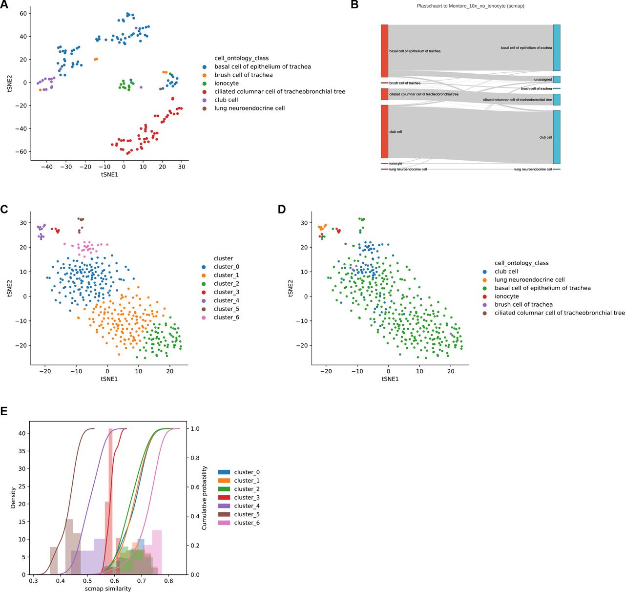
The high specificity of Cell BLAST is especially important for discovering novel cell types. Two recent studies (“Montoro”14 and “Plasschaert”15) independently reported a rare tracheal cell type named pulmonary ionocyte. We artificially removed ionocytes from the “Montoro” dataset, and used it as reference to annotate query cells from the “Plasschaert” dataset. In addition to accurately annotating 95.9% of query cells, Cell BLAST correctly rejects 12 out of 19 “Plasschaert” ionocytes (Figure 1E). Moreover, it highlights the existence of a putative novel cell type as a well-defined cluster with large p-values among all 156 rejected cells, which corresponds to ionocytes (Figure 1F-G, Supplementary Figure 6A, also see Supplementary Figure 5 for more detailed analysis on the remaining 7 cells). In contrary, scmap-cell2 only rejected 7 “Plasschaert” ionocytes despite higher overall rejection number of 401 (i.e. more false negatives, Supplementary Figure 6B-E).

(A) Cell-cell correlation heatmap for several cell types of interest. Cells labeled as “<X>” are reference cells in the “Montoro”14 dataset. Cells labeled as “X->Y” are cells annotated as “X” in the original “Plasschaert”15 dataset but predicted to be “Y”. (B-D) Expression levels of several club cell markers in cell groups of interest. (E-G) Expression levels of several ionocyte markers in cell groups of interest.

(A) t-SNE visualization of Cell BLAST rejected cells, colored by cell type. (B) Sankey plot of scmap prediction. (C, D) t-SNE visualization of scmap rejected cells, colored by unsupervised clustering (C) and cell type (D). (E) scmap similarity distribution in each cluster of scmap rejected cells. The rejected ionocytes do not have the lowest cosine similarity scores to draw enough attention.
We further systematically compared the performance of query-based cell typing with scmap-cell2 and CellFishing.jl4 using four groups of datasets, each including both positive control and negative control queries (first 4 groups in Supplementary Table 2). Of interest, while Cell BLAST shows superior performance than scmap-cell and CellFishing.jl under the default setting (Supplementary Figure 7A-C, 8-10), detailed ROC analysis reveals that performance of scmap-cell could be further improved to a level comparative to Cell BLAST by employing higher thresholds, while ROC and optimal thresholds of CellFishing.jl show large variation across different datasets (Supplementary Figure 7D). Cell BLAST presents the most robust performance with default threshold (p-value < 0.05) across multiple datasets, which largely benefits real-world application. Additionally, we also assessed their scalability using reference data varying from 1,000 to 1,000,000 cells. Both Cell BLAST and CellFishing.jl scale well with increasing reference size, while scmap-cell’s querying time rises dramatically for larger reference dataset with more than 10,000 cells (Supplementary Figure 7E).

(A), sensitivity (B) and Cohen’s κ (C) for different methods under the default setting. (D) ROC curve of cell querying in four different groups of test datasets. Cohen’s κ values in bottom left of each subpanel correspond to the optimal point on ROC curve. Points corresponding to each method’s default cutoff (scmap: cosine distance = 0.5, CellFishing.jl: Hamming distance = 110, Cell BLAST: p-value = 0.05) are marked as triangles. Note that CellFishing.jl does not provide a default cutoff, so we chose Hamming distance of 110 which the closest to balancing sensitivity and specificity, but it’s still far from being stable across different datasets. (E) Querying speed on references of different sizes subsampled from the 1M mouse brain dataset35.

Sankey plots for Cell BLAST in the cell querying benchmark.

Sankey plots for scmap in the cell querying benchmark.

Sankey plots for CellFishing.jl in the cell querying benchmark.
Datasets used in cell query benchmarking.
Moreover, our deep generative model combined with posterior-based latent-space similarity metric enables Cell BLAST to model continuous spectrum of cell states accurately. We demonstrate this using a study profiling mouse hematopoietic progenitor cells (“Tusi”16), in which computationally inferred cell fate distributions are available. For the purpose of evaluation, cell fate distributions inferred by authors are recognized as ground truth. We selected cells from one sequencing run as query and the other as reference to test if we can accurately transfer continuous cell fate between experimental batches (Figure 2A-B). Jensen-Shannon divergence between prediction and ground truth shows that our prediction is again more accurate than scmap (Figure 2C).

(A, B) UMAP visualization of latent space learned on the “Tusi” dataset, colored by sequencing run (A) and cell fate (B). Model is trained solely on cells from run 2 and used to project cells from run 1. Each one of the seven terminal cell fates (E, erythroid; Ba, basophilic or mast; Meg, megakaryocytic; Ly, lymphocytic; D, dendritic; M, monocytic; G, granulocytic neutrophil) are assigned a distinct color. Color of each single cell is then determined by the linear combination of these seven colors in hue space, weighed by cell fate distribution among these terminal fates. (C) Distribution of Jensen-Shannon divergence between predicted cell fate distributions and author provided “ground truth”. (D) UMAP visualization of the “Velten” dataset, colored by Cell BLAST predicted cell fates. (E) Number of organs covered in each species for different single-cell transcriptomics databases, including Single Cell Portal (https://portals.broadinstitute.org/single_cell); Hemberg collection2; SCPortalen19; scRNASeqDB20.
Besides batch effect among multiple reference datasets, bona fide biological similarity could also be confounded by large, undesirable bias between query and reference data. Taking advantage of the dedicated adversarial batch alignment component, we implemented a particular "online tuning" mode to handle such often-neglected confounding factor. Briefly, the combination of reference and query data is used to fine-tune the existing reference-based model, with query-reference batch effect added as an additional component to be removed by adversarial batch alignment (Method). Using this strategy, we successfully transferred cell fate from the above “Tusi” dataset to an independent human hematopoietic progenitor dataset (“Velten”17) (Figure 2D). Expression of known cell lineage markers validates the rationality of transferred cell fates (Supplementary Figure 11A-F). In contrary, scmap-cell incorrectly assigned most cells to monocyte and granulocyte lineages (Supplementary Figure 11G). As another example, we applied “online tuning” to Tabula Muris18 spleen data, which exhibits significant batch effect between 10x and Smart-seq2 processed cells. ROC of Cell BLAST improves significantly after “online tuning”, achieving high specificity, sensitivity and Cohen’s κ at the default cutoff (Supplementary Figure 11H, last group in Supplementary Table 2).

UMAP visualization of the “Velten”17 dataset, colored by expression of lineage markers, including CA1 for erythrocyte lineage (A), GP1BB for megakaryocyte lineage (B), DNTT for B cell lineage, TGFBI for monocyte, dendritic cell lineage (D), CLC for eosinophil, basophil, mast cell lineage (E), MPO for neutrophil lineage (F), and scmap predicted cell fate distribution (G). (H) ROC curve of cell querying in Tabula Muris18 spleen data. Cohen’s κ values in bottom left of each subpanel correspond to the optimal point on ROC curve. Points corresponding to each method’s default cutoff (scmap: cosine distance = 0.5, CellFishing.jl: Hamming distance = 110, Cell BLAST: p-value = 0.05) are marked as triangles.
A comprehensive and well-curated reference database is crucial for practical application of Cell BLAST. Based on public scRNA-seq datasets, we developed a comprehensive Animal Cell Atlas (ACA). With 986,305 cells in total, ACA currently covers 27 distinct organs across 8 species, offering the most comprehensive compendium for diverse species and organs (Figure 2E, Supplementary Figure 12A-B, Supplementary Table 3). To ensure unified and high-resolution cell type description, all records in ACA are collected and annotated with a standard procedure (Method), with 95.4% of datasets manually curated with Cell Ontology, a structured controlled vocabulary for cell types.

(A) Comparison of cell number in different single-cell transcriptomics databases. (B) Composition of different single-cell sequencing platforms in ACA. (C) Home page of the Web interface. (D) Web interface showing results of an example query.
A user-friendly Web server is publicly accessible at http://cblast.gao-lab.org, with all curated datasets and pretrained models available, providing “off-the-shelf” querying service. Of note, we found that our model works well on all ACA datasets with minimal hyperparameter tuning (latent space visualization available on the website). Based on this wealth of resources, users can obtain querying hits and visualize cell type predictions with minimal effort (Supplementary Figure 12C-D). For advanced users, a well-documented python package implementing the Cell BLAST toolkit is also available, which enables model training on custom references and diverse downstream analyses.
By explicitly modeling multi-level batch effect as well as uncertainty in cell-to-cell similarity estimation, Cell BLAST is an accurate and robust querying algorithm for heterogeneous single-cell transcriptome datasets. In combination with a comprehensive, well-annotated database and an easy-to-use Web interface, Cell BLAST provides a one-stop solution for both bench biologists and bioinformaticians
Software availability
The full package of Cell BLAST is available at http://cblast.gao-lab.org
Author contributions
G.G. conceived the study and supervised the research; Z.J.C. and L.W. contributed to the computational framework and data curation; S. L., Z.J.C., and D.C.Y designed, implemented and deployed the website; Z.J.C. and G.G. wrote the manuscript with comments and inputs from all co-authors.
Methods
The deep generative model
The model we used is based on adversarial autoencoder (AAE)21. Denote the gene expression profile of a cell as x ∈ ℝG. The data generative process is modeled by a continuous latent variable z ∈ ℝD (D ≪ G) with Gaussian prior z ∼ N(0, ID), as well as a one-hot latent variable c ∈ {0,1}K, cT c = 1 with categorical prior c ∼ Cat(K), which aims at modeling cell type clusters. A unified latent vector is then determined by l = z + Hc, where H ∈ ℝD×K. A neural network (decoder, denoted by Dec below) maps the cell embedding vector l to two parameters of the negative binomial distribution μ, θ = Dec(l) that models the distribution of expression profile x:

 Where μ and θ are mean and dispersion of the negative binomial distribution. Theoretically, the negative binomial model should be fitted on raw count data8, 13, 22. However, for the purpose of cell querying, datasets have to be normalized to minimize the influence of capture efficiency and sequencing depth. We empirically found that on normalized data, negative binomial still produced better results than alternative distributions like log-normal. To prevent numerical instability caused by normalization breaking the mean-variance relation of negative binomial, we additionally include variance of the dispersion parameter as a regularization term.
Training objectives for the adversarial autoencoder are:


 q(z|x; Enc) and q(c|x; Enc) are “universal approximator posteriors” parameterized by another neural network (encoder, denoted by Enc). Expectations with regard to q(z|x; Enc) and q(c|x; Enc) are approximated by sampling x’ ~ poisson (x) and feeding to the deterministic encoder network. Dz and Dc are discriminator networks for z and c which output the probability that a latent variable sample is from the prior rather than the posterior. Effectively, adversarial training between encoder (Enc) and discriminators (Dn and Dq) drives encoder output to match prior distributions of latent variables p(z) and p(c). λz and λc are hyperparameters that control prior matching strength. The model is much easier and more stable to train compared with canonical GANs because of low dimensionality and simple distribution of z and c.
At convergence, the encoder learns to map data distribution to latent variables that follow their respective prior distributions and the decoder learns to map latent variables from prior distributions back to data distribution. The key element we use for cell querying is vector l on the decoding path, as it defines a unified latent space in which biological similarities are well captured. The model also works if no categorical latent variable is used, in which case l = z directly.
Some architectural designs are learned from scVI8, including logarithm transformation before encoder input, and softmax output scaled by library size when computing μ. Stochastic gradient descent with minibatches is applied to optimize the loss functions. Specifically, we use the “RMSProp” optimization algorithm with no momentum term to ensure stability of adversarial training. The model is implemented using Tensorflow23 python library.
Adversarial batch alignment
As a natural extension to the prior matching adversarial training strategy described in the previous section, also following recent works in domain adaptation24–26, we propose the adversarial batch alignment strategy to align the latent space distribution of different batches. Below, we extend derivation in the original GAN paper27 to show that adversarial batch alignment converges when embedding space distributions of different batches are aligned. In the case of multiple batches, we assume that marginal data distribution can be factorized as below:
 b ∈ {0,1}B, bT b = 1 denotes a one-hot batch indicator, and batch distribution p(b) is categorical:
 Adversarial batch alignment introduces an additional loss:

 ℒbase denotes the loss function in (3). Db is a multi-class batch discriminator network that outputs the probability distribution of batch membership based on embedding vector l. λb is a hyperparameter controlling batch alignment strength. Additionally, the generative distribution is extended to condition on b as well:
 Now, we focus on batch alignment and discard the first ℒbase term and scaling parameter λb. To simplify notation, we fuse data distribution and encoder transformation, and replace the minimization over encoder to minimization over batch embedding distributions:

 Here Dbi (l) denotes the ith dimension of discriminator output, i.e. probability that the discriminator “thinks” a cell is from the ith batch. Db is assumed to have sufficient capacity, which is generally reasonable in the case of neural networks. Global optimum of (12) is reached when Db outputs optimal batch membership distribution at every l:
 Solution to the above maximization is given by:
 Substituting Db∗(l) back into (11), we obtain:
 Thus
Thus  is the global minimum, reached if and only if pi(l) = pj(l), ∀i, j. The minimization of (11) is equivalent to minimizing a form of generalized Jensen-Shannon divergence among multiple batch embedding distributions.
Note that in practice, model training looks for a balance between ℒbase and pure batch alignment. Aligning cells of the same type induces minimal cost in ℒbase, while cells of different types could cause ℒbase to rise dramatically if improperly aligned. During training, gradient from both batch discriminators and decoder provide fine-grain guidance to align different batches, leading to better results than “hand-crafted” alignment strategies like CCA7 and MNN6. Empirically, given proper values for λb, the adversarial approach correctly handles difference in cell type distribution among batches. If multiple levels of batch effect exist, e.g. within-dataset and cross-dataset, we use an independent batch discriminator for each component, providing extra flexibility.
Data preprocessing for benchmarks
Most informative genes were selected using the Seurat7 function “FindVariableGenes”. We set the argument “binning.method” to “equal_frequency” and left other arguments as default. If within dataset batch effect exists, genes are selected independently for each batch and then pooled together. By default, a gene is retained if it is selected in at least 50% of batches. Downstream benchmarks were all performed using this gene set, except for scmap and CellFishing.jl which provide their own gene selection method. GNU parallel28 was used to parallelize and manage jobs throughout the benchmarking and data processing pipeline.
Benchmarking dimension reduction
PCA was performed using the R package irlba29 (v2.3.2). ZIFA12 was downloaded from its Github repository, and hard coded random seeds were removed to reveal actual stability. ZINB-WaVE13 (v1.0.0) was performed using the R package zinbwave. scVI8 (v0.2.3) was downloaded from its Github repository, and minor changes were made to the original code to address PyTorch30 compatibility issues. Our modified versions of ZIFA and scVI are available upon request.
For PCA and ZIFA, data was logarithm transformed after normalization and adding a pseudocount of 1. Hyperparameters of all methods above were left as default. For our model, we used the same set of hyperparameters throughout all benchmarks. λz and λc are both set to 0.001. All neural networks (encoder, decoder and discriminators) use a single layer of 128 hidden units. Learning rate of RMSProp optimizer is set to 0.001, and minibatches of size 128 are used. For comparability, target dimensionality of each method was set to 10. All benchmarked methods were repeated multiple times with different random seeds. Run time was limited to 2 hours, after which the job would be terminated.
Cell type nearest neighbor mean average precision (MAP) was computed with K nearest neighbors of each cell based on low dimensional space Euclidean distance. Denote cell type of a cell as y, and cell type of its ordered nearest neighbors as y1, y2, … yk. Average precision (AP) for that cell is defined as:
 Mean average precision is then given by:
 Note that when K = 1, MAP reduces to nearest neighbor accuracy. We set K to 1% of total cell number throughout all benchmarks.
Benchmarking batch effect correction
We merge multiple datasets according to shared gene names. If datasets to be merged are from different species, Ensembl ortholog31 information is used to map them to ortholog groups. To obtain informative genes in merged datasets, we take the union of informative genes from each dataset, and then intersect the union with the intersection of detected genes from each dataset.
CCA7 and MNN6 alignments were performed using R packages Seurat7 (v2.3.3) and scran32 (v1.6.9) respectively. Hard coded random seeds in Seurat were removed to reveal actual stability. The modified version of Seurat is available upon request. For comparability, we evaluated cell type resolution and batch mixing in a 10-dimensional latent space. For MNN alignment, we set argument “cos.norm.out” to false, and left other arguments as default. PCA was applied to reduce dimensionality to 10 after obtaining the MNN corrected expression matrix. For CCA alignment, we used the first 10 canonical correlation vectors. Run time was limited to 2 hours, after which the job would be terminated. Seurat alignment score was computed exactly as described in the CCA alignment paper7.
Cell querying based on posterior distributions
We evaluate cell-to-cell similarity based on posterior distribution distance. Like in the training phase, we obtain samples from the “universal approximator posterior” by sampling x’ ~ Poission (x) and feeding to the encoder network. In order to obtain robust estimation of distribution distance with a small number of posterior samples, we project posterior samples of two cells onto the line connecting their posterior point estimates in the latent space, and use projected scalar distribution distance to approximate true distribution distance. Wasserstein distance is computed on normalized projections to account for non-uniform density across the embedding space:
 Where
Where
 We term this distance metric normalized projection distance (NPD). By default, 50 samples from the posterior are used to compute NPD, which produces sufficiently accurate results (Supplementary Figure 4I-J). The definition of NPD does not imply an efficient nearest neighbor searching algorithm. To increase speed, we first use Euclidean distance-based nearest neighbor searching, which is highly efficient in the low dimensional latent space, and then compute posterior distances only for these nearest neighbors. Empirical distribution of posterior NPD for a dataset is obtained by computing posterior NPD on randomly selected pairs of cells in the reference dataset. Empirical p-values of query hits are computed by comparing posterior NPD of a query hit to this empirical distribution.
We note that even with the querying strategy described above, querying with single models still occasionally leads to many false positive hits when cell types that the model has not been trained on are provided as query. This is because embeddings of such untrained cell types are mostly random, and they could localize close to reference cells by chance. We reason that embedding randomness of untrained cell types could be utilized to identify and correctly reject them. Practically, we train multiple models with different starting points (as determined by random seeds), and compute query hit significance for each model. A query hit is considered significant only if it is consistently significant across multiple models. To acquire predictions based on significant hits, we use majority voting for discrete variables, e.g. cell type, or averaging for continuous variables, e.g. cell fate distribution.
Distance metric ROC analysis
Our model and scVI8 were fitted on reference datasets and applied to positive and negative control query datasets in the pancreas group of Supplementary Table 2. We then randomly selected 10,000 query-reference cell pairs. A query-reference pair is defined as “positive” if the query cell and reference cell are of the same cell type, and “negative” otherwise. Each benchmarked similarity metric was then computed on all sampled query-reference pairs, and used as predictors for “positive” / “negative” pairs. AUROC values were computed for each benchmarked similarity metric. In addition to Euclidean distance, we also computed posterior distribution distances for scVI (Supplementary Figure 4K). NPD is computed as described in (18), based on samples from the posterior Gaussian. JSD is computed in the original latent space (without projection).
Benchmarking cell querying
For each of the four querying groups, three types of datasets were used, namely reference, positive query and negative query (see Supplementary Table 2 for a detailed list of datasets used in each querying group). For each querying method, cell type predictions for query cells are obtained based on reference hits with a minimal similarity cutoff. Cell ontology annotations in ACA were used as ground truth. Cells with no cell ontology annotations were excluded in the analysis. Predictions are considered correct if and only if it exactly matches the ground truth, i.e. no flexibility based on cell type similarity. This prevents unnecessary bias introduced in the selection of cell type similarity measure. Cells were inversely weighed by size of the corresponding dataset when computing sensitivity, specificity and Cohen’s κ. AUROC was computed using linear interpolation. For scmap2, we varied minimal cosine similarity requirement for nearest neighbors. For Cell BLAST, we varied maximal p-value cutoff used in filtering hits. For CellFishing.jl4, the original implementation does not include a dedicated cell type prediction function, so we used the same strategy as for our own method (majority voting after distance filtering) to acquire final predictions, in which we varied the Hamming distance cutoff used in distance filtering. Lastly, 4 random seeds were tested for each cutoff and each method to reflect stability. Several other cell querying tools (CellAtlasSearch3, scQuery33, scMCA34) were not included in our benchmark because they do not support custom reference datasets.
Benchmarking querying speed
To evaluate scalability of querying methods, we constructed reference data of varying sizes by subsampling from the 1M mouse brain dataset35. For query data, the “Marques” dataset36 was used. For all methods, only querying time was recorded, not including time consumed to build reference indices.
Application to trachea datasets
We first removed cells labeled as “ionocytes” in the “Montoro_10x”14 dataset, and used “FindVariableGenes” from Seurat to select informative genes using the remaining cells. Four models with different starting points were trained on the tampered “Montoro_10x” dataset. We computed posterior distribution distance p-values as mentioned before, and used a cutoff of p-value > 0.1 to reject query cells from the “Plasschaert”15 dataset as potential novel cell types. We clustered rejected cells using spectral clustering (Scikit-learn37 v0.20.1) after applying t-SNE38 to latent space coordinates. Average p-value for a query cell was computed as the geometric mean of p-values across all hits.
Online tuning
When significant batch effect exists between reference and query, we support further aligning query data with reference data in an online-learning manner. All components in the pretrained model, including encoder, decoder, prior discriminators and batch discriminators are retained. The reference-query batch effect is added as an extra component to be removed using adversarial batch alignment. Specifically, a new discriminator dedicated to reference-query batch effect is added, and the decoder is expanded to accept an extra one-hot indicator for reference and query. The expanded model is then fine-tuned using the combination of reference and query data. Two precautions are taken to prevent decrease in specificity caused by over-alignment. Firstly, adversarial alignment loss is constrained to cells that have mutual nearest neighbors6 between reference and query data in each SGD minibatch. Secondly, we penalize the deviation of fine-tuned model weights from original weights.
Application to hematopoietic progenitor datasets
For within-“Tusi”16 query, we trained four models using only cells from sequencing run 2, and cells from sequencing run 1 were used as query cells. PBA inferred cell fate distributions, which are 7-dimensional categorical distributions across 7 terminal cell fates, were used as ground truth. We took the average cell fate distributions of significant querying hits (p-value < 0.05) as predictions for query cells. As for scmap-cell, we filtered nearest neighbors according to default cosine similarity cutoff of 0.5. Jensen-Shannon divergence (JSD) between true and predicted cell fate distribution was computed as below:
 For cross-species querying between “Tusi” and “Velten”17, we mapped both mouse and human genes to ortholog groups. Online tuning with 200 epochs was used to increase sensitivity and accuracy. Latent space visualization was performed with UMAP39, 40.
ACA database construction
We searched Gene Expression Omnibus (GEO)41 using the following search term:
( "expression profiling by high throughput sequencing"[DataSet Type] OR "expression profiling by high throughput sequencing"[Filter] OR "high throughput sequencing"[Platform Technology Type] ) AND "gse"[Entry Type] AND ( "single cell"[Title] OR "single-cell"[Title] ) AND ("2013"[Publication Date]: "3000"[Publication Date]) AND "supplementary"[Filter]Datasets in the Hemberg collection (https://hemberg-lab.github.io/scRNA.seq.datasets/) were merged into this list. Only animal single-cell transcriptomic datasets profiling samples of normal condition were selected. We also manually filtered small scale or low-quality data. Additionally, several other high-quality datasets missing in the previous list were included for comprehensiveness.
The expression matrices and metadata of selected datasets were retrieved from GEO, supplementary files of the publication or by directly contacting the authors. Metadata were further manually curated by adding additional description in the paper to acquire the most detailed information of each cell. We unified raw cell type annotation by Cell Ontology42, a structured controlled vocabulary for cell types. Closest Cell Ontology terms were manually assigned based on Cell Ontology description and context of the study.
Building reference panels for ACA database
Two types of searchable reference panels are built for the ACA database. The first consists of individual datasets with dedicated models trained on each of them, while the second consists of datasets grouped by organ and species, with models trained to align multiple datasets profiling the same species and the same organ.
Data preprocessing follows the same procedure as in previous benchmarks. Both cross-dataset batch effect and within-dataset batch effect are manually examined and removed when necessary. For the first type of reference panels, datasets too small (typically < 1,000 cells sequenced) are excluded because of insufficient training data. These datasets are still included in the second type of panels, where they are trained jointly with other datasets profiling the same organ in the same species. For each reference panel, four models with different starting points are trained. Latent space visualization, self-projection coverage and accuracy on all reference panels are available on our website.
Web interface
For conveniently performing and visualizing Cell BLAST analysis, we built a one-stop web interface. The client-side was made from Vue.js, a the single-page application Javascript framework, and D3.js for cell ontology visualization. We used Koa2, a web framework for Node.js, as the server-side. The Cell BLAST web portal with all accessible curated datasets is deployed on Huawei Cloud.
Acknowledgements
The authors thank Drs. Zemin Zhang, Cheng Li, Letian Tao, Jian Lu and Liping Wei at Peking University for their helpful comments and suggestions during the study. This work was supported by funds from the National Key Research and Development Program (2016YFC0901603), the China 863 Program (2015AA020108), as well as the State Key Laboratory of Protein and Plant Gene Research and the Beijing Advanced Innovation Center for Genomics (ICG) at Peking University. The research of G.G. was supported in part by the National Program for Support of Top-notch Young Professionals. Part of the analysis was performed on the Computing Platform of the Center for Life Sciences of Peking University, and supported by the High-performance Computing Platform of Peking University.
Main text references
Supplementary references


